Correct Stability Condition and Fundamental Performance Analysis of the α-β-γ-δ Filter


Department of Intelligent Systems Design Engineering, Graduate School of Engineering, Toyama Prefectural University, Imizu, Toyama 939-0398, Japan
*
Author to whom correspondence should be addressed.
Appl. Sci. 2018, 8(12), 2523; https://0-doi-org.brum.beds.ac.uk/10.3390/app8122523
Submission received: 26 October 2018
/
Revised: 29 November 2018
/
Accepted: 5 December 2018
/
Published: 6 December 2018
Abstract
:Featured Application
Moving object tracking in robots and intelligent vehicles
Abstract
This paper theoretically analyzes the fundamental performance of a fourth-order steady-state moving object tracking filter, called an --- filter. The --- filter considers estimations of jerk (time-derivative of acceleration) in the motion of targets. First, regarding the stability conditions of the --- filter, we prove that there are unstable cases even when the conventionally derived stability conditions are satisfied, and then we derive the correct stability conditions. Next, we analytically derive performance indices that indicate the steady-state errors for targets with typical motions. Based on the derived indices, the optimal performance of the --- filter is theoretically analyzed and compared with that of the traditional second- and third-order steady-state tracking filters, i.e., - and -- filters. Numerical analyses and simulations are used to verify the advantages and disadvantages of the --- filter over the above-mentioned filters. The practicality of the use of jerk for the tracking filtering problem is revealed in this paper.
1. Introduction
In monitoring systems for aircraft, robots, and intelligent cars using remote sensors such as radar and cameras, the accurate tracking of moving objects is essential. For such applications, Kalman filter- [1,2,3,4] and Bayesian filter-based trackers [5] are commonly used to track the position, velocity, and acceleration of the targets. However, in recent years, the importance of jerk, which is the derivative of acceleration with respect to time, has been realized to address tracking problems [4,6,7]. In [4,6], it was proved that the use of a high-dimensional parameter such as jerk can improve the performance of the tracking filters for highly maneuvering targets. Thus, the consideration of jerk in tracking filters is promising. However, commonly used and well-analyzed conventional tracking filters do not consider tracking jerk. A steady-state second-order Kalman filter, known as an - filter [8,9,10], tracks position and velocity only, and a steady-state third-order tracking filter, known as an -- filter [6,11,12,13], tracks these in addition to acceleration.
To estimate and use the jerk in tracking filters, Wu et al. [14] proposed a steady-state fourth-order Kalman filter considering jerk tracking, which is called an --- filter, and they analyzed its performance by determining its transfer functions and stability conditions [14]. However, their correctness has not been proved and validated. Furthermore, they also proposed a simulation-based optimal design and performance analysis of the --- filter using the Taguchi method, evolution-programming, and genetic- algorithm [14,15,16], but the theoretical performance of the filter has not been analyzed. Furthermore, these studies have investigated some limited setting of the filter parameters (filter gains). Jeong et al. also performed optimal design using a fading memory filter algorithm for the --- filter [17]. However, its optimal quality and effectiveness in general situations are not guaranteed. Thus, the performance of the --- filter has not been analyzed and validated theoretically, and its advantages over the traditional - and -- filters are unknown. In other words, the selection criteria for the above filters for practical use have not been established.
In this paper, we theoretically analyze the steady-state performance of the --- filter by deriving its closed-form performance indices. First, we show an example in which the filter is unstable even when the stability conditions derived by Wu et al. [14] are satisfied, and then, we derive the correct conditions to ensure convergence of the steady state for the --- filter. Then, the steady-state errors for targets moving with constant jerk or snap (time-derivative of the jerk) are derived in closed form as the analytical performance indices of the --- filter. Finally, to investigate the advantages and disadvantages of the --- filter, the performance with optimal gains that are obtained with the derived indices are compared with those of traditional - and -- filters using theoretical analyses and numerical simulations.
Table 1 lists the main symbols used in this paper.
2. The --- Filter
2.1. Problem Definition
We investigate the position prediction performance using a filter called the --- filter [14]. For simplicity, one-dimensional tracking along the x-axis is considered.
The tracking process of the --- filter is as follows. Similar to other tracking filters, the --- filter invokes an iterative prediction and smoothing process to estimate the state of the target. The state of the target includes the position, velocity, acceleration, and jerk (fourth-order tracking). The prediction process is conducted under the assumption that the target’s jerk is constant during a sampling interval, which is expressed as:
where is the predicted position at time , T is the sampling interval, is the smoothed target position, is the predicted velocity, is the smoothed velocity, is the predicted acceleration, is the smoothed acceleration, is the predicted jerk, and is the smoothed jerk. The smoothing process is defined as:
where is the measured position, and , , , and are dimensionless filter gains. In the steady state, the filter gains are converged to a fixed value. Thus, the --- filter uses fixed gains. The definition of the smoothing process in this paper is slightly different from that in Wu’s study [14,15,16]. Their study sets gains corresponding to the acceleration and jerk as and , respectively. However, this study uses the above definition to improve the mathematical generality. Equations (1)–(8) are the definitions of the --- filter.
As indicated in the description of the filtering process above, the input of the filter is . Although eight outputs can be considered (predicted target position , velocity , acceleration , and jerk , and smoothed target position , velocity , acceleration , and jerk ), this paper focuses on the accuracy of because many applications of the tracking filters are focused on the prediction of the position of the target. This study assumes that the error in is due to white Gaussian noise, and the variance of the position measurement error is known.
2.2. Fundamental Properties Obtained in Conventional Studies
2.2.1. Transfer Function and Stability Conditions
In [14], Wu et al. derived the transfer function and Bounded Input-Bounded Output (BIBO) stability conditions of the --- filter using the z-transform of definitions (1)–(8). Considering the difference in the definition of the smoothing process described above, the transfer function for the input and output is expressed as
where and are the z-transforms of and , respectively, and
is a characteristic polynomial of the --- filter.
2.2.2. Relationship to Kalman Filter
The --- filter is equivalent to a steady-state Kalman filter with a constant-jerk model [14,15], which is similar to the well-known conventional - and -- filters [8,12]. The equations for the Kalman filter are:
where x is a state vector, forecasts and estimates are denoted by tildes and hats, respectively, superscript ”T” and ”” denote transpositions and inversions, z is a measurement vector, F is the transition matrix, is the error covariance matrix at time , Q is the covariance matrix for the process noise, is the optimal gain (Kalman gain) at time , and B is the covariance matrix for the measurement noise. The --- filter is obtained by substituting the following into (15) and (19): Vectors , , , and matrices:
By assuming the steady state with , the gains in (22) become constant and the --- filter of definitions (1)–(8) is obtained. Thus, the investigation of the properties of the --- filter is equivalent to that of the steady-state properties of the fourth-order Kalman filter tracker.
2.2.3. Relationship to the - and -- Filters
As indicated above, the --- filter is a fourth-order filter. Traditionally, the steady-state second- and third-order tracking filters are well known as - and -- filters, respectively. These filters are popularly used because of their simplicity, utility in real-time applications, and usefulness in the design of complicated tracking systems.
The - filter is a steady-state second-order Kalman filter using the constant-velocity model that tracks the position and velocity of moving objects. Its filtering process is as follows [8]:
Please note that the smoothing processes of (26) and (27) are the same as those of (5) and (6).
Similarly, the -- filter is a steady-state third-order Kalman filter using the constant acceleration model; thus, it tracks the position, velocity, and acceleration of moving objects. Its filtering process is as follows [11]:
Please note that the smoothing processes of (31)–(33) are the same as those of (5)–(7). That is, the --- filter is an extension of these filters.
2.2.4. Performance Analysis Method
The performance of the --- filter is investigated using a simulation-based approach. The difference in the tracking accuracy between this and the -- filters is determined via simulations and adaptive gain calculations [14,15,16,17]. However, a theoretical analysis of the performance is not conducted and the appropriateness of the gain setting is not guaranteed. In the simulation-based gain settings presented in [15,16], the considered gain values are limited (e.g., is set only 0.1, 0.7, 1.3, or 1.9). Thus, it seems that the performance and filter stability are only considered for these limited gain settings. Furthermore, the simulations only consider some situations, and the general advantages and disadvantages of the --- filter are not clarified.
In contrast, two theoretical performance indices are used for the performance analysis and optimal gain setting of the conventional - and the -- filters [8,13]. One is the tracking performance index, which evaluates the performance for the prediction of maneuvering motions. The tracking performance is defined by the steady-state bias error as follows:
where is the true motion of the target moving with a constant one-order-higher motion parameter compared with that in the filter’s motion model. For example, is the constant accelerating motion for the - filter because this assumes the constant-velocity model for the prediction process. Similarly, is the constant-jerk motion for the -- filter. The other is the smoothing performance index, which evaluates the performance of noise reduction in the filtering process. The smoothing performance is defined by the steady-state error variance as follows:
where denotes the mean with respect to k and is the true motion of the target moving with the same motion as that in the prediction model. Thus, is the constant-velocity motion for the - filter, and is the constant acceleration motion for the -- filter.
These performance indices of the - and the -- filter have been reported in many studies [8,9,11,12,13] (also see Table 2 of this paper), and they have effectively been used for performance analysis and gain design. This is because that these indices are expressed in closed form and empirical simulation-based performance analysis and filter gain design are not required. However, these indices of the --- filter have not been derived and hence, their theoretical performance has not been analyzed.
In summary, the fundamental properties of the --- filter, the stability conditions, and the tracking/smoothing performance have not been validated. Thus, in the rest of this paper, these are derived and the theoretical performance of the --- filter based on the derived performance indices is determined to clarify the optimal performance and the difference in the performance between this filter and the conventional - and the -- filters.
3. Derivation of Correct Stability Condition
This section presents a reconsideration of the stability conditions of the --- filter. As described in the previous section, the conventionally obtained stability conditions are expressed as (11)–(14). However, there are some cases where the filter outputs diverge even when the conventional stability conditions (11)–(14) are satisfied. An example of this type of case is shown in Appendix A. Hence, the correct BIBO stability conditions can be derived from the characteristic polynomial of (10) using Jury’s stability test [18]. Based on Jury’s table presented in Appendix B, the stability conditions of the --- filter are as follows:
where
Please note that these derived conditions comply with the conventional stability conditions.
4. Steady-State Performance Index and Optimal Gains
We derive the indices for the tracking performance (steady-state bias error) and the smoothing performance (steady-state variance of random errors) of the --- filter. Furthermore, the optimal gains are calculated using the derived indices to analytically investigate the optimal performance of the --- filter.
4.1. Derivation of Tracking Performance Index
The tracking performance index is derived using (34). During tracking with the --- filter, a steady-state bias error occurs for the target moving with a constant snap (time-derivative of jerk) because of the difference between the motion of the model (constant-jerk model) and the motion of the target. Thus, the tracking performance, that is, the steady-state predicted error, is calculated by (34) assuming the true target position = ( denotes a constant snap) and measurement errors are not considered, as
Equation (42) is calculated using the transfer function of (9) and the final value theorem given in Appendix C. The derivation result is
The important aspect here is that the tracking performance is determined by the gain , and it does not depend on other gains.
4.2. Derivation of Smoothing Performance Index
The smoothing performance index is derived using (35). We assume that contains noise with variance and the target moves with a constant jerk because the --- filter uses the constant-jerk motion model, as indicated in (4). Thus, the true motion assumed in (35) is
where , , and are the true velocity, acceleration, and jerk of the target, respectively, used for deriving the smoothing performance index. By calculating (35) using definitions (1)–(8) and (44), the smoothing performance index of the --- filter is derived as:
where
The derivation of is given in Appendix D.
4.3. Comparison of Performance Indices with Those of Conventional Filters
Table 2 summarizes the derived performance indices of the --- filter and those of the conventional - and -- filters. As seen, the tracking performance of the n-th-order filter depends on the inverse of the gain of the n-th motion parameter. This indicates that the degree of the bias error due to the maneuvering motion of the target increases when a small gain is set for the highest-order motion parameter (velocity of the - filter, acceleration of the -- filter, and jerk of the --- filter).
4.4. Calculation of Optimal Smoothing Performance
To investigate the optimal performance of the --- filter, the optimal gains are set to achieve lower derived indices. For this purpose, we use the minimum-variance (MV) filter criterion [9]. The lower the tracking/smoothing performance indices, the better the tracking filter. However, there is a trade-off between them [8]. Thus, to appropriately consider this trade-off, the MV filter criterion is used to calculate the gains that minimize the smoothing performance index under the condition that the tracking performance index is constant. That is, the optimal gains are determined by solving the following minimization problem using the tracking performance (43), the smoothing performance (45)–(47), and the derived stability conditions:
The optimal , , and are obtained for each by solving this problem, and the optimal (minimal) smoothing performance index is calculated by substituting these solutions for the smoothing performance (45)–(47). The above problem is solved using the simple gradient descent method. By solving the above problem, the optimal quality of the filter is theoretically guaranteed, in contrast to the conventional simulation-based gain design methods [14,15,16].
5. Theoretical Analysis Using Performance Indices
We theoretically analyze and compare the performance of the -, --, and --- filters using the optimal smoothing performance index calculated in the above process. We analyze the relationship between the optimal smoothing performance index and the gain that determines the tracking performance for each filter ( of the - filter, of the -- filter, and of the --- filter as indicated in Table 2). Since the tracking performance index indicates the bias error of each filter, the setting values for these gains correspond to identical settings of bias errors for all filters when the other parameters are normalized. Thus, the smoothing performances for random errors of all filters are impartially compared under the same bias error. We assume that T and are normalized to 1.
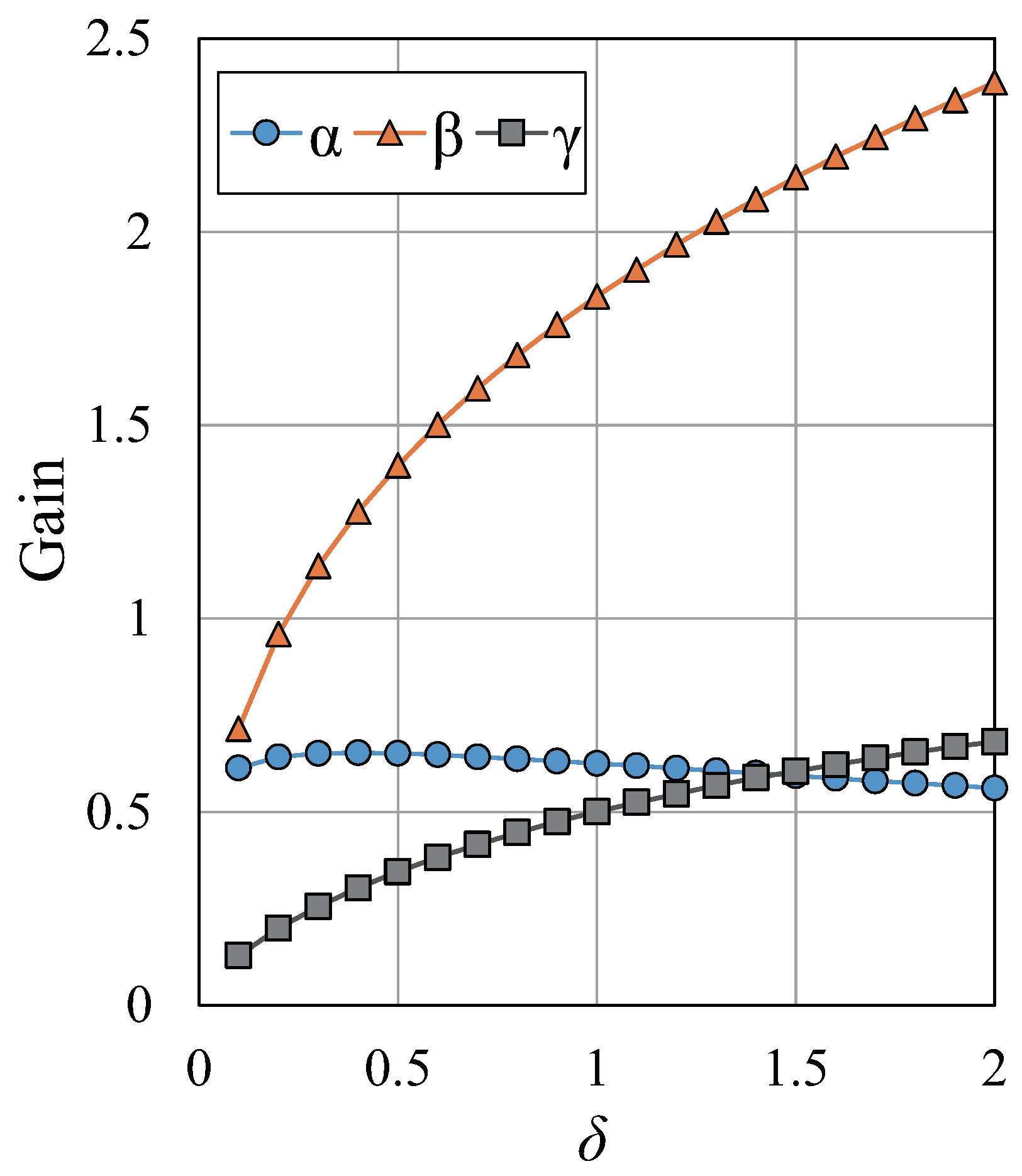
First, we clarify the optimal gains of the --- filter by solving the minimization problem (50). Figure 1 shows the optimal , , and for each of the --- filter. As shown, the optimal and increase with increasing . This is because a large is suitable for tracking high-maneuvering targets, as indicated in the tracking performance index of (43), and and also increase to track the velocity and acceleration with a relatively large variation. In contrast, the optimal does not have a large variation to maintain the smoothing function of the tracking filter.
Then, the optimal smoothing performance index is calculated using these gains. Figure 2 shows the results of the calculations. This figure also plots the optimal of the - and -- filters for comparison. As shown in the figure, when the tracking performance improves (the fixed gain for each filter becomes large), the smoothing performance of the --- filter decreases compared with that of the conventional filters. This means that although the --- filter can track complicated motion including the jerk by setting large gains, the errors caused by the measurements are not sufficiently suppressed compared with those in the conventional filters. Moreover, the smoothing performance deterioration of the --- filter compared with that of the -- filter is larger than that of the -- filter compared with that of the - filter. These results show that there will be a further decrease in the smoothing performance with the increasing order of the tracking filter. That is, it is not effective to increase the order of the tracker when the target motion is relatively simple such as targets moving with nearly constant velocity and acceleration. Figure 2 demonstrates the quantitative difference among the filters’ smoothing performance against related bias errors.
6. Numerical Simulation
This section provides examples of the numerical simulation used to validate the analysis results. We consider two scenarios:
- Simple-maneuvering target assuming constant acceleration or jerk motion.
- High-maneuvering target assuming complicated motion.
In all simulations, the measurement position is calculated by adding white Gaussian noise, the variance of which is , to the true position of the target . We evaluate the RMS predicted error of a Monte Carlo simulation run 300 times that is defined as
where is the predicted position in the m-th Monte Carlo simulation.
6.1. Tracking of Simple-Maneuvering Target
First, a simple-maneuvering target moving with constant acceleration or jerk is considered to validate the above theoretical analysis. For the target with constant acceleration, neither the predicted positions obtained by the -- filter nor the --- filter include bias error due to target motion, because they consider constant acceleration or jerk. Thus, the consideration of constant acceleration motion indicates the difference of the reduction in performance of random errors between these filters. In contrast, the - includes bias error due to acceleration of the target. Thus, the simulation assuming constant acceleration compares the errors of the - filter that consist of both random and bias errors against those of the -- filter and the --- filter, which are affected by random errors only. On the other hand, for the target with constant jerk, the -- filter also has bias errors due to the difference between the motion model and the motion of the target. Thus, the simulation assuming constant jerk compares the errors of the -- filter that consist of both random and bias errors against those of the --- filter.
Values of T = 1 s and = 25 m are set. In terms of the gain settings, we set identical values for the gains that determine the tracking performance index (i.e., we set the same value for of the --- filter, of the -- filter, and of the - filter). Cases of both low and high gain are investigated. In the former, although the smoothing function of filters becomes relatively large, the bias error due to the complicated motion of the target also increases. In contrast, this kind of bias error is suppressed in the latter case. However, the smoothing performance for the random errors decreases. The gain settings in the two cases are as follows:
- Low gain case: ( = 0.266, = 0.1) for the - filter, ( = 0.738, = 0.165, = 0.1) for the -- filter, and ( = 0.613, = 0.715, = 0.128, = 0.1) for the --- filter.
- High gain case: ( = 0.475, = 1.5) for the - filter, ( = 1.354, = 0.560, = 1.5) for the -- filter, and ( = 0.593, = 2.14, = 0.605, = 1.5) for the --- filter.
6.1.1. Scenario 1: Constant Acceleration Target
In this scenario, the true motion of a target is set as
Figure 3a shows the simulation results for the low gain case (). The steady-state errors of the -, --, and --- filters were 320 m, 5.48 m, and 8.27 m, respectively. Because the target motion includes relatively high acceleration, the - filter cannot track the target with sufficient accuracy. In contrast, the other two filters track this target with a higher accuracy. The best performance is achieved with the -- filter because a constant acceleration model is assumed for the prediction process. Although the --- filter can also track accelerating motion, its larger smoothing performance index compared with that of the -- filter demonstrated in Figure 2 leads to a larger error. In addition, the variance of the errors in the - filter is small compared with that of other filters. This is because the - filter largely suppresses random errors compared with other filters, as indicated in the analysis results.
Figure 3b shows the simulation results for the high gain case (). The steady-state errors of the -, --, and --- filters were 24.4 m, 17.2 m, and 24.5 m, respectively. The performance of the --- is worse in this case. This is because of the larger deterioration in the smoothing performance, as demonstrated in Figure 2. In addition, although the accuracy of the - filter decreases due to the high gain setting, it is still quite high. Thus, in this case, the -- filter achieves a better accuracy.
6.1.2. Scenario 2: Constant-Jerk Target
In this scenario, the true motion of a target is set as
Figure 4a shows the simulation results for the low gain case (). The steady-state errors of the -- and --- filters were 960.4 m and 8.29 m, respectively. Because the -- filter assumes a constant acceleration model, the tracking of the target moving with jerk includes large bias errors. Furthermore, the - filter theoretically diverges for tracking with constant jerk. In contrast, the --- filter can accurately track a target moving with jerk even when the gain is low.
Figure 4b shows the simulation results for the high gain case (). The steady-state errors of the -- and --- filters were 66.2 m, and 24.5 m, respectively. Owing to the relatively high gain setting, the -- filter can achieve a higher accuracy to some extent. However, the --- filter also achieves a better accuracy. These results clearly demonstrate the advantage and disadvantage of the --- filter implied by the theoretical analysis.
6.2. Tracking of High-Maneuvering Target
Finally, the performance of the three filters is compared for high-maneuvering target tracking. We can predict that the --- filter achieves better performance for relatively complicated motion, including large jerk, compared with the - and -- filters. The aim of this simulation is to confirm the effectiveness of the --- filter when the target has high-maneuvering motion. The measurement position is obtained by adding white Gaussian noise with to the true position . The true position is set as
Figure 5 shows the and corresponding true snap of the target. Based on this motion, we set and calculate the optimal parameters. We evaluate the RMS prediction error using (51). To fairly compare the performance, the bias errors (tracking performance indices) that correspond to the maximum motion parameters of the targets are set to the same value for all the filters. We assume two cases of gain settings: a low gain case ( of the --- filter is 0.01, of the -- filter is 0.08, and of the - filter is 0.7) and a high gain case ( of the --- filter is 0.05, of the -- filter is 0.4, and of the - filter is 3.5).
Figure 6a shows the simulation results for the low gain case. When the gains are low, the smoothing effect of the measurement noises increases. Thus, for all filters, when the parameters of the target motion (velocity, acceleration, jerk, snap, etc.) are relatively small, i.e., approximately , the RMS errors converge. In this case, the tracking accuracy of the - filter is larger than that of the other two filters. This result is consistent with that of the theoretical analysis shown in Figure 2. In contrast, for , the RMS errors vary because of the bias errors caused by the complicated motion. When the snap of the target increases, the RMS error of the --- filter is the smallest. However, when this is not the case, the RMS error of the --- filter increases due to the poor smoothing performance.
Figure 6b shows the results for the high gain case. In this case, all the filters converge during the observation period. This is because the relatively large gain makes it possible to track complicated large motions. However, due to the poor tracking performance for the maneuvering motion, the - and -- filters generate larger RMS errors compared with those in Figure 6a. In contrast, this type of deterioration in the tracking accuracy for the --- filter is small owing to its better tracking performance for complicated motions including large jerk and snap.
7. Conclusions
This paper clarifies the stability condition and theoretical performance of the steady-state fourth-order tracking filter, i.e., the --- filter that tracks the velocity, acceleration, and jerk of moving objects. First, the stability conditions of the filter were derived using the Jury stability criterion. Then, the tracking and smoothing performance indices of the --- filter were analytically derived in the closed form. The optimal smoothing performance of the --- filter was analyzed and compared with that of the conventional - and -- filters. The results indicated a relatively large deterioration in the smoothing performance of the --- filter. This indicated that although it can track more complicated motion than the conventional low-order filter, its tracking accuracy is poor for tracking simple motion such as constant-velocity motion. However, the numerical simulation assuming a maneuvering target showed the --- filter is ideal for tracking complicated motion including large jerk and snap.
Because the --- filter is one-dimensional tracking filter, this paper assumed the tracking problem along x-axis only. Extensions to our performance analysis to 2- and 3-dimensional problems are important future tasks. Furthermore, an experimental study to validate the filters in real-world environments is the focus of our future work.
Author Contributions
K.S. designed this research; T.S. derived and calculated main results of this paper including the numerical analyses and simulations; T.S. and K.S. wrote the paper; K.S. approved the final manuscript.
Funding
This research was supported by the JSPSKAKENHI Grant No. 16K16093.
Conflicts of Interest
The authors declare no conflict of interest.
Appendix A. An Example of Unstable Case that Satisfy the Conventional Stability Conditions
When we set , , , and for the --- filter, these gains satisfy the conventional stability conditions (11)–(14). We substitute these gains in the characteristic polynomial as:
Thus, the poles of this polynomial are:
Thus, we have , which indicates that the --- filter with the above gain setting is unstable. With the above setting, of the --- filter actually diverged in a numerical simulation assuming a target moving with constant velocity and . We have confirmed that the conventional stability conditions are satisfied in most cases. However, this example indicates that there are some cases for which the filter becomes unstable even when the conventional stability conditions are met.
Appendix B. Jury’s Stability Test for α-β-γ-δ Filter
The necessary and sufficient conditions for the stability of the --- filter are derived using the Jury’s test [18]. The Jury’s table of the characteristic polynomial is shown in Table A1, where:
Using this table, the stability conditions are obtained for the following conditions:
By solving and simplifying (A6)–(A10), we obtain the stability conditions (36)–(39).

Table A1.
Jury’s table for .
| Row | |||||
|---|---|---|---|---|---|
| a | |||||
| b | |||||
| c | |||||
Appendix C. Derivation of the Tracking Performance Index
The transfer function of the --- filter is expressed as (9) and (10):
Using this transfer function, we calculate in the z-domain to derive the tracking performance index (42). The z-transform of the first term is
where Z[] denotes the z-transform. The predicted error in the z-domain is defined as
Here, to calculate the steady-state bias error (mean error), we assume that the mean error in becomes zero because of the white Gaussian noise. Thus, is satisfied. By substituting (A13) and (A11) into (A14), we obtain
By applying the final value theorem to (A15), the tracking performance (43) is derived as follows:
Appendix D. Derivation of the Smoothing Performance Index
The of the --- filter is directly derived from definitions (1)–(8). is the true motion of the constant-jerk target expressed as
Using the definition of prediction process (1) and (A17), the predicted error is calculated as
This indicates that it is necessary to derive the error variances/covariances of the smoothed parameters to obtain . Based on the smoothing process (5)–(8), the quantities , , , and can be expressed as:
By substituting the true motion of the constant-jerk target (A17) into these equations, we obtain:
Using these, and substituting the definition of prediction process (1)–(4) into the definition of smoothing process (5)–(8), we obtain the errors in these smoothed parameters as follows:
From the definition of prediction process (1)–(4) and the true motion of the constant-jerk target (A17), and by defining , , , and , we have:
Thus, the variances of the errors in the smoothed positions can be calculated using (A31) as
Because we have assumed , the variances and covariances of the errors do not depend on k. Consequently, we can define the variances and covariances of the smoothing process as
In addition, the following relations are satisfied because the smoothed parameters are a linear combination of the measured parameters:
By substituting (A36) into (A35) and simplifying the expression using the position measurement error , we have
In a similar manner, we calculate the following variances and covariances of the errors for all parameters: , , and . The results of the calculations are:
By substituting the solutions of the linear system involving (A38)–(A47) into the predicted error (A18) and by using the definitions of the variances and covariances of the smoothing process (A36), we obtain the smoothing performance index (45).
References
- Liu, Z.; Fu, X.; Gao, X. Co-Optimization of Communication and Sensing for Multiple Unmanned Aerial Vehicles in Cooperative Target Tracking. Appl. Sci. 2018, 8, 899. [Google Scholar] [CrossRef]
- Nguyen, N.H.; Dogancay, K. Instrumental Variable Based Kalman Filter Algorithm for Three-Dimensional AOA Target Tracking. IEEE Sign. Process. Lett. 2018, 25, 1605–1609. [Google Scholar] [CrossRef]
- Fan, Y.; Lu, F.; Zhu, W.; Bai, G.; Yan, L. A Hybrid Model Algorithm for Hypersonic Glide Vehicle Maneuver Tracking Based on the Aerodynamic Model. Appl. Sci. 2017, 7, 159. [Google Scholar] [CrossRef]
- Zhang, H.; Xie, J.; Ge, J.; Lu, W.; Zong, B. Adaptive Strong Tracking Square-Root Cubature Kalman Filter for Maneuvering Aircraft Tracking. IEEE Access 2018, 6, 10052–10061. [Google Scholar] [CrossRef]
- Li, T.; Corchado, J.M.; Bajo, J.; Sun, S.; Paz, J.F.D. Effectiveness of Bayesian filters: An information fusion perspective. Inf. Sci. 2016, 329, 670–689. [Google Scholar] [CrossRef]
- Saho, K.; Takahashi, Y.; Masugi, M. Moving object tracker using sensor fusion of ultrasonic range finder and accelerometer. J. Int. Counc. Electric. Eng. 2017, 7, 34–40. [Google Scholar] [CrossRef]
- Yazdani, M.; Gamble, G.; Henderson, G.; Nielsen, R.H. A simple control policy for achieving minimum jerk trajectories. Neural Netw. 2012, 27, 74–80. [Google Scholar] [CrossRef] [PubMed]
- Ekstrand, B. Some aspects on filter design for target tracking. J. Control Sci. Eng. 2012, 2012, 10. [Google Scholar] [CrossRef]
- Kosuge, Y.; Ito, M. Evaluating an α-β filter in terms of increasing a track update-sampling rate and improving measurement accuracy. Electron. Commun. Jpn. Part I Commun. 2003, 86, 10–20. [Google Scholar] [CrossRef]
- Matsunami, I.; Nakamura, R.; Kajiwara, A. Target State Estimation Using RCS Characteristics for 26GHz Short-Range Vehicular Radar. In Proceedings of the 2013 International Conference on Radar, Adelaide, Australia, 9–12 September 2013; pp. 304–308. [Google Scholar]
- Tenne, D.; Singh, T. Characterizing performance of α-β-γ filters. IEEE Trans. Aerosp. Electron. Syst. 2002, 38, 1072–1087. [Google Scholar] [CrossRef]
- Kosuge, Y.; Ito, M. A necessary and sufficient condition for the stability of an α-β-γ filter. In Proceedings of the 40th SICE Annual Conference, Nagoya, Japan, 25–27 July 2001; pp. 7–12. [Google Scholar]
- Saho, K.; Masugi, M. Performance analysis of α-β-γ filters using position and velocity measurements. EURASIP J. Adv. Sign. Process. 2015, 2015, 35. [Google Scholar] [CrossRef]
- Wu, C.M.; Lin, P.P.; Han, Z.Y.; Li, S.R. Simulation-based Optimal Design of α-β-γ-δ Filter. Int. J. Autom. Comput. 2010, 7, 247–253. [Google Scholar] [CrossRef]
- Wu, C.M. Adaptive parameters for tracking filters innovation system. Adv. Mech. Eng. 2016, 8. [Google Scholar] [CrossRef]
- Yu, T.Y.; Wu, C.M. Application of Adaptive α-β-γ and α-β-γ-δ Filter to Tracking Systems. Sens. Mater. 2017, 29, 419–427. [Google Scholar]
- Jeong, T.G.; Pan, B.F.; Njonjo, A.W. A Study of Optimization of α-β-γ-η Filter for Tracking a High Dynamic Target. J. Korean Navig. Port Res. 2017, 11, 297–302. [Google Scholar] [CrossRef]
- Jury, E.I. Theory and Application of the z-Transform Method; John Wiley and Sons: New York, NY, USA, 1964. [Google Scholar]
Figure 1.
Optimal gains of --- filter.

Figure 2.
Relationship between tracking and smoothing performance indices of filters.

Figure 3.
Simulation results for target with constant acceleration. (a) Low gain case; (b) High gain case.
Figure 3.
Simulation results for target with constant acceleration. (a) Low gain case; (b) High gain case.

Figure 4.
Simulation results for target with constant jerk. (a) Low gain case; (b) High gain case.

Figure 5.
True target motion for simulations of high-maneuvering target. (a) True position; (b) True snap.
Figure 5.
True target motion for simulations of high-maneuvering target. (a) True position; (b) True snap.

Figure 6.
Simulation results for high-maneuvering target. (a) Low gain case; (b) High gain case.

Table 1.
List of main symbols.
| Variables | Description | Unit |
|---|---|---|
| T | Sampling interval | [s] |
| k | Discrete sampling index | Dimensionless |
| Parameter at index k | ||
| Predicted position | [m] | |
| Predicted velocity | [m/s] | |
| Predicted acceleration | [m/s] | |
| Predicted jerk | [m/s] | |
| Smoothed (estimated) position | [m] | |
| Smoothed (estimated) velocity | [m/s] | |
| Smoothed (estimated) acceleration | [m/s] | |
| Smoothed (estimated) jerk | [m/s] | |
| Observed (measured) position | [m] | |
| Filter gain for | Dimensionless | |
| Filter gain for | Dimensionless | |
| Filter gain for | Dimensionless | |
| Filter gain for | Dimensionless | |
| Error variance of | [m] | |
| E | Mean with respect to k | |
| Smoothing performance index | [m] | |
| Tracking performance index | [m] | |
| Snap assumed in the derivation of | [m/s] | |
| RMS prediction error of Monte Carlo simulations | [m] |
Table 2.
Performance indices of -, --, and --- filters. The tracking performance indices are normalized by the motion parameter and sampling interval. The smoothing performance indices are normalized by .
Table 2.
Performance indices of -, --, and --- filters. The tracking performance indices are normalized by the motion parameter and sampling interval. The smoothing performance indices are normalized by .
| Tracking Performance (Normalized) | Smoothing Performance (Normalized) | |
|---|---|---|
| - filter | [8] | [8] |
| -- filter | [13] | [13] |
| --- filter | (Equation (43)) | Equations (45)–(47) |
© 2018 by the authors. Licensee MDPI, Basel, Switzerland. This article is an open access article distributed under the terms and conditions of the Creative Commons Attribution (CC BY) license (http://creativecommons.org/licenses/by/4.0/).
Share and Cite
MDPI and ACS Style
Shibata, T.; Saho, K. Correct Stability Condition and Fundamental Performance Analysis of the α-β-γ-δ Filter. Appl. Sci. 2018, 8, 2523. https://0-doi-org.brum.beds.ac.uk/10.3390/app8122523
AMA Style
Shibata T, Saho K. Correct Stability Condition and Fundamental Performance Analysis of the α-β-γ-δ Filter. Applied Sciences. 2018; 8(12):2523. https://0-doi-org.brum.beds.ac.uk/10.3390/app8122523
Chicago/Turabian StyleShibata, Takanori, and Kenshi Saho. 2018. "Correct Stability Condition and Fundamental Performance Analysis of the α-β-γ-δ Filter" Applied Sciences 8, no. 12: 2523. https://0-doi-org.brum.beds.ac.uk/10.3390/app8122523
Note that from the first issue of 2016, this journal uses article numbers instead of page numbers. See further details here.