Pneumatic Rotary Actuator Position Servo System Based on ADE-PD Control

Abstract

In order to accurately control the rotation position of a pneumatic rotary actuator, the flow state of the gas and the motion state of the pneumatic rotary actuator in the pneumatic rotary actuator position servo system are analyzed in this paper. The mathematical model of the system and the experiment platform are established after that. An Adaptive Differential Evolution (ADE) algorithm which adaptively ameliorates the scaling factor and crossover probability in the process of individual evolution is proposed and applied to the parameter optimization of PD controller. The experimental platform is used to compare the controller with Differential Evolution (DE) algorithm and NCD-PID controller. Finally, the characteristics of the system are tested by increasing the inertial load. The experimental results illustrate that system using ADE-PD control strategy has greater position precision and faster response than using DE-PD and NCD-PID strategies, and shows great robustness.

1. Introduction

Pneumatic systems have been rapidly developed in industrial production because of the advantages of low cost, quick response, and great energy-saving [1,2,3]. The pneumatic rotary actuator can realize the change of rotation angle, so it is widely used in the rotation of the mechanical arm, the rotation of the platform, the opening and closing of the valve, and so on [4]. At present, the “two points” control method is the most common method to control the rotation position of a pneumatic rotary actuator, but it is difficult to realize the pinpoint at any position [5]. The pneumatic servo control system can control the motion trajectory of the cylinder and make the positioning accurate and efficient, which has become a hot research topic in pneumatic technology [6].

Short working strokes and great friction of the pneumatic rotary actuator make it difficult to apply the control strategy of ordinary pneumatic actuator to the pneumatic rotary actuator [7]. Scholars in various countries have made thorough studies of the servo control system of ordinary pneumatic actuator, but the research on rotation position control of the pneumatic rotary actuator is rare. Therefore, it is necessary to study the model establishment [8,9,10], parameter identification, and control strategy of the pneumatic rotary actuator deeply [11].

Many scholars utilized the feedback of the actuator’s position signal or the two chamber pressure to control the position accuracy. Rad et al. [12] studied the method that the position precision was well controlled by position and pressure feedbacks of the actuator. Ren et al. [13] only used the feedback of the position of the actuator to realize the tracking control of the position by an Adaptive Backstepping Sliding Mode Control (ABSMC) method, which reduced the cost of the pneumatic system.

Adding the feedback of the pressure can solve the phenomenon of position slip caused by the dead zone of the proportional valve. By further testing the performance of widely-used proportional directional control valves, we conclude that the valve MPYE-5-M5-010-B has very high sensitivity with virtually no dead zone. Therefore, in this text, only the position signal is fed back to the controller, and then the result is output to the proportional valve, the fast and accurate response of the position can be realized.

The establishment of the model can lay a good foundation for the research [14,15,16,17], and the application of control algorithm is also particularly important. Proportional-Integral-Differential (PID) control is a typical representative of the classical control theory, which has the characteristics of a simple algorithm, good robustness, high reliability, and relatively easy adjustment. However, due to the serious nonlinearity of the pneumatic servo system, the simple classical PID cannot effectively control it. The scholars, based on PID control, added some intelligent algorithms to improve the control accuracy. BAI [18] established a mathematical model for the servo system of a vane rotary actuator, and three parameters of PID control are optimized by fuzzy controller. Ahn et al. [19] applied a pneumatic servo system to the PAM manipulator with artificial muscles and combined the traditional PID controller with the Neural Network (NN) to design a nonlinear Neural Network PID controller which did not need training in advance and adaptively adjusted the parameters. But, Fuzzy control has low control accuracy, and the structure of the neural network is too complex. These limit the application in practice.

At present, the development trend of pneumatic servo control systems is high efficiency and energy saving [20,21,22,23]. Simplifying the structure of the system and controller and maintaining good control accuracy and stability [24] have broad prospects in industrial applications. Kaitwanidvilai et al. [25] applied Genetic Algorithm (GA) to the design of robust controller. By searching and evolving the parameters, the optimal solution was obtained, which made the system control effect better and more robust while simplifying the structure of controller.

To sum up, it is an effective method to optimize the three parameters of PID by using the intelligent algorithm. The Nonlinear Control Design (NCD) toolbox in MATLAB/Simulink has been able to optimize the three control parameters of the classic PID, which can be described as NCD-PID. However, there will still be greater errors and fluctuations. Therefore, this paper proposes an Adaptive Differential Evolution (ADE) algorithm to optimize the two parameters proportional and differential (PD), which can be expressed as ADE-PD. ADE-PD can adjust parameters adaptively only with the approximate range of the parameters. While using Differential Evolution (DE) algorithm to optimize proportional and differential, DE-PD, needs the appropriate parameters to ensure a relatively good result. The results of experiment show that system using ADE-PD control strategy has greater position precision and faster response than using DE-PD and NCD-PID strategies, and shows great robustness.

2. Experimental Set-Up

The rack and pinion pneumatic rotary actuator is the actuator of pneumatic servo control system. The composition and control principle of the system are described in Figure 1.

In Figure 1, the pneumatic connections are shown in solid lines and the electrical connections are expressed in dashed lines. The air compressor generates compressed air, and the gas flows through air filter, air regulator and air lubricator to become pure gas with stable pressure, which provides power for the pneumatic system. Rack and pinion pneumatic rotary actuator is placed horizontally, and the load is installed on the rotary table of it. Proportional directional control valve dominates flow direction and flow of the gas at the inlet and outlet to control the rotation angle of the rotary table. The rotary encoder transmits the rotation angle of actuator to the data acquisition card in Industrial Personal Computer (IPC) by transistor-to-transistor logic (TTL) levels. The TTL levels are calculated by the counter in data acquisition card. Therefore, the rotation angle of the actuator can be obtained. The host computer established by Labview calls the control strategy compiled by MATLAB/Simulink to deal with the difference between actual rotation angle and set rotation angle, and converts the result into 0–10 V voltage signals. Then the signals are transmitted to the proportional directional control valve to control actuator to reduce the deviation of rotation angle. The position of pneumatic rotary actuator is controlled accurately in the above process of real time control.

The experimental components are selected reasonably according to the principle of the system, and the experimental platform shown in Figure 2 is set up. Models and parameters of the main components are shown in

Table 1. Models and parameters of main components.

Component	Model	Parameters
Pneumatic rotary actuator	SMC MSQA30A	bore: 30 mm, maximum angle: 190°
Proportional directional control valve	FESTO MPYE-5-M5-010-B	control voltage: 0~10 V, rated flow:100 L/min
Data acquisition card	NI PCI-6229	32 bit counter, output voltage: −10~10 V
Rotary encoder	OMRON E6B2-CWZ3E	resolution: 1800 P/R
IPC	IPC-610H	standard configuration
F.R.L Unit	AirTAC AC2000	maximum pressure: 1 MPa

.

3. Modeling the System

Figure 3 is the schematic diagram of pneumatic rotary actuator controlled by proportional directional control valve. Chamber a of the rack and pinion pneumatic rotary actuator has two chambers in series, and so does chamber b. The proportional directional control valve is a 5/3-way valve with five symmetrical valve ports. The direction of the proportional valve spool moving toward the right is positive direction, in Figure 3.

It is assumed that the working medium is an ideal gas that satisfies the ideal gas state equation. The gas in the actuator is uniform and the parameters of each point in the chamber are equal. There is no leakage between the actuator and the environment or between the two chambers. Charge and discharge processes from the outside to the chambers are fast, and the flow of gas in the system has no friction loss and has no heat exchange with environment. Therefore, the flow process can be considered as a reversible adiabatic process, that is, the isentropic process [26].

3.1. Mass Flow Throttling Equation

According to the basic theories of gas dynamics and thermodynamics, the mass flow passing through the port of proportional directional control valve is a function of independent variables which are the displacement x of proportional valve spool and the gas pressures $p_a$, $p_b$ of two chambers of the actuator [27]. The function can be written as:

$$\begin{array}{l}x\ge 0,\{\begin{array}{l}\stackrel{·}{M_a}=f_a\left(x,p_a\right)\\ \stackrel{·}{M_b}=f_b\left(x,p_b\right)\end{array}\\ x<0,\{\begin{array}{l}\stackrel{·}{M_a}=f_a\prime \left(x,p_a\right)\\ \stackrel{·}{M_b}=f_b\prime \left(x,p_b\right)\end{array}\end{array}.$$

(1)

where $\stackrel{·}{M_a}$ denotes mass flow flowing into chamber a, $\stackrel{·}{M_b}$ is mass flow flowing out from chamber b, $f_a$, $f_a\prime$, $f_b$, and $f_b\prime$ are symbols of different equations.

When the proportional valve spool moves in the positive direction, $x\ge 0$, and chamber a is in charge state. The air supply is upflow, and chamber a is downflow. While chamber b is in discharge state, in which chamber b is upflow, and the environment is downflow. The mass flow flowing through chamber a and chamber b can be expressed by Equations (2) and (3) [28,29].

$$\stackrel{·}{M_a}=\{\begin{array}{l}\frac{CWx{p}_s}{\sqrt{R{T}_s}}\sqrt{\frac{2k}{k-1}\left[{\left(\frac{p_a}{p_s}\right)}^{\frac{2}{k}}-{\left(\frac{p_a}{p_s}\right)}^{\frac{k+1}{k}}\right]}\left(\frac{p_a}{p_s}\ge c_0\right)\\ \frac{CWx{p}_s}{\sqrt{R{T}_s}}\sqrt{\frac{2k}{k+1}{\left(\frac{2}{k+1}\right)}^{\frac{2}{k-1}}}\left(\frac{p_a}{p_s}<c_0\right)\end{array}$$

(2)

$$\stackrel{·}{M_b}=\{\begin{array}{l}\frac{CWx{p}_b}{\sqrt{R{T}_b}}\sqrt{\frac{2k}{k-1}\left[{\left(\frac{p_e}{p_b}\right)}^{\frac{2}{k}}-{\left(\frac{p_e}{p_b}\right)}^{\frac{k+1}{k}}\right]}\left(\frac{p_e}{p_b}\ge c_0\right)\\ \frac{CWx{p}_b}{\sqrt{R{T}_b}}\sqrt{\frac{2k}{k+1}{\left(\frac{2}{k+1}\right)}^{\frac{2}{k-1}}}\left(\frac{p_e}{p_b}<c_0\right)\end{array}$$

(3)

where $C$ represents flow coefficient of orifice in proportional valve; $W$ is geometric cross-sectional area gradient of orifice in proportional valve; and $p_a$ and $p_b$ are pressures of chamber a and b respectively; $p_s$ is supply pressure; $p_e$ is atmospheric pressure; $R$ is gas constant; $T_s$ is ambient temperature; $T_b$ is gas temperature in chamber b; $k$ is adiabatic index of ideal gas; and $c_0$ is critical pressure ratio.

According to Shearer’s conclusion that the dynamic response of the system is independent of the initial position [30], the position i of the piston in proportional valve can be set as the initial position. At this point, the Equations (2) and (3) are linearized as Equation (4) by Taylor Formula.

$$\{\begin{array}{l}\Delta \stackrel{·}{M_a}=K_{ma}\Delta x-K_{ca}\Delta p_a\\ \Delta \stackrel{·}{M_b}=K_{mb}\Delta x-K_{cb}\Delta p_b\end{array}$$

(4)

where $K_{ma}$ and $K_{mb}$ are flow gains flowing through a port and b port of proportional valve, while $K_{ca}$ and $K_{cb}$ are flow-pressure coefficients correspondingly.

$$K_{ma}={\frac{\partial \stackrel{·}{M_a}}{\partial x}|}_i=\{\begin{array}{l}\frac{CW{p}_s}{\sqrt{R{T}_s}}\sqrt{\frac{2k}{k-1}\left[{\left(\frac{p_{ai}}{p_s}\right)}^{\frac{2}{k}}-{\left(\frac{p_{ai}}{p_s}\right)}^{\frac{k+1}{k}}\right]}\left(\frac{p_a}{p_s}\ge c_0\right)\\ \frac{CW{p}_s}{\sqrt{R{T}_s}}\sqrt{\frac{2k}{k+1}{\left(\frac{2}{k+1}\right)}^{\frac{2}{k-1}}}\left(\frac{p_a}{p_s}<c_0\right)\end{array}$$

(5)

$$K_{ca}=-{\frac{\partial \stackrel{·}{M_a}}{\partial p_a}|}_i=\{\begin{array}{c}-\frac{CW{x}_i}{\sqrt{R{T}_s}}\sqrt{\frac{2k}{k-1}}\frac{\frac{2}{k}{\left(\frac{p_{ai}}{p_s}\right)}^{\frac{2-k}{k}}-\frac{k+1}{k}{\left(\frac{p_{ai}}{p_s}\right)}^{\frac{1}{k}}}{2\sqrt{{\left(\frac{p_{ai}}{p_s}\right)}^{\frac{2}{k}}-{\left(\frac{p_{ai}}{p_s}\right)}^{\frac{k+1}{k}}}}\left(\frac{p_a}{p_s}\ge c_0\right)\\ 0\left(\frac{p_a}{p_s}<c_0\right)\end{array}$$

(6)

$$K_{mb}={\frac{\partial \stackrel{·}{M_b}}{\partial x}|}_i=\{\begin{array}{l}\frac{CW{p}_{bi}}{\sqrt{R{T}_{bi}}}\sqrt{\frac{2k}{k-1}\left[{\left(\frac{p_e}{p_{bi}}\right)}^{\frac{2}{k}}-{\left(\frac{p_e}{p_{bi}}\right)}^{\frac{k+1}{k}}\right]}\left(\frac{p_e}{p_b}\ge c_0\right)\\ \frac{CW{p}_{bi}}{\sqrt{R{T}_{bi}}}\sqrt{\frac{2k}{k+1}{\left(\frac{2}{k+1}\right)}^{\frac{2}{k-1}}}\left(\frac{p_e}{p_b}<c_0\right)\end{array}$$

(7)

$$K_{cb}=-{\frac{\partial \stackrel{·}{M_b}}{\partial p_b}|}_i=\{\begin{array}{l}-\frac{CW{x}_i}{\sqrt{R{T}_{bi}}}\sqrt{\frac{2k}{k-1}\left[{\left(\frac{p_e}{p_{bi}}\right)}^{\frac{2}{k}}-{\left(\frac{p_e}{p_{bi}}\right)}^{\frac{k+1}{k}}\right]}\left\{1-\frac{\frac{2}{k}{\left(\frac{p_e}{p_{bi}}\right)}^{\frac{2-k}{k}}-\frac{k+1}{k}{\left(\frac{p_e}{p_{bi}}\right)}^{\frac{1}{k}}}{2\left[{\left(\frac{p_e}{p_{bi}}\right)}^{\frac{2}{k}}-{\left(\frac{p_e}{p_{bi}}\right)}^{\frac{k+1}{k}}\right]}\left(\frac{p_e}{p_{bi}}\right)\right\}\left(\frac{p_e}{p_b}\ge c_0\right)\\ -\frac{CW{x}_i}{\sqrt{R{T}_{bi}}}\sqrt{\frac{2k}{k+1}{\left(\frac{2}{k+1}\right)}^{\frac{2}{k-1}}}\left(\frac{p_e}{p_b}<c_0\right)\end{array}$$

(8)

where $p_{ai}$ and $p_{bi}$ stand for pressures of chamber a and b in working position i; $T_{bi}$ stands for temperature of chamber b in working position i; $x_i$ is displacement of proportional valve spool in working position i.

When the system is in the initial state, valve spool is in the middle position. The displacement of valve spool at this time is the same as the gap between spool and inwall of the valve, that is $x_i=x_0$. And equations $T_{ai}=T_{bi}=T_s$ and $p_{ai}=p_{bi}$ are established. If the supply pressure $p_s$ and its temperature $T_s$ are given, $T_{ai}$, $T_{bi}$, $p_{ai}$ and $p_{bi}$ can be measured, and x₀ can also be tested experimentally. Therefore, $K_{ma}$, $K_{mb}$, $K_{ca}$ and $K_{cb}$ can be calculated by Equations (5)–(8), respectively.

When the proportional valve spool moves in the negative direction, $x<0$, and chamber a is in discharge state. Chamber a is upflow, and the environment is downflow. While chamber b is in charge state, in which air supply is upflow, and chamber b is downflow. The mass flow flowing through chamber a and chamber b can be replaced by Equations (9) and (10).

$$\stackrel{·}{M_a}=\{\begin{array}{l}\frac{CWx{p}_a}{\sqrt{R{T}_a}}\sqrt{\frac{2k}{k-1}\left[{\left(\frac{p_e}{p_a}\right)}^{\frac{2}{k}}-{\left(\frac{p_e}{p_a}\right)}^{\frac{k+1}{k}}\right]}\left(\frac{p_e}{p_a}\ge c_0\right)\\ \frac{CWx{p}_a}{\sqrt{R{T}_a}}\sqrt{\frac{2k}{k+1}{\left(\frac{2}{k+1}\right)}^{\frac{2}{k-1}}}\left(\frac{p_e}{p_a}<c_0\right)\end{array}$$

(9)

$$\stackrel{·}{M_b}=\{\begin{array}{l}\frac{CWx{p}_s}{\sqrt{R{T}_s}}\sqrt{\frac{2k}{k-1}\left[{\left(\frac{p_b}{p_s}\right)}^{\frac{2}{k}}-{\left(\frac{p_b}{p_s}\right)}^{\frac{k+1}{k}}\right]}\left(\frac{p_b}{p_s}\ge c_0\right)\\ \frac{CWx{p}_s}{\sqrt{R{T}_s}}\sqrt{\frac{2k}{k+1}{\left(\frac{2}{k+1}\right)}^{\frac{2}{k-1}}}\left(\frac{p_b}{p_s}<c_0\right)\end{array}$$

(10)

where $T_a$ is the gas temperature in chamber a.

Equation (4) is also applicable, but the values of $K_{ma}$, $K_{mb}$, $K_{ca}$ and $K_{cb}$ are changed. Equation (4) can be rewritten as the form of load flow, which is expressed by Equation (11).

$$\Delta \stackrel{·}{M_a}+\Delta \stackrel{·}{M_b}=\left(K_{ma}+K_{mb}\right)\Delta x-K_{ca}\Delta p_a-K_{cb}\Delta p_b$$

(11)

3.2. Mass Flow Continuity Equation

According to the law of mass flow, the mass flow of the gas in chamber a and b is equal to the mass change of inflow and outflow of gas per unit time, respectively, which can be written as

$$\{\begin{array}{l}{\stackrel{·}{M}}_a=\frac{\mathrm{d}{M}_a}{\mathrm{d}t}=\frac{\mathrm{d}\left({\rho }_a{V}_a\right)}{\mathrm{d}t}={\rho }_a\frac{\mathrm{d}{V}_a}{\mathrm{d}t}+V_a\frac{\mathrm{d}{\rho }_a}{\mathrm{d}t}\\ -{\stackrel{·}{M}}_b=\frac{\mathrm{d}{M}_b}{\mathrm{d}t}=\frac{\mathrm{d}\left({\rho }_b{V}_b\right)}{\mathrm{d}t}={\rho }_b\frac{\mathrm{d}{V}_b}{\mathrm{d}t}+V_b\frac{\mathrm{d}{\rho }_b}{\mathrm{d}t}\end{array}$$

(12)

where $M_a$ and $M_b$ are masses of gas in chamber a and b; ${\rho }_a$ and ${\rho }_b$ are densities of gas in chamber a and b; and $V_a$ and $V_b$ are volumes of gas in chamber a and b.

If gas state equation $\rho =\frac{p}{RT}$ is substituted into Equation (12), we can obtain Equation (13).

$$\{\begin{array}{l}\stackrel{·}{M_a}=\frac{1}{R{T}_a}\left(p_a\frac{\mathrm{d}{V}_a}{\mathrm{d}t}+V_a\frac{\mathrm{d}{p}_a}{\mathrm{d}t}-\frac{p_a{V}_a}{T_a}\frac{\mathrm{d}{T}_a}{\mathrm{d}t}\right)\\ -\stackrel{·}{M_b}=\frac{1}{R{T}_b}\left(p_b\frac{\mathrm{d}{V}_b}{\mathrm{d}t}+V_b\frac{\mathrm{d}{p}_b}{\mathrm{d}t}-\frac{p_b{V}_b}{T_b}\frac{\mathrm{d}{T}_b}{\mathrm{d}t}\right)\end{array}$$

(13)

According to the previous hypotheses, the temperature $T$ and initial temperature $T_0$ in the whole process of the system satisfy the isentropic condition [31]:

$$T=T_0{\left(\frac{p}{p_0}\right)}^{\frac{k-1}{k}}$$

(14)

where $p_0$ is the initial pressure. We can get the derivative of Equation (14).

$$\frac{\mathrm{d}T}{\mathrm{d}t}=\frac{k-1}{k}\frac{T_0}{p_0}{\left(\frac{p}{p_0}\right)}^{-\frac{1}{k}}\frac{\mathrm{d}p}{\mathrm{d}t}=\frac{k-1}{k}\frac{T_0}{p}{\left(\frac{p}{p_0}\right)}^{\frac{k-1}{k}}\frac{\mathrm{d}p}{\mathrm{d}t}=\frac{k-1}{k}\frac{T}{p}\frac{\mathrm{d}p}{\mathrm{d}t}$$

(15)

Substituting Equation (15) into (13) yields

$$\{\begin{array}{l}\stackrel{·}{M_a}=\frac{1}{R{T}_{a}k}\left(V_a\frac{\mathrm{d}{p}_a}{\mathrm{d}t}+k{p}_a\frac{\mathrm{d}{V}_a}{\mathrm{d}t}\right)\\ -\stackrel{·}{M_b}=\frac{1}{R{T}_{b}k}\left(V_b\frac{\mathrm{d}{p}_b}{\mathrm{d}t}+k{p}_b\frac{\mathrm{d}{V}_b}{\mathrm{d}t}\right)\end{array}.$$

(16)

When the piston of pneumatic rotary actuator works near position i, it can be considered to make small changes near the position [27]. By linearizing Equation (16), we obtain the increment of mass flow:

$$\{\begin{array}{l}\Delta {\stackrel{·}{M}}_a=\frac{1}{R{T}_{ai}k}\left[\left(V_{ai}\right)\frac{\mathrm{d}\left(\Delta p_a\right)}{\mathrm{d}t}+\left(k{p}_{ai}\right)\frac{\mathrm{d}\left(\Delta V_a\right)}{\mathrm{d}t}\right]\\ -\Delta {\stackrel{·}{M}}_b=\frac{1}{R{T}_{bi}k}\left[\left(V_{bi}\right)\frac{\mathrm{d}\left(\Delta p_b\right)}{\mathrm{d}t}+\left(k{p}_{bi}\right)\frac{\mathrm{d}\left(\Delta V_b\right)}{\mathrm{d}t}\right]\end{array}.$$

(17)

where $T_{ai}$ stands for temperature of chamber a in working position i, $V_{ai}$ and $V_{bi}$ are volumes of gas of chamber a and b in working position i. After setting the initial position as an intermediate position, we take the total working volume of two chambers as 2$V_0$, then the initial values are as follows:

$$T_{ai}=T_{bi}=T_s,V_{ai}=V_{bi}=V_0,p_{ai}=p_{bi}=p_i$$

where $p_i$ stands for pressure of chambers in initial position i.

The displacement of the actuator piston is represented by $y$, and the effective area of the piston is represented by $A$. The rotation angle of the actuator is represented by $\theta$, and the pitch diameter of the pinion is $d_f$. Then there is the following relationship:

$$-\frac{\mathrm{d}\left(\Delta V_a\right)}{\mathrm{d}t}=\frac{\mathrm{d}\left(\Delta V_b\right)}{\mathrm{d}t}=A\frac{\mathrm{d}\left(\Delta y\right)}{\mathrm{d}t}=\frac{1}{2}A{d}_f\frac{\mathrm{d}\left(\Delta \theta \right)}{\mathrm{d}t}$$

(18)

We combine Equation (17) with Equation (18), and obtain

$$\Delta \stackrel{·}{M_a}+\Delta \stackrel{·}{M_b}=\frac{1}{R{T}_{\mathrm{s}}k}\left[V_0\left(\frac{\mathrm{d}\left(\Delta p_a\right)}{\mathrm{d}t}-\frac{\mathrm{d}\left(\Delta p_b\right)}{\mathrm{d}t}\right)+Ak{p}_i{d}_f\frac{\mathrm{d}\left(\Delta \theta \right)}{\mathrm{d}t}\right]$$

(19)

3.3. Mechanical Equation of the Pneumatic Rotary Actuator

From Newton’s second law, we can get the moment balance equation of rack and pinion pneumatic rotary actuator [32]:

$$A{d}_f\left(p_a-p_b\right)=\frac{1}{2}m{d}_f^2\frac{{\mathrm{d}}^2\theta }{\mathrm{d}{t}^2}+J\frac{{\mathrm{d}}^2\theta }{\mathrm{d}{t}^2}+\frac{1}{2}B{d}_f^2\frac{\mathrm{d}\theta }{\mathrm{d}t}+M_L+M_f$$

(20)

where: $m$ is mass of one piston of the actuator; $J$ is moment of inertia of pinion; $B$ is viscosity damping coefficient; $M_L$ is load moment; and $M_f$ is friction moment.

3.4. Block Diagram and Transfer Function of the Pneumatic Rotary Actuator

We set two parameters $p_L$ and $K_m$, and $p_L=p_a-p_b$, $K_m=K_{ma}+K_{mb}$.

By Laplace transform, Equations (11), (19), and (20) can be rewritten as:

$$\Delta \stackrel{·}{M_a}\left(s\right)+\Delta \stackrel{·}{M_b}\left(s\right)=K_{m}x\left(s\right)-K_{ca}{p}_L\left(s\right)-\left(K_{ca}+K_{cb}\right)\Delta p_b\left(s\right)$$

(21)

$$\Delta \stackrel{·}{M_a}\left(s\right)+\Delta \stackrel{·}{M_b}\left(s\right)=\frac{1}{R{T}_{\mathrm{s}}k}\left\{V_{0}s{p}_L\left(s\right)+Ak{p}_i{d}_{f}s\theta \left(s\right)\right\}$$

(22)

$$\left[\left(\frac{1}{2}m{d}_f^2+J\right)s^2+\frac{1}{2}B{d}_f^{2}s\right]\theta \left(s\right)=A{d}_f{p}_L\left(s\right)-M_L\left(s\right)-M_f\left(s\right).$$

(23)

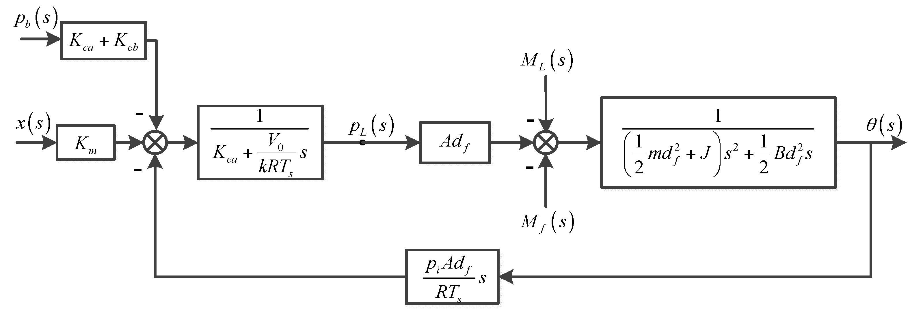
The block diagram of the pneumatic rotary actuator system, shown in Figure 4, can be obtained by Equations (21)–(23).

The transfer function of the pneumatic rotary actuator system can be derived directly by the block diagram:

(1)

After setting load moment $M_L$, friction moment $M_f$, and $p_b$ to zero, we obtain the transfer function from the displacement x of proportional valve spool to the output angle θ of pneumatic rotary actuator, which can be simplified as:

$$\frac{{\theta }_x\left(s\right)}{x\left(s\right)}=\frac{K_T}{s\left(\frac{{\mathrm{s}}^2}{{\omega }_0^2}+\frac{2\zeta }{{\omega }_0}s+1\right)}$$

(24)

where: gain

$$K_T=\frac{2K_{m}AR{T}_s}{B{d}_f{K}_{ca}R{T}_s+2A^2{d}_f{p}_i},$$

(25)

natural frequency

$${\omega }_0=\sqrt{\frac{B{d}_f^2{K}_{ca}kR{T}_s+2k{A}^2{d}_f^2{p}_i}{\left(m{d}_f^2+2J\right)V_0}},$$

(26)

and damping ratio

$$\zeta =\frac{K_{ca}kR{T}_s\left(m{d}_f^2+2J\right)+B{d}_f^2{V}_0}{2\sqrt{\left(m{d}_f^2+2J\right)\left(B{d}_f^2{K}_{ca}kR{T}_s+2k{A}^2{d}_f^2{p}_i\right)V_0}}$$

(27)

(2)

After setting displacement x of proportional valve spool and $p_b$ to zero, we obtain the transfer function from $M_L+M_f$ to the output angle θ of pneumatic rotary actuator, which can be predigested as:

$$\frac{{\theta }_M\left(s\right)}{M_L\left(s\right)+M_f\left(s\right)}=-\frac{\frac{K_T}{K_{m}A{d}_f}\left(K_{ca}+\frac{V_0}{kR{T}_s}s\right)}{s\left(\frac{{\mathrm{s}}^2}{{\omega }_0^2}+\frac{2\zeta }{{\omega }_0}s+1\right)}.$$

(28)

(3)

After setting displacement x of proportional valve spool, load moment $M_L$ and friction moment $M_f$ to zero, we obtain the transfer function from the friction $p_b$ to the output angle θ of pneumatic rotary actuator, which can be simplified as

$$\frac{{\theta }_p\left(s\right)}{p_b\left(s\right)}=-\frac{\frac{K_T}{K_m}\left(K_{ca}+K_{cb}\right)}{s\left(\frac{{\mathrm{s}}^2}{{\omega }_0^2}+\frac{2\zeta }{{\omega }_0}s+1\right)}$$

(29)

(4)

Total output of the pneumatic rotary actuator system is

$$\theta \left(s\right)={\theta }_x\left(s\right)+{\theta }_M\left(s\right)+{\theta }_p\left(s\right)=\frac{K_{T}x\left(s\right)-\frac{K_T}{K_{m}A{d}_f}\left(K_{ca}+\frac{V_0}{kR{T}_s}s\right)\left[M_L\left(s\right)+M_f\left(s\right)\right]-\frac{K_T}{K_m}\left(K_{ca}+K_{cb}\right)p_b\left(s\right)}{s\left(\frac{{\mathrm{s}}^2}{{\omega }_0^2}+\frac{2\zeta }{{\omega }_0}s+1\right)}.$$

(30)

3.5. Transfer Function of Proportional Directional Control Valve and Servo Amplifier

The natural frequency of the proportional directional control valve is 5~7 times larger than that of pneumatic rotary actuator. Hence, the proportional directional control valve responds quickly. Generally, its impact on the system can be ignored, and its transfer function can be regarded as a proportional link [33], which can be expressed by Equation (31).

$$\frac{x\left(s\right)}{U\left(s\right)}=K_v$$

(31)

where $U\left(s\right)$ is the Laplace transform of the output voltage of servo amplifier; $K_v$ is gain of proportional directional control valve.

The transfer function of the servo amplifier can be described as follows:

$$\frac{U\left(s\right)}{{\theta }_r\left(s\right)-\theta \left(s\right)}=K_a$$

(32)

where ${\theta }_r\left(s\right)$ is the Laplace transform of the system input angle; $K_a$ is gain of servo amplifier.

3.6. Transfer Function of the System

From Equations (30)–(32), the block diagram of the servo system shown in Figure 5 can be obtained.

Then the open-loop transfer function of the system can be obtained by the block diagram of the pneumatic rotary actuator servo system.

$$G\left(s\right)=\frac{K_a{K}_v{K}_T}{s\left(\frac{{\mathrm{s}}^2}{{\omega }_0^2}+\frac{2\zeta }{{\omega }_0}s+1\right)}$$

(33)

The initial parameter values of the model can be obtained, and shown in

Table 2. Values of model parameters.

Parameter	Value	Parameter	Value
A	3.4636 × 10−4 [m2]	m	0.21 [kg]
B	228 [N·s/m]	pe	1.013 × 105 [Pa]
C	0.68	R	287 [J/(kg·K)]
c0	0.21	Ts	293 [K]
df	0.014 [m]	V0	1.6767 × 10−5 [m3]
J	1.678 × 10−4 [kg·m2]	W	3.1415 × 10−2 [m]
k	1.4	x0	5 × 10−6 [m]

.

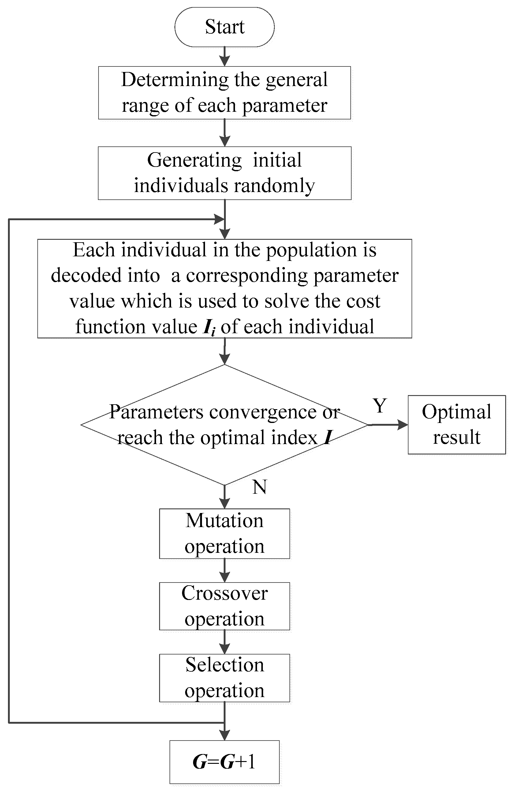
4. Adaptive Differential Evolution (ADE) Algorithm

Differential Evolution (DE) algorithm is a global optimization method based on swarm intelligence, which intelligently optimizes the evolution of the population through mutation, crossover and selection among individuals [34]. The idea of Differential Evolution (DE) algorithm is [35]: the initial individuals are randomly generated in the population, and the vector difference between any two individuals in the population is calculated; the vector difference is weighted according to a certain rule and summed up with the third individual to generate a new individual; if the fitness of the new individual is better than the target individual, the new individual will be used instead of the target individual to enter the next generation; otherwise, the old individual will continue the calculation of the next generation, so that the result will approximate to the optimal solution through the above iterative operation.

Adaptive Differential Evolution (ADE) algorithm ameliorates the scaling factor and crossover probability so that they can be adaptively changed during the iterative process, which improves the convergence precision and speeds up the convergence [36]. Since Adaptive Differential Evolution (ADE) algorithm has fewer parameters, strong global convergence and rapid convergence [37], it is suitable for the parameters tuning of pneumatic rotary actuator servo system.

Adaptive Differential Evolution (ADE) algorithm contains the following four steps.

4.1. Generating the Initial Population

The population contains $N_p$ D-dimensional vectors, whose parameters are real numbers. The i-th vector of the g-th generation can be marked as ${\mathit{x}}_{i,g}$. i = 1, 2, 3…N_p, g = 1, 2, 3…G, where G is the maximum generation. ${\mathit{x}}_{i,g}=\left(x_{j,i,g}\right)$, j = 1, 2, 3…D, where $x_{j,i,g}$ is j-th parameter of i-th vector.

The parent vector parameters $x_{j,i,0}$ are randomly generated and can be described by Equation (34).

$$x_{j,i,0}=ran{d}_j\left(0,1\right)\cdot \left(b_j^U-b_j^L\right)+b_j^L$$

(34)

where $ran{d}_j\left(0,1\right)$ is the random number generated in the interval [0, 1]; $b_j^U$ and $b_j^L$ are two D-dimensional initial vectors. The superscripts $U$ and $L$ denote the upper bound and lower bound, respectively.

4.2. Mutation Operation

After initialization, a population consisting of $N_p$ test vectors is produced by mutating the parent population. The mutation operation is to add a scalable difference between two randomly selected vectors to a third vector. Equation (35) shows how to combine three different and randomly selected vectors to produce a mutant vector ${\mathit{v}}_{i,g}$.

$${\mathit{v}}_{i,g}={\mathit{v}}_{r0,g}+F\cdot \left({\mathit{v}}_{r1,g}-{\mathit{v}}_{r2,g}\right)$$

(35)

where random indexes $r_0$, $r_1$, $r_2$$\in \left\{1,2,\mathrm{3...}{N}_p\right\}$.

We adjust the value of the scaling factor $F$ with a diminishing concave function. In the early stage of the algorithm, the value of $F$ is larger, and there is a larger population space, so the local extremum is not easy to appear and the convergence precision is improved. In the latter part of the algorithm, the value of $F$ is smaller, which helps to converge rapidly in the best range and increase the convergence rate [38]. The scaling factor $F$ can be given as:

$$F=\left(F_{\max }-F_{\min }\right){\left(\frac{G-g}{G}\right)}^2+F_{\min }$$

(36)

where $F_{\max }$ is the maximum value of $F$; $F_{\min }$ is the minimum value of $F$.

Merging Equations (36) and (35) yields:

$${\mathit{v}}_{i,g}={\mathit{v}}_{r0,g}+\left[\left(F_{\max }-F_{\min }\right){\left(\frac{G-g}{G}\right)}^2+F_{\min }\right]\left({\mathit{v}}_{r1,g}-{\mathit{v}}_{r2,g}\right).$$

(37)

4.3. Crossover Operation

Cross operation makes use of the parameters copied from two different vectors to form the test vector ${\mathit{u}}_{i,g}$. Cross operation compares the results of crossover probability $CR$ to a uniform random number generator $ran{d}_j\left(0,1\right)$. If the random number is less than or equal to $CR$, the test parameter will inherit the mutant vector ${\mathit{v}}_{i,g}$, otherwise the parameter will be copied from the vector ${\mathit{x}}_{i,g}$. Cross operation can be described by:

$${\mathit{u}}_{i,g}=u_{j,i,g}=\{\begin{array}{l}{v}_{j,i,g},ran{d}_j\left(0,1\right)\le CR\\ x_{j,i,g},ran{d}_j\left(0,1\right)>CR\end{array}$$

(38)

where $v_{j,i,g}$ is j-th parameter of i-th mutant vector, $u_{j,i,g}$ is j-th parameter of i-th test vector.

We use an increasing convex function to adjust the crossover probability, $CR$. In the initial stage of the algorithm, $CR$ has a smaller value, and there is a larger population space, which improves the global convergence capability. In the latter part of the algorithm, $CR$ takes a larger value and improves the convergence speed. The crossover probability, $CR$, can be given as:

$$CR=C{R}_{\min }+\left(C{R}_{\max }-C{R}_{\min }\right){\left(\frac{g}{G}\right)}^2$$

(39)

where $C{R}_{\max }$ is the maximum value of $CR$; $C{R}_{\min }$ is the minimum value of $CR$.

4.4. Selection Operation

If the target function value of the test vector is less than or equal to the target function value of the target vector, the test vector will enter the next generation, otherwise the target vector will enter the next generation. The target function can be represented by the symbol $f_c$. So the number of vectors remains unchanged, and the fitness will be better or remain the same. The selection operation process can be expressed as follows:

$${\mathit{x}}_{i,g+1}=\{\begin{array}{l}{\mathit{u}}_{i,g},f_c\left({\mathit{u}}_{i,g}\right)<f_c\left({\mathit{x}}_{i,g}\right)\\ {\mathit{x}}_{i,g},\mathrm{else}\end{array}.$$

(40)

Operations of mutation, crossover, and selection were circulated in turn until the maximum number of evolutionary iterations, $G$, was reached.

5. ADE-PD Controller Design

The PD controller can make the system respond quickly and have little lag. So, it is used to optimize the control of the pneumatic rotary actuator servo system, and the parameters $k_p$ and $k_d$ of PD controller are tuned by Adaptive Differential Evolution (ADE) algorithm [39]. The first order low pass filter is also used in the system in order to reduce other interferences of the measurement channel and ensure the stability of the deviation $e\left(n\right)$. The schematic diagram of the control system with the ADE-PD controller is shown in Figure 6. The controller can be expressed in a time-discrete way [40].

The relationship between the input and output signals of the first order low pass filter is:

$$e\prime \left(n\right)=\left(1-\alpha \right)e\prime \left(n-1\right)+\alpha e\left(n\right)$$

(41)

where $e\left(n\right)$ and $e\prime \left(n\right)$ are input and output of the filter at the n-th sampling, n = 1, 2, 3…; filter coefficient $\alpha =1-e^{-T_P/\tau }$, where $T_P$ is sampling period, and $\tau$ is time constant.

The discrete PD algorithm can be expressed as:

$$z\left(n\right)=k_p\left\{e\prime \left(n\right)+\frac{T_d}{T_P}\left[e\prime \left(n\right)-e\prime \left(n-1\right)\right]\right\}=k_{p}e\prime \left(n\right)+k_d\left[e\prime \left(n\right)-e\prime \left(n-1\right)\right]$$

(42)

where $z\left(n\right)$ is output of the controller, $T_d$ is differential time constant, $k_p$ is proportional coefficient, and $k_d$ is differential coefficient, $k_d=k_p{T}_d/T_P$.

In order to obtain the satisfactory dynamic characteristics of the transient process, the discrete integral of time-weighted absolute value of the error (ITAE) is used as the minimum target function of the parameter selection. The square of the input is added to the target function, so as to prevent excessive control. The optimal index in the process of optimizing parameters $k_p$ and $k_d$ is given as:

$$I={\displaystyle \sum _{n=1}^Z\left[w_1\left|e\prime \left(n\right)\right|+w_2{\theta }_r^2\left(n\right)\right]T_P}$$

(43)

where $Z$ is total points of sampling; $w_1$ and $w_2$ are weights.

In order to avoid overshoot, the penalty function is used, that is, once the overshoot is produced, the overshoot is added as one part of the optimal index. At this time, the optimal index is:

$$\mathrm{when} e\prime \left(n\right)<0,I={\displaystyle \sum _{n=1}^Z\left[w_1\left|e\prime \left(n\right)\right|+w_2{\theta }_r^2\left(n\right)+w_3\left|e\prime \left(n\right)\right|\right]}{T}_P$$

(44)

where $w_3$ is weight, $w_3\gg w_1$.

The flowchart of optimizing parameters with Adaptive Differential Evolution (ADE) algorithm is described in Figure 7.

6. Experiment and Analysis

The supply pressure of the experiment is 0.6 MPa, and the gas temperature is 20 °C. We select some parameters which are suitable for this system. The number of individuals is 30, the proportional coefficient $k_p$ is in the interval [−5, 20], the range of the differential coefficient $k_d$ is [−1, 1], where adding ranges of negative numbers can lead to better iterative processes, and cannot affect final results that are positive. The weights $w_1$ = 0.999, $w_2$ = 0.001, and $w_3$ = 10, and the evolutionary iterations G = 50. Sampling period $T_P$ is 1 ms.

6.1. Parameters Selection and Comparison with DE Algorithms

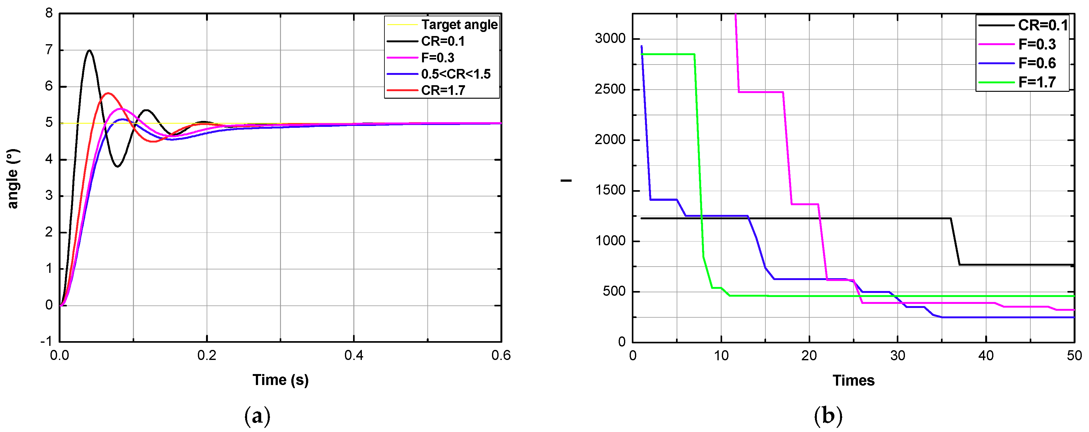
The DE-PD controller is used to control the system in the experiment firstly. When crossover probability $CR$ is set to 0.6, we can obtain different trajectory curves of pneumatic rotary actuator by changing the value of scaling factor $F$ to analyze the influence of parameter $F$ on the system. Figure 8 shows different results of rotation positions of the actuator and cost functions I_i when $F$ = 0.04, 0.05–1.4, 1.6, and 1.8. It can be observed from Figure 8a that the overshoot and fluctuation of position curve are the least and almost unchanged when $F$ is 0.05~1.4. Overly high or low $F$ can affect the stability of the trajectory. Figure 8b reveals different convergent processes when $F$ changes, and it verifies that the higher $F$ is, the slower the convergence rate is.

In the same way, different trajectory curves are shown in Figure 9a when $CR$ = 0.1, 0.3, 0.5~1.5, and 1.7 after $F$ is set to 1.0. In the interval of $CR$ [0.5,1.5], the overshoot and fluctuation of position curve are the least, and there are large fluctuations of rotation with other values of $CR$. From Figure 9b, we can also conclude that larger $CR$ can make the convergence faster.

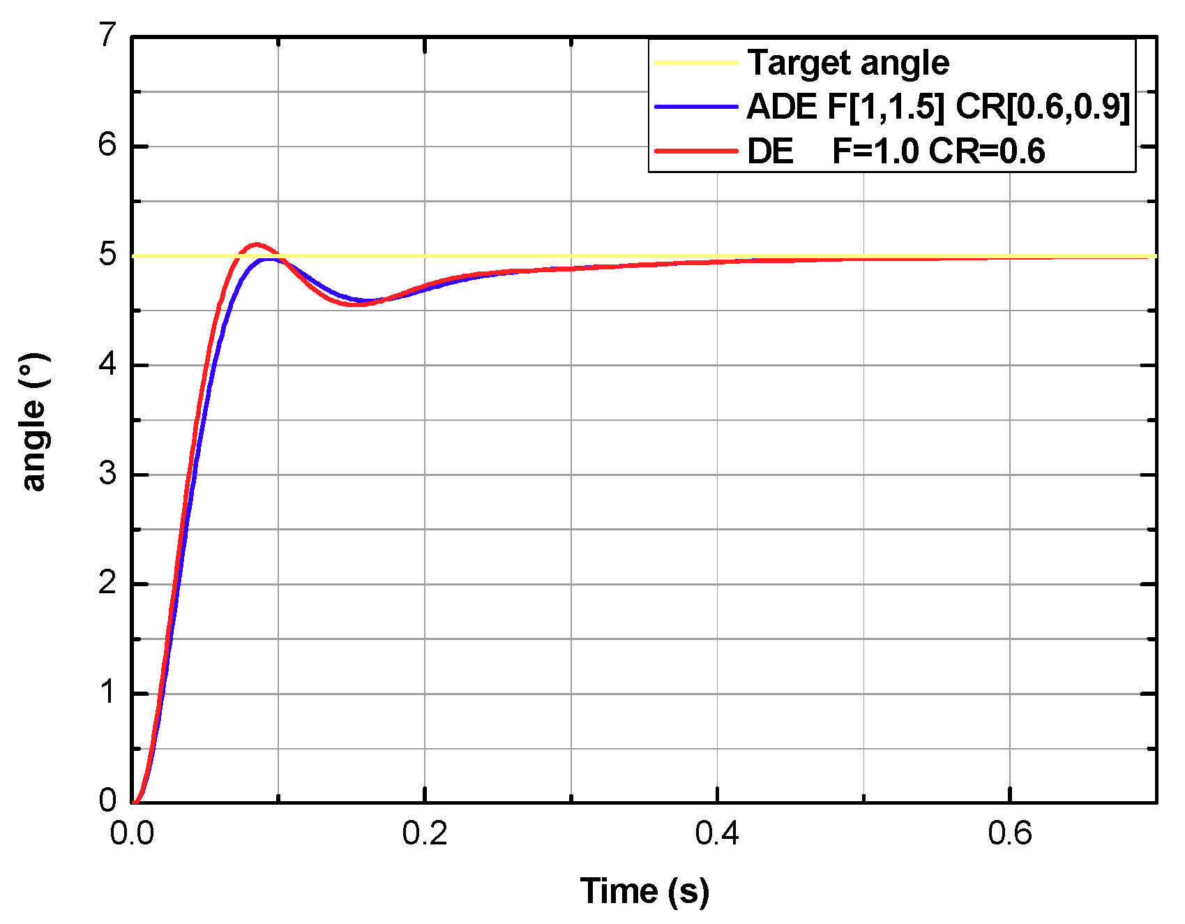
Then another experiment is done with ADE-PD control by changing $F_{\max }$, $F_{\min }$, $C{R}_{\max }$, and $C{R}_{\min }$. Figure 10 shows different rotation positions with ADE-PD control and the trajectory of the actuator performs best when $F_{\max }$ = 1.5, $F_{\min }$ = 1.0, $C{R}_{\max }$ = 0.9, and $C{R}_{\min }$ = 0.6. We compare the curves controlled by ADE and DE in Figure 11, and come to a conclusion that position curve controlled by ADE-PD has smaller overshoot and fluctuation.

6.2. Comparison with NCD-PID Control

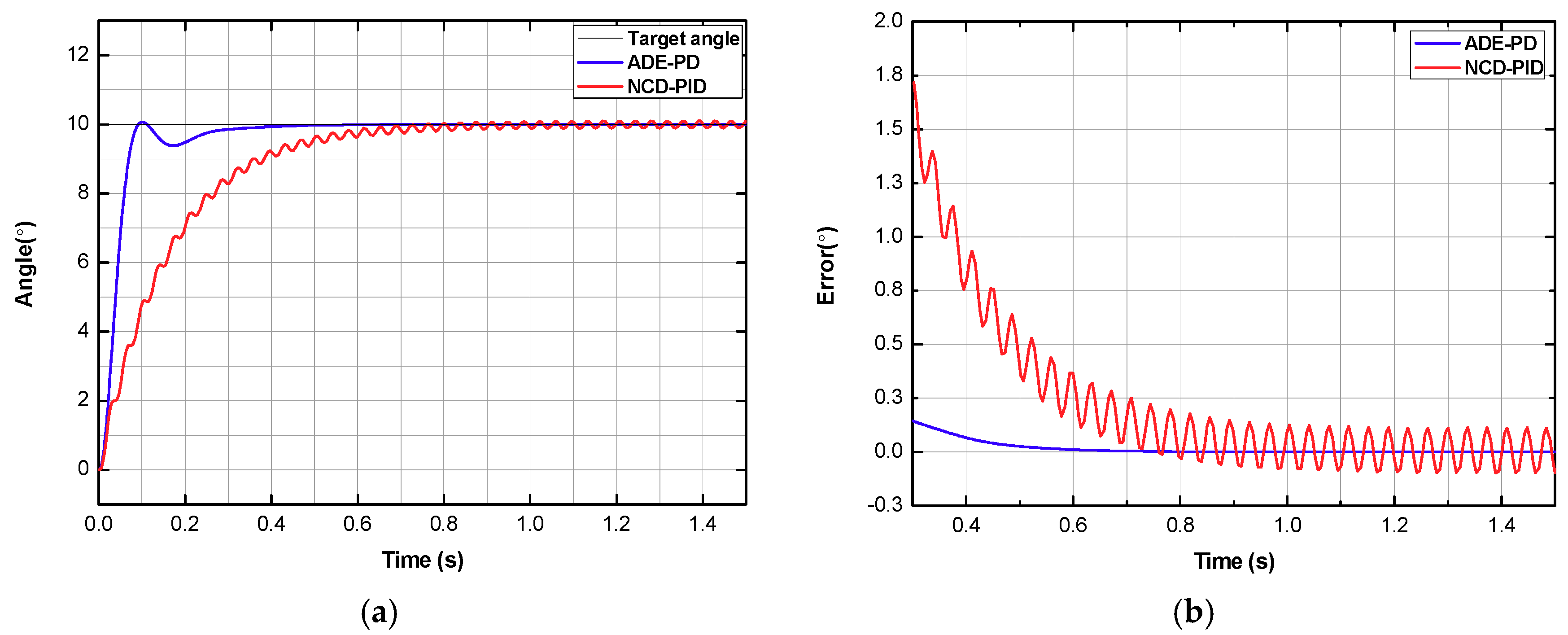
In the experiment, the PID controller optimized by NCD is also used to control rotation position and is compared with the ADE-PD controller. Firstly, the target angle is set as 10°. As shown in Figure 12, the response curve controlled by ADE-PD controller reaches peak in 0.101 s, and reaches the steady state in 0.355 s, and the steady state error is controlled within 0.1°. However, the peak time of the response curve controlled by NCD-PID controller is 0.95 s, and at the same time, the steady state error is 0.15°, and there are slight fluctuations throughout the process. So system based on ADE-PD control has greater position precision and faster response.

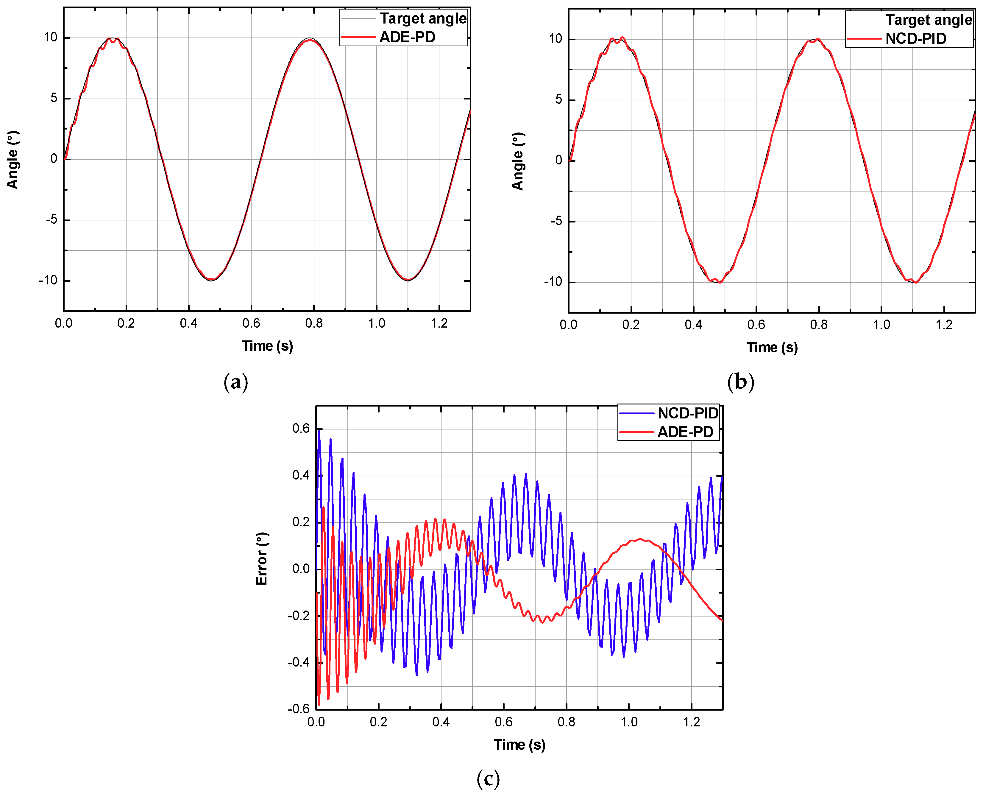
If the input signals are changed to sinusoidal waves with different frequencies, we can obtain the trackings of the position. Figure 13, Figure 14 and Figure 15 show comparisons of tracking curves when the frequency of sinusoidal signal is 5 rad/s, 10 rad/s, and 3 rad/s, respectively. As shown in Figure 13c, steady state error controlled by ADE-PD is 0.06°, while the error controlled by NCD-PID is 0.25°. In Figure 14c, the steady state error controlled by ADE-PD is 0.22°, and the error controlled by NCD-PID is 0.41°. Finally, the steady state error controlled by ADE-PD is 0.04°, while the error controlled by NCD-PID is 0.17° in Figure 15c.

By contrasting the errors in Figure 13c, Figure 14c andFigure 15c, we come to a conclusion that the control precision of the system becomes worse with the increase of the frequency of sinusoidal wave. And in Figure 12a, Figure 13b, Figure 14b and Figure 15b, there are persistent fluctuations in steady state because of stickiness in the actuator when changing the direction of motion. The system based on ADE-PD control can reduce the occurrence of stickiness and has less errors and fluctuations as shown in Figure 12b, Figure 13c, Figure 14c andFigure 15c.

6.3. Discussion on Increasing Inertia Load

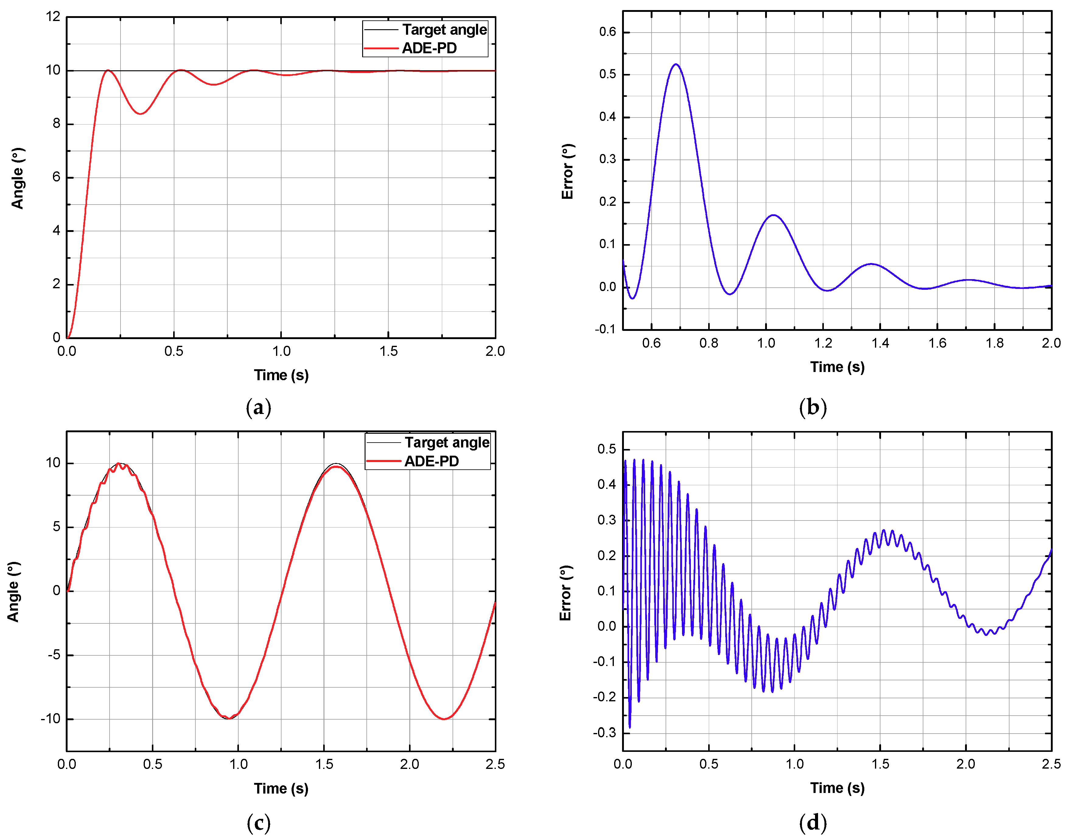
The moment of inertia of the pneumatic rotary actuator itself is 1.678 × 10⁻⁴ kg·m², which can be increased by loading block on rotating platform. Tracking curves are shown in Figure 16 when moment of inertia is 3.2 × 10⁻⁴ kg·m², and the curves are shown in Figure 17 when moment of inertia is 4.5 × 10⁻⁴ kg·m². Figure 16a,b describe rotation positions tracking fixed value, while Figure 17a,b provide rotation positions tracking sinusoidal signal whose frequency is 5 rad/s.

From the results in Figure 12b, Figure 16b, and Figure 17b, we summarize that increasing the inertia load can increase the rotation fluctuation and error. And it can be observed from Equations (25) and (26) that increasing the moment of inertia will reduce natural frequency and damping ratio. Thereby it makes the error increase and even deviate from center, which is obtained from Figure 13c, Figure 16d, and Figure 17d. Even so, the system has relatively stable trajectories and tiny errors which are within 0.27°, and shows good robustness.

7. Conclusions

In this paper, the pneumatic rotary actuator position servo system is studied and analyzed, and an experimental platform is set up. The motion laws of the rack and pinion pneumatic rotary actuator and the proportional directional control valve are analyzed. Starting from the flow of gas flowing through the proportional directional control valve and the motion state of the pneumatic rotary actuator, the basic equations of the actuator controlled by the valve are obtained and linearized near the middle position, and the mathematical model of the pneumatic rotary actuator is deduced. Then the mathematical model of the whole system is obtained. The establishment of this model lays a foundation for the research of theory and experiment.

An Adaptive Differential Evolution (ADE) algorithm is proposed in this paper. In the process of individual variation, the values of scaling factor and crossover probability are adjusted by a decreasing concave function and an increasing convex function, respectively, which improves the accuracy and the speed of algorithm optimization. The ADE-PD controller is designed to control the pneumatic rotary actuator position servo system, and the experimental platform is used to select parameters, compare the controller with DE algorithm, and compare with PID controller by changing input signals. Finally, the characteristics of the system are discussed by increasing the inertia load. The conclusions obtained from experiments can be summarized as follows:

(a)

Different values of $F$ and $CR$ can change the stability of the control. Rotation position controlled by ADE-PD has smaller overshoot and fluctuation than others controlled by DE-PD when $F_{\max }$ = 1.5, $F_{\min }$ = 1.0, $C{R}_{\max }$ = 0.9, $C{R}_{\min }$ = 0.6.

(b)

The control precision of the system becomes worse with the increase of the frequency of sinusoidal wave. And there are persistent fluctuations in steady state because of stickiness in the actuator when changing the direction of motion. The system based on ADE-PD control can reduce the occurrence of stickiness, and has greater position precision and faster response than NCD-PID control.

(c)

Increasing the moment of inertia will reduce natural frequency and damping ratio, and make the error increase and even deviate from center. Even so, the system has relatively stable trajectories and tiny errors, which shows great robustness.

(d)

Although a resonance is expected by the compressibility and the friction could cause a small displacement instability, a reasonable control can be obtained.

References

- Zhang, Y.; Cai, M. Whole life-cycle costing analysis of pneumatic actuators. J. Beijing Univ. Aeronaut. Astronaut. 2011, 37, 1006–1010. [Google Scholar]
- Yang, F.; Tadano, K.; Li, G.; Kagawa, T. Analysis of the energy efficiency of a pneumatic booster regulator with energy recovery. Appl. Sci. 2017, 7, 816. [Google Scholar] [CrossRef]
- Zhang, Y.M.; Cai, M.L. Overall life cycle comprehensive assessment of pneumatic and electric actuator. Chin. J. Mech. Eng. (Engl. Ed.) 2014, 27, 584–594. [Google Scholar] [CrossRef]
- Zang, X.; Liu, Y.; Li, W.; Lin, Z.; Zhao, J. Design and experimental development of a pneumatic stiffness adjustable foot system for biped robots adaptable to bumps on the ground. Appl. Sci. 2017, 7, 1005. [Google Scholar] [CrossRef]
- Jiang, G.; Luo, M.; Bai, K.; Chen, S. A precise positioning method for a puncture robot based on a PSO-optimized BP neural network algorithm. Appl. Sci. 2017, 7, 969. [Google Scholar] [CrossRef]
- Sheng, Z.; Li, Y. Hybrid robust control law with disturbance observer for high-frequency response electro-hydraulic servo loading system. Appl. Sci. 2016, 6, 98. [Google Scholar] [CrossRef]
- Pujana-Arrese, A.; Mendizabal, A.; Arenas, J.; Prestamero, R.; Landaluze, J. Modelling in modelica and position control of a 1-DoF set-up powered by pneumatic muscles. Mechatronics 2010, 20, 535–552. [Google Scholar] [CrossRef]
- Niu, J.; Shi, Y.; Cao, Z.; Cai, M.; Chen, W.; Zhu, J.; Xu, W. Study on air flow dynamic characteristic of mechanical ventilation of a lung simulator. Sci. China Technol. Sci. 2017, 60, 243–250. [Google Scholar] [CrossRef]
- Ren, S.; Shi, Y.; Cai, M.; Xu, W. Influence of secretion on airflow dynamics of mechanical ventilated respiratory system. IEEE/ACM Trans. Comput. Biol. Bioinform. 2017, 99, 1. [Google Scholar] [CrossRef] [PubMed]
- Ren, S.; Shi, Y.; Cai, M.; Xu, W.; Zhang, X.D. Influence of bronchial diameter change on the airflow dynamics based on a pressure-controlled ventilation system. Int. J. Numer. Method Biomed. Eng. 2017. [Google Scholar] [CrossRef] [PubMed]
- Saravanakumar, D.; Mohan, B.; Muthuramalingam, T. A review on recent research trends in servo pneumatic positioning systems. Precis. Eng. J. Int. Soc. Precis. Eng. Nanotechnol. 2017, 49, 481–492. [Google Scholar] [CrossRef]
- Rad, C.-R.; Hancu, O. An improved nonlinear modelling and identification methodology of a servo-pneumatic actuating system with complex internal design for high-accuracy motion control applications. Simul. Model. Pract. Theory 2017, 75, 29–47. [Google Scholar] [CrossRef]
- Ren, H.; Fan, J. Adaptive backstepping slide mode control of pneumatic position servo system. Chin. J. Mech. Eng. (Engl. Ed.) 2016, 29, 1003–1009. [Google Scholar] [CrossRef]
- Shi, Y.; Wang, Y.; Cai, M.; Zhang, B.; Zhu, J. An aviation oxygen supply system based on a mechanical ventilation model. Chin. J. Aeronaut. 2017, 31, 197–204. [Google Scholar] [CrossRef]
- Shi, Y.; Zhang, B.; Cai, M.; Xu, W. Coupling effect of double lungs on a VCV ventilator with automatic secretion clearance function. IEEE/ACM Trans. Comput. Biol. Bioinform. 2017, 99, 1. [Google Scholar] [CrossRef] [PubMed]
- Shi, Y.; Wu, T.; Cai, M.; Wang, Y.; Xu, W. Energy conversion characteristics of a hydropneumatic transformer in a sustainable-energy vehicle. Appl. Energy 2016, 171, 77–85. [Google Scholar] [CrossRef]
- Shi, Y.; Wang, Y.; Liang, H.; Cai, M. Power characteristics of a new kind of air-powered vehicle. Int. J. Energy Res. 2016, 40, 1112–1121. [Google Scholar] [CrossRef]
- Bai, Y.H. Research on Pneumatic Rotation Position Servo Control Technology. Ph.D. Thesis, Nanjing University of Science and Technology, Nanjing, China, 2006. [Google Scholar]
- Thanh, T.U.D.C.; Ahn, K.K. Nonlinear PID control to improve the control performance of 2 axes pneumatic artificial muscle manipulator using neural network. Mechatronics 2006, 16, 577–587. [Google Scholar] [CrossRef]
- Zhang, Y.; Cai, M.; Kong, D. Overall energy efficiency of lubricant-injected rotary screw compressors and aftercoolers. In Proceedings of the IEEE Computer Society 2009 Asia-Pacific Power and Energy Engineering Conference (APPEEC 2009), Wuhan, China, 27–31 March 2009; Chinese Society for Electrical Engineering; IEEE Power and Energy Society; Scientific Research Publishing; Wuhan University: Wuhan, China, 2009. [Google Scholar]
- Lin, T.; Chen, Q.; Ren, H.; Zhao, Y.; Miao, C.; Fu, S.; Chen, Q. Energy regeneration hydraulic system via a relief valve with energy regeneration unit. Appl. Sci. 2017, 7, 613. [Google Scholar] [CrossRef]
- Kagawa, T.; Cai, M.; Kameya, H. Overall efficiency consideration of pneumatic systems including compressor, dryer, pipe and actuator. In Proceedings of the JFPS International Symposium on Fluid Power 2002, Nara, Japan, 12–15 November 2002; pp. 383–388. [Google Scholar]
- Shi, Y.; Zhang, B.; Cai, M.; Zhang, X.D. Numerical simulation of volume-controlled mechanical ventilated respiratory system with 2 different lungs. Int. J. Numer. Method Biomed. Eng. 2016, 33, 2852. [Google Scholar] [CrossRef] [PubMed]
- Gai, Y.; Cai, M.; Shi, Y. Analytical and experimental study on complex compressed air pipe network. Chin. J. Mech. Eng. (Engl. Ed.) 2015, 28, 1023–1029. [Google Scholar] [CrossRef]
- Kaitwanidvilai, S.; Parnichkun, M. Position control of a pneumatic servo system by genetic algorithm based fixed-structure robust h, loop shaping control. In Proceedings of the IECON 2004—30th Annual Conference of IEEE Industrial Electronics Society, Busan, Korea, 2–6 November 2004; IEEE Computer Society: Busan, Korea, 2004; pp. 2246–2251. [Google Scholar]
- Li, J.P. Pneumatic Transmission System Dynamics; South China University of Technology Press: Guangzhou, China, 1991; pp. 32–35. ISBN 7562302677. [Google Scholar]
- Yin, Y.B. High Speed Pneumatic Theory and Technology; Shanghai Science and Technology Press: Shanghai, China, 2014; pp. 165–171. ISBN 978-7-5478-2068-1. [Google Scholar]
- Ning, F.; Shi, Y.; Cai, M.; Wang, Y.; Xu, W. Research progress of related technologies of electric-pneumatic pressure proportional valves. Appl. Sci. 2017, 7, 1074. [Google Scholar] [CrossRef]
- Shi, Y.; Ren, S.; Cai, M.; Xu, W.; Deng, Q. Pressure dynamic characteristics of pressure controlled ventilation system of a lung simulator. Comput. Math. Methods Med. 2014, 761712–761722. [Google Scholar] [CrossRef] [PubMed]
- Shearer, J.L. Study of pneumatic processes in the continuous control of motion with compressed air-I. Trans. ASME 1956, 2, 233–242. [Google Scholar]
- Wu, Z.S. Pneumatic Transmission and Control, 2nd ed.; Harbin Institute of Technology Press: Harbin, China, 2009; pp. 197–199. ISBN 7-5603-0989-5. [Google Scholar]
- Cai, M.; Wang, Y.; Shi, Y.; Liang, H. Output dynamic control of a late model sustainable energy automobile system with nonlinearity. Adv. Mech. Eng. 2016, 8. [Google Scholar] [CrossRef]
- Yang, Z.R.; Hua, K.Q.; Xu, Y. Electro-Hydraulic Ratio and Servo Control; Metallurgical Industry Press: Beijing, China, 2015; pp. 108–120. ISBN 978-7-5024-4622-2. [Google Scholar]
- Storn, R.; Price, K. Differential evolution—A simple and efficient heuristic for global optimization over continuous spaces. J. Glob. Optim. 1997, 11, 341–359. [Google Scholar] [CrossRef]
- Wu, L.; Wang, Y.; Zhou, S.; Tan, W. Design of PID controller with incomplete derivation based on differential evolution algorithm. J. Syst. Eng. Electron. 2008, 19, 578–583. [Google Scholar]
- Zhang, X.; Zhang, X. Shift based adaptive differential evolution for PID controller designs using swarm intelligence algorithm. Clust. Comput. 2017, 20, 291–299. [Google Scholar] [CrossRef]
- Liu, J.K. Advanced Pid Control Matlab Simulation, 4th ed.; Publishing House of Electronics Industry: Beijing, China, 2016; pp. 331–332. ISBN 978-7-121-28846-3. [Google Scholar]
- Cheng, L.; Chen, J.; Chen, M.; Xu, J.; Wang, W.; Wang, T.; Guo, J. Adaptive differential evolution algorithm identification of photoelectric tracking servo system. Hongwai Yu Jiguang Gongcheng Infrared Laser Eng. 2016, 45. [Google Scholar] [CrossRef]
- Andromeda, T.; Yahya, A.; Samion, S.; Baharom, A.; Hashim, N.L. Differential evolution for optimization of PID gain in electrical discharge machining control system. Trans. Can. Soc. Mech. Eng. 2013, 37, 293–301. [Google Scholar]
- Niu, J.; Shi, Y.; Cai, M.; Cao, Z.; Wang, D.; Zhang, Z.; Zhang, X.D. Detection of sputum by interpreting the time-frequency distribution of respiratory sound signal using image processing techniques. Bioinformatics 2018, 34, 820–827. [Google Scholar] [CrossRef] [PubMed]
Figure 1.
Schematic diagram of pneumatic rotary actuator position servo system (1—Air compressor; 2—Air filter; 3—Air regulator; 4—Air lubricator; 5—Proportional directional control valve; 6—Rotary encoder; 7—Rack and pinion pneumatic rotary actuator; and 8—IPC).
Figure 2.
Experimental platform of pneumatic rotary actuator position servo system.
Figure 3.
Schematic diagram of the valve-controlled actuator.
Figure 4.
Block diagram of the pneumatic rotary actuator system.
Figure 5.
Block diagram of the pneumatic rotary actuator servo system.
Figure 6.
Schematic diagram of control system with ADE-PD controller.
Figure 7.
Flow chart of parameter tuning of ADE-PD controller.
Figure 8.
Comparison of experimental results with changed F, (a) Rotation positions; (b) Cost functions Ii.
Figure 9.
Comparison of experimental results with changed CR, (a) Rotation positions; (b) Cost functions Ii.
Figure 10.
Different rotation positions with ADE-PD control.
Figure 11.
Comparison of curves controlled by ADE-PD and DE-PD.
Figure 12.
Comparison of curves controlled by ADE-PD and NCD-PID: (a) Rotation positions and (b) Errors.
Figure 13.
Comparison of tracking curves when the frequency of sinusoidal signal is 5 rad/s: (a) Tracking curve controlled by ADE-PD; (b) Tracking curve controlled by NCD-PID; and (c) Errors.
Figure 14.
Comparison of tracking curves when the frequency of sinusoidal signal is 10 rad/s: (a) Tracking curve controlled by ADE-PD; (b) Tracking curve controlled by NCD-PID; and (c) Errors.
Figure 15.
Figure 16.
Tracking curves when moment of inertia is 3.2 × 10⁻⁴ kg·m2: (a) Rotation position tracking fixed value; (b) Error tracking fixed value; (c) Rotation position tracking sinusoidal signal; and (d) Error tracking sinusoidal signal.
Figure 17.
Tracking curves when moment of inertia is 4.5 × 10⁻⁴ kg·m2: (a) Rotation position tracking fixed value; (b) Error tracking fixed value; (c) Rotation position tracking sinusoidal signal; and (d) Error tracking sinusoidal signal.