Iterative 2D Tissue Motion Tracking in Ultrafast Ultrasound Imaging

 ,
,  ,
,
Abstract
:1. Introduction
2. Materials and Methods
2.1. Proposed Tracking Scheme
- First, the frame rate is temporarily down sampled by a factor k, where k = (2, 4, 8, 16, 32, 64, or 128). The position of each kernel is estimated with a Lagrangian viewpoint between every frame in the temporary cine loop (solid lines in Figure 1a). The position of the kernel in each frame is estimated using a block-matching method with an extra kernel described in [28] (where the method is denoted as the “basic method using an extra reference block”). This method was developed to minimize estimation errors when using a Lagrangian viewpoint.
- Iteratively: the frame rate is temporarily down sampled by a factor m = k/2i where i is the iteration number. The unknown kernel positions in each middle frame in the temporary cine loop are determined by the kernels from the anteroposterior frames (dashed lines in Figure 1b). The two independently estimated positions are averaged to determine the kernel position in the middle frame. The iterations continued until the position of the kernel is estimated in every frame (dashed lines in Figure 2c), i.e., m = 1. The position of the kernel is estimated using the block-matching method denoted “basic method” in [28].
2.2. Cine Loops
2.3. Evaluation of Motion Estimations
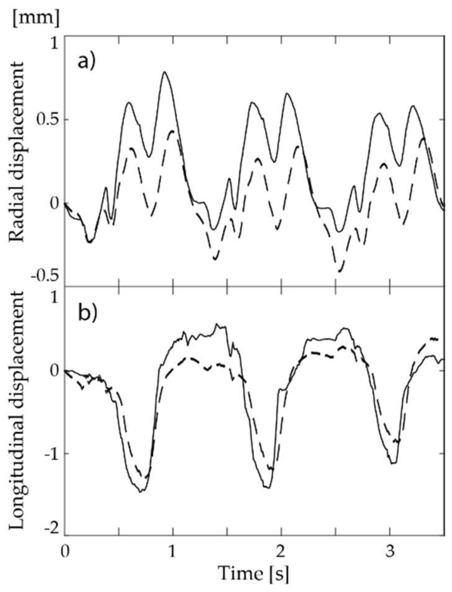
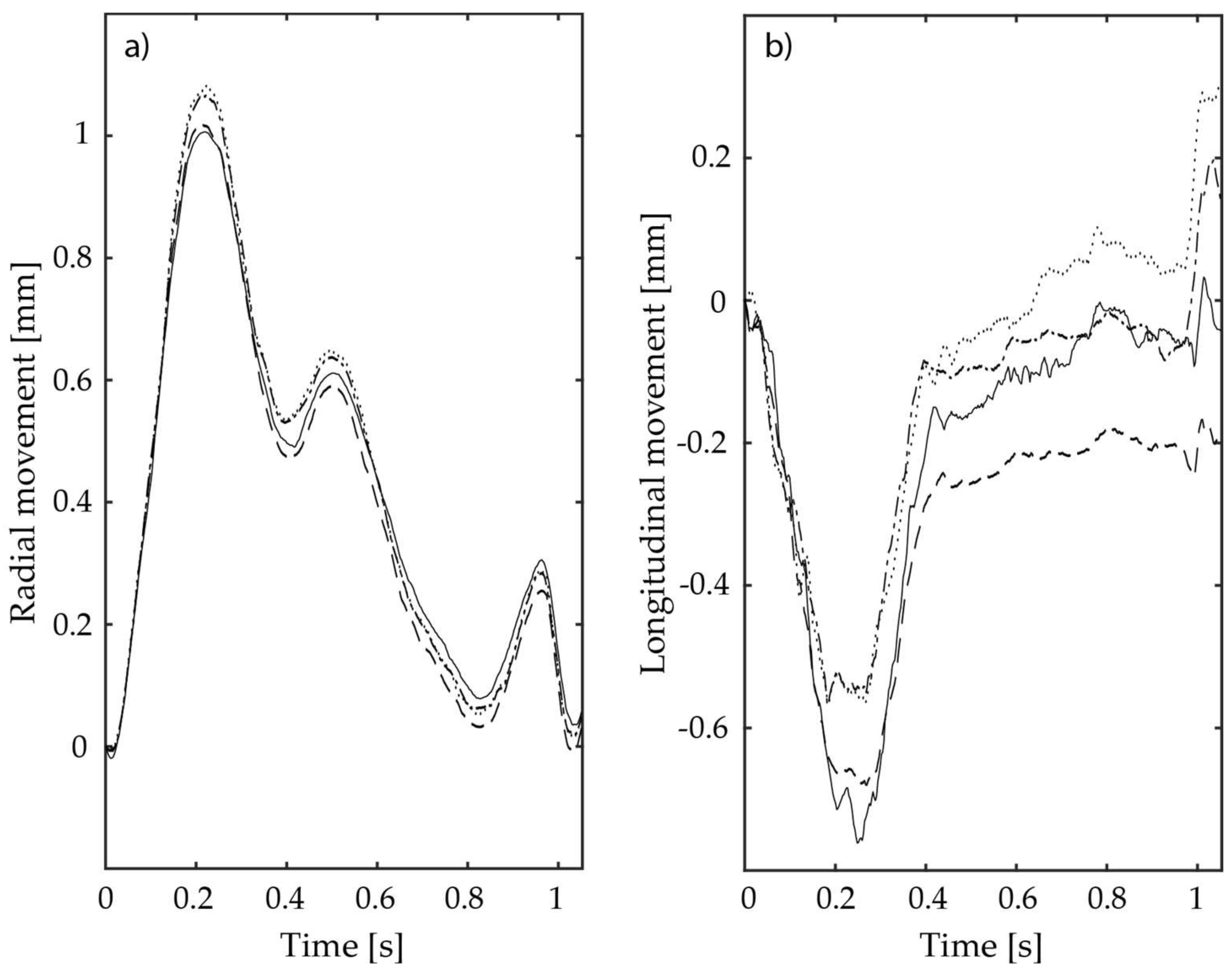
3. Results
4. Discussion
- Using a small initial length of iteration (k ≤ 2) gave rather small mean estimation errors but gave large standard deviations. Each of the motion estimations in the first iteration gave a very small error, but they accumulated to rather large errors and did so along different paths.
- Using a medium initial length of iteration (k = 4–32) gave larger mean estimation errors but smaller standard deviations. All estimations were roughly equal, but the initial motion estimations underestimated the motions. The later iterations gave accurate estimations for the in-between frames, but their starting points from the first iteration were incorrect.
- Using a large initial length of iteration (k ≥ 64) gave small mean estimation errors and small standard deviations. The distance moved between each frame in the first iteration was large enough for the motion estimations to be accurate and for the later iterations to give accurate estimations for the in-between frames.
5. Conclusions
Author Contributions
Acknowledgments
Conflicts of Interest
References
- Gennisson, J.-L.; Provost, J.; Deffieux, T.; Papadacci, C.; Imbault, M.; Pernot, M.; Tanter, M. 4-D Ultrafast Shear-Wave Imaging. IEEE Trans. Ultrason. Ferroelectr. Freq. Control 2015, 62, 1059–1065. [Google Scholar] [CrossRef] [PubMed]
- Bercoff, J.; Chaffai, S.; Tanter, M.; Sandrin, L.; Catheline, S.; Fink, M.; Gennisson, J.L.; Meunier, M. In Vivo Breast Tumor Detection using Transient Elastography. Ultrasound Med. Biol. 2003, 29, 1387–1396. [Google Scholar] [CrossRef]
- Muller, M.; Gennisson, J.-L.; Deffieux, T.; Tanter, M.; Fink, M. Quantitative Viscoelasticity Mapping of Human Liver using Supersonic Shear Imaging: Preliminary in Vivo Feasibility Study. Ultrasound Med. Biol. 2009, 35, 219–229. [Google Scholar] [CrossRef] [PubMed]
- Tanter, M.; Bercoff, J.; Sandrin, L.; Fink, M. Ultrafast Compound Imaging for 2-D Motion Vector Estimation: Application to Transient Elastography. IEEE Trans. Ultrason. Ferroelectr. Freq. Control 2002, 49, 1363–1374. [Google Scholar] [CrossRef] [PubMed]
- Palmeri, M.L.; Wang, M.H.; Dahl, J.J.; Frinkley, K.D.; Nightingale, K. Quantifying Hepatic Shear Modulus in Vivo using Acoustic Radiation Force. Ultrasound Med. Biol. 2008, 34, 546–558. [Google Scholar] [CrossRef] [PubMed]
- Hansen, P.M.; Olesen, J.B.; Pihl, M.J.; Lange, T.; Heerwagen, S.; Pedersen, M.M.; Rix, M.; Lönn, L.; Jensen, J.A.; Nielsen, M.B. Volume Flow in Arteriovenous Fistulas using Vector Velocity Ultrasound. Ultrasound Med. Biol. 2014, 40, 2707–2714. [Google Scholar] [CrossRef] [PubMed]
- Lenge, M.; Ramalli, A.; Boni, E.; Liebgott, H.; Cachard, C.; Tortoli, P. High-frame-rate 2-D vector blood flow imaging in the frequency domain. IEEE Trans. Ultrason. Ferroelectr. Freq. Control 2014, 61, 1504–1514. [Google Scholar] [CrossRef] [PubMed]
- Takahashi, H.; Hasegawa, H.; Kanai, H. Echo speckle imaging of blood particles with high-frame-rate echocardiography. Jpn. J. Appl. Phys. 2014, 53, 07KF08. [Google Scholar] [CrossRef]
- Deffieux, T.; Jean-Luc, G.; Tanter, M.; Fink, M. Assessment of the Mechanical Properties of the Musculoskeletal System Using 2-D and 3-D Very High Frame Rate Ultrasound. IEEE Trans. Ultrason. Ferroelectr. Freq. Control 2008, 55, 2177–2190. [Google Scholar] [CrossRef] [PubMed]
- Errico, C.; Osmanski, B.-F.; Pezet, S.; Couture, O.; Lenkei, Z.; Tanter, M. Transcranial functional ultrasound imaging of the brain using microbubble-enhanced ultrasensitive Doppler. NeuroImage 2016, 124, 752–761. [Google Scholar] [CrossRef] [PubMed]
- Tong, L.; Gao, H.; Choi, H.F.; D’hooge, J. Comparison of Conventional Parallel Beamforming With Plane Wave and Diverging Wave Imaging for Cardiac Applications: A Simulation Study. IEEE Trans. Ultrason. Ferroelectr. Freq. Control 2012, 59, 1654–1663. [Google Scholar] [CrossRef] [PubMed]
- Hasegawa, H.; Kanai, H. High-frame-rate echocardiography using diverging transmit beams and parallel receive beamforming. J. Med. Ultrason. 2011, 38, 129–140. [Google Scholar] [CrossRef] [PubMed]
- Hasegawa, H.; Kanai, H. Simultaneous imaging of artery-wall strain and blood flow by high frame rate acquisition of RF signals. IEEE Trans. Ultrason. Ferroelectr. Freq. Control 2008, 55, 2626–2639. [Google Scholar] [CrossRef] [PubMed]
- Salles, S.; Chee, A.J.Y.; Garcia, D.; Yu, A.C.H.; Vray, D.; Liebgott, H. 2-D Arterial Wall Motion Imaging Using Ultrafast Ultrasound and Transverse Oscillations. IEEE Trans. Ultrason. Ferroelectr. Freq. Control 2015, 62, 1047–1058. [Google Scholar] [CrossRef] [PubMed]
- Kruizinga, P.; Mastik, F.; van den Oord, S.C.H.; Schinkel, A.F.L.; Bosch, J.G.; de Jong, N.; van Soest, G.; van der Steen, A.F.W. High-Definition Imaging of Carotid Artery Wall Dynamics. Ultrasound Med. Biol. 2014, 40, 2392–2403. [Google Scholar] [CrossRef] [PubMed]
- Nichols, W.W.; O’Rourke, M.F. McDonald’s Blood Flow in Arteries, 6th ed.; Edward Arnold: London, UK, 2011. [Google Scholar]
- Blacher, J.; Guerin, A.P.; Pannier, B.; Marchais, S.J.; Safar, M.E.; London, G.M. Impact of aortic stiffness on survival in endstage renal disease. Circulation 1999, 99, 2434–2439. [Google Scholar] [CrossRef] [PubMed]
- Cinthio, M.; Ahlgren, Å.R.; Bergkvist, J.; Jansson, T.; Persson, H.W.; Lindström, K. Longitudinal movements and resulting shear strain of the arterial wall. Am. J. Physiol. Heart. Circ. Physiol. 2006, 291, H394–H402. [Google Scholar] [CrossRef] [PubMed]
- Nilsson, T.; Ahlgren, Å.R.; Jansson, T.; Persson, H.W.; Nilsson, J.; Lindström, K.; Cinthio, M. A method to measure shear strain with high-spatial-resolution in the arterial wall non-invasively in vivo by tracking zerocrossings of B-Mode intensity gradients. In Proceedings of the 2010 IEEE Ultrasonics Symposium (IUS), San Diego, CA, USA, 11–14 October 2010; pp. 491–494. [Google Scholar]
- Idzenga, T.; Holewijn, S.; Hansen, H.H.G.; de Korte, C.L. Estimating Cyclic Shear Strain in the Common Carotid Artery Using Radiofrequency Ultrasound. Ultrasound Med. Biol. 2012, 38, 2229–2237. [Google Scholar] [CrossRef] [PubMed]
- Zahnd, G.; Boussel, L.; Serusclat, A.; Vray, D. Intramural shear strain can highlight the presence of atherosclerosis: A clinical in vivo study. In Proceedings of the 2011 IEEE International Ultrasonics Symposium (IUS), Orlando, FL, USA, 18–21 October 2011; pp. 1770–1773. [Google Scholar]
- Ahlgren, Å.R.; Cinthio, M.; Steen, S.; Nilsson, T.; Sjöberg, T.; Persson, H.W.; Lindström, K. Longitudinal displacement and intramural shear strain of the porcine carotid artery undergo profound changes in response to catecholamines. Am. J. Physiol. Heart. Circ. Physiol. 2012, 302, H1102–H1115. [Google Scholar] [CrossRef] [PubMed]
- Zahnd, G.; Maple-Brown, L.J.; O’Dea, K.; Moulin, P.; Celermajer, D.S.; Skilton, M.R.; Vray, D.; Sérusclat, A.; Alibay, D.; Bartold, M.; et al. Longitudinal displacement of the carotid wall and cardiovascular risk factors: Associations with aging, adiposity, blood pressure and periodontal disease independent of cross-sectional distensibility and intima-media thickness. Ultrasound Med. Biol. 2012, 38, 1705. [Google Scholar] [CrossRef] [PubMed]
- Svedlund, S.; Eklund, C.; Robertsson, P.; Lomsky, M.; Gan, L.-M. Carotid artery longitudinal displacement predicts 1-year cardiovascular outcome in patients with suspected coronary artery disease. Arterioscler. Thromb. Vasc. Biol. 2011, 31, 1668–1674. [Google Scholar] [CrossRef] [PubMed]
- Svedlund, S.; Gan, L.-M. Longitudinal common carotid artery wall motion is associated with plaque burden in man and mouse. Atherosclerosis 2011, 217, 120–124. [Google Scholar] [CrossRef] [PubMed]
- Albinsson, J.; Ahlgren, Å.R.; Jansson, T.; Cinthio, M. A combination of parabolic and grid slope interpolation for 2D tissue displacement estimations. Med. Biol. Eng. Comput. 2017, 55, 1327–1338. [Google Scholar] [CrossRef] [PubMed]
- Hasegawa, H. Phase-Sensitive 2D Motion Estimators Using Frequency Spectra of Ultrasonic Echoes. Appl. Sci. 2016, 6, 195. [Google Scholar] [CrossRef]
- Albinsson, J.; Brorsson, S.; Ahlgren, Å.R.; Cinthio, M. Improved Tracking Performance of Lagrangian Block-Matching Methodologies using Block Expansion in the Time Domain—In silico, phantom and in vivo evaluations using ultrasound images. Ultrasound Med. Biol. 2014, 40, 2508–2520. [Google Scholar] [CrossRef] [PubMed]
- Boni, E.; Bassi, L.; Dallai, A.; Guidi, F.; Ramalli, A.; Ricci, S.; Housden, J.; Tortoli, P. A reconfigurable and programmable FPGA-based system for nonstandard ultrasound methods. IEEE Trans. Ultrason. Ferroelectr. Freq. Control 2012, 59, 1378–1385. [Google Scholar] [CrossRef] [PubMed]
- Tortoli, P.; Bassi, L.; Boni, E.; Dallai, A.; Guidi, F.; Ricci, S. An Advanced Open Platform for ULtrasound Research. IEEE Trans. Ultrason. Ferroelectr. Freq. Control 2009, 56, 2207–2216. [Google Scholar] [CrossRef] [PubMed]
- Friemel, B.H.; Bohs, L.N.; Trahey, G.E. Relative performance of two-dimensional speckle-tracking techniques: Normalized correlation, non-normalized correlation and sum-absolute-difference. Proc. IEEE Ultrason. 1995, 2, 1481–1484. [Google Scholar]
- Cinthio, M.; Ahlgren, Å.R.; Jansson, T.; Eriksson, A.; Persson, H.W.; Lindström, K. Evaluation of an ultrasonic echo-tracking method for measurements of arterial wall movements in two dimensions. IEEE Trans. Ultrason. Ferroelectr. Freq. Control 2005, 52, 1300–1311. [Google Scholar] [CrossRef] [PubMed]
- Cinthio, M.; Ahlgren, Å.R. Intra-Observer Variability of Longitudinal Movement and Intramural Shear Strain Measurements of the Arterial Wall using Ultrasound Non-Invasively in vivo. Ultrasound Med. Biol. 2010, 36, 697–704. [Google Scholar] [CrossRef] [PubMed]
- Zahnd, G.; Boussel, L.; Marion, A.; Durand, M.; Moulin, P.; Serusclat, A.; Vray, D. Measurement of Two-Dimensional Movement Parameters of the Carotid Artery Wall for Early Detection of Arteriosclerosis: A Preliminary Clinical Study. Ultrasound Med. Biol. 2011, 37, 1421–1429. [Google Scholar] [CrossRef] [PubMed]
- Numata, T.; Hasegawa, H.; Kanai, H. Basic study on detection of outer boundary of arterial wall using its longitudinal motion. Jpn. J. Appl. Phys. 2007, 46, 4900–4907. [Google Scholar] [CrossRef]
- Yli-Ollila, H.; Laitinen, T.; Weckström, M.; Laitinen, T.M. Axial and radial waveforms in Common Carotid Artery: An advanced method for studying arterial elastic properties in ultrasound imaging. Ultrasound Med. Biol. 2013, 39, 1168–1177. [Google Scholar] [CrossRef] [PubMed]


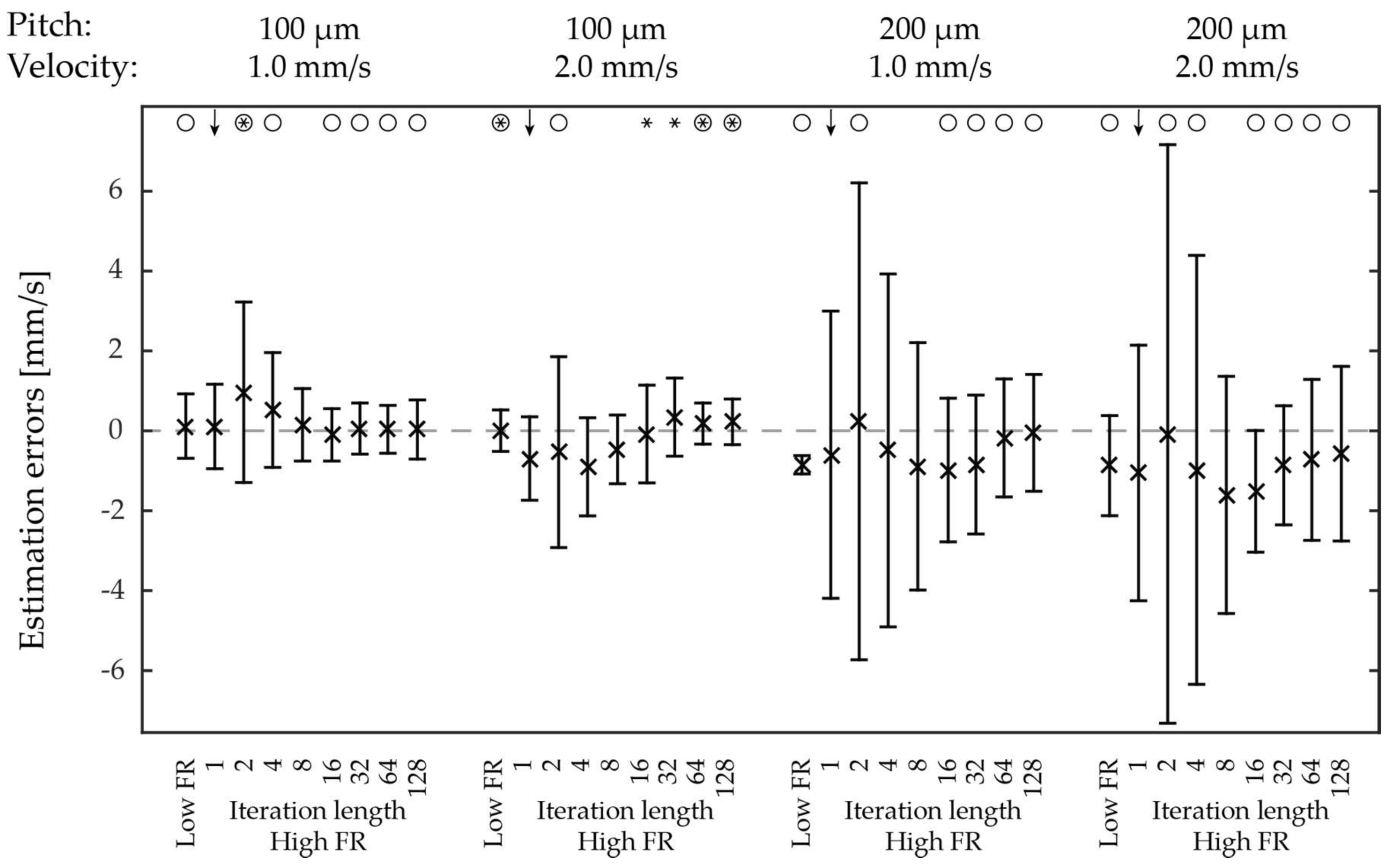
| Pitch | 100 µm | 200 µm | 100 µm | 200 µm | |
| Velocity | 1000 µm/s | 1000 µm/s | 2000 µm/s | 2000 µm/s | |
| Significance | - | a, b | - | - | |
| Low FR | 117 ± 805 | −852 ± 229 | 4 ± 520 | −871 ± 1253 | |
| High FR | k = 1 | 108 ± 1058 | −598 ± 3595 | −691 ± 1044 | −1055 ± 3198 |
| k = 128 | 32 ± 742 | −51 ± 1462 | 225 ± 570 | −572 ± 2184 | |
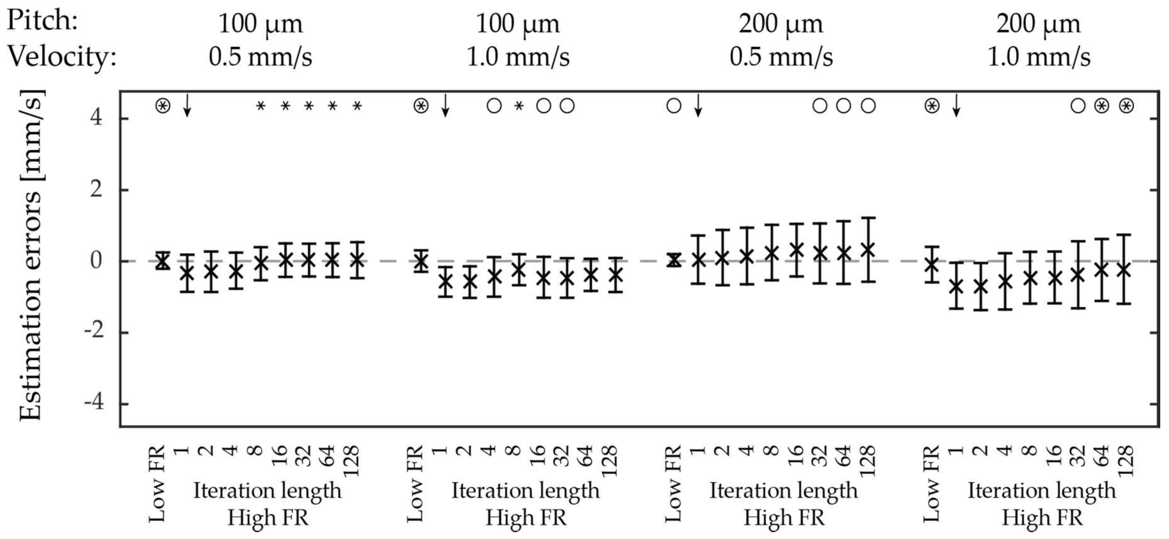
| Pitch | 100 µm | 200 µm | 100 µm | 200 µm | |
| Velocity | 500 µm/s | 500 µm/s | 1000 µm/s | 1000 µm/s | |
| Significance | a, c | a, b | - | a, c | |
| Low FR | 22 ± 228 | 39 ± 167 | 9 ± 302 | −90 ± 497 | |
| High FR | k = 1 | −333 ± 502 | 50 ± 674 | −576 ± 415 | −681 ± 643 |
| k = 128 | 35 ± 504 | 324 ± 896 | −381 ± 475 | −223 ± 967 | |
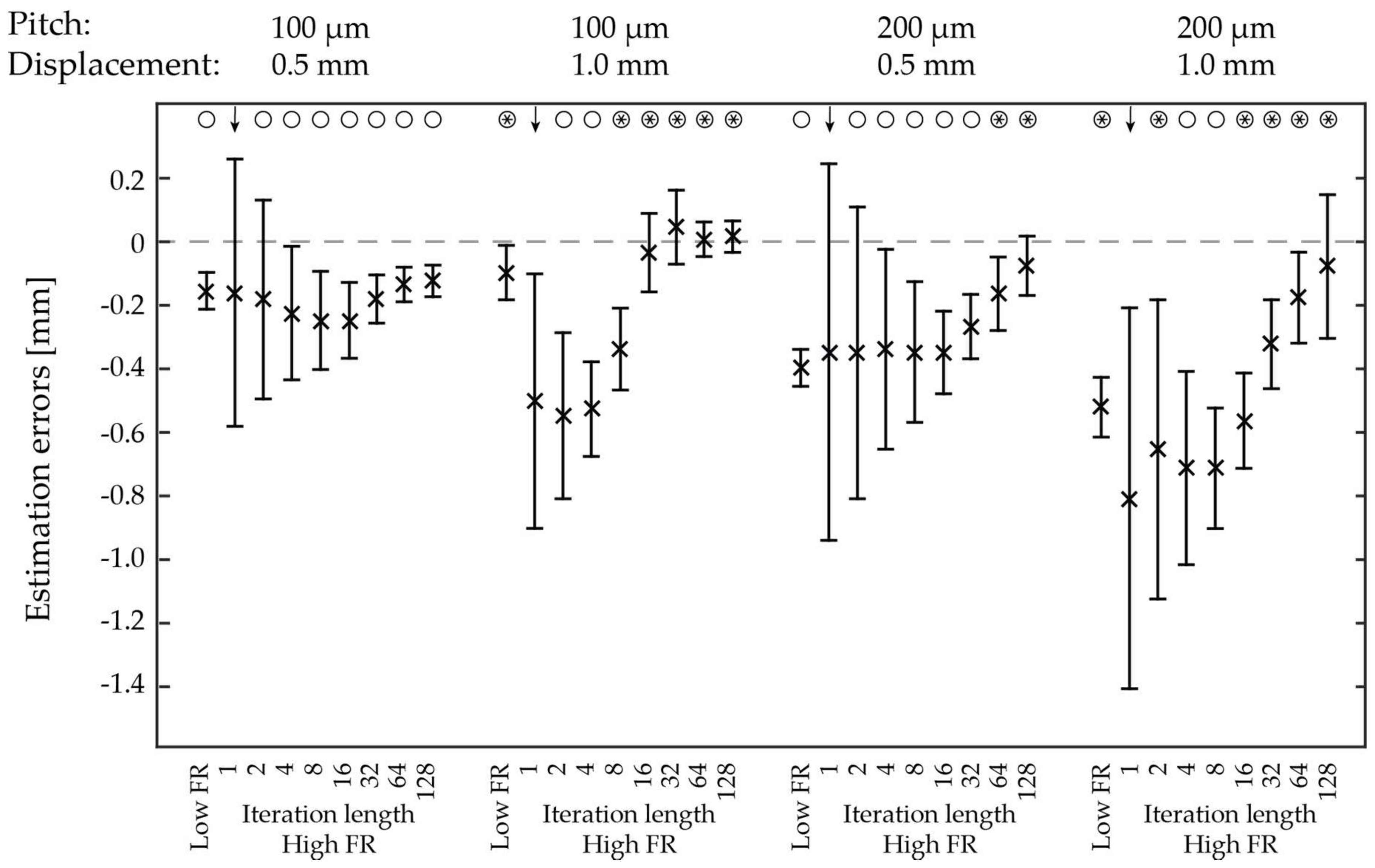
| Pitch | 100 µm | 200 µm | 100 µm | 200 µm | |
| Displacement | 500 µm | 500 µm | 1000 µm | 1000 µm | |
| Significance | - | a, b, c | b, c | a, b, c | |
| Low FR | −154 ± 58 | −397 ± 58 | −97 ± 86 | −521 ± 94 | |
| High FR | k = 1 | −160 ± 421 | −347 ± 592 | −501 ± 400 | −807 ± 599 |
| k = 128 | −123 ± 50 | −75 ± 93 | 16 ± 49 | −78 ± 226 | |
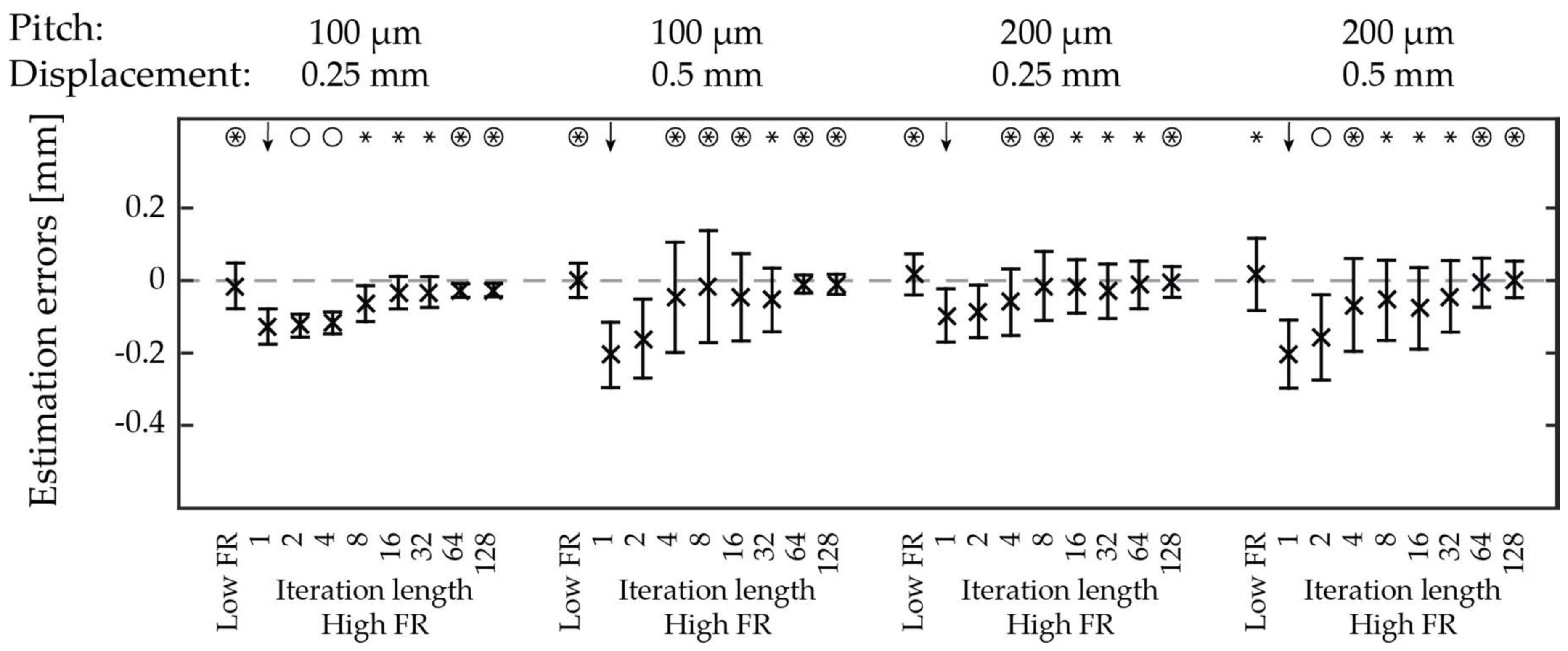
| Pitch | 100 µm | 200 µm | 100 µm | 200 µm | |
| Displacement | 250 µm | 250 µm | 500 µm | 500 µm | |
| Significance | a, c | a, c | a, c | a, c | |
| Low FR | −15 ± 63 | 17 ± 57 | 1 ± 47 | 17 ± 100 | |
| High FR | k = 1 | −127 ± 49 | −96 ± 74 | −206 ± 90 | −203 ± 94 |
| k = 128 | −26 ± 18 | −4 ± 43 | −10 ± 28 | 3 ± 51 | |
© 2018 by the authors. Licensee MDPI, Basel, Switzerland. This article is an open access article distributed under the terms and conditions of the Creative Commons Attribution (CC BY) license (http://creativecommons.org/licenses/by/4.0/).
Share and Cite
Albinsson, J.; Hasegawa, H.; Takahashi, H.; Boni, E.; Ramalli, A.; Rydén Ahlgren, Å.; Cinthio, M. Iterative 2D Tissue Motion Tracking in Ultrafast Ultrasound Imaging. Appl. Sci. 2018, 8, 662. https://0-doi-org.brum.beds.ac.uk/10.3390/app8050662
Albinsson J, Hasegawa H, Takahashi H, Boni E, Ramalli A, Rydén Ahlgren Å, Cinthio M. Iterative 2D Tissue Motion Tracking in Ultrafast Ultrasound Imaging. Applied Sciences. 2018; 8(5):662. https://0-doi-org.brum.beds.ac.uk/10.3390/app8050662
Chicago/Turabian StyleAlbinsson, John, Hideyuki Hasegawa, Hiroki Takahashi, Enrico Boni, Alessandro Ramalli, Åsa Rydén Ahlgren, and Magnus Cinthio. 2018. "Iterative 2D Tissue Motion Tracking in Ultrafast Ultrasound Imaging" Applied Sciences 8, no. 5: 662. https://0-doi-org.brum.beds.ac.uk/10.3390/app8050662