A Novel Image Feature for the Remaining Useful Lifetime Prediction of Bearings Based on Continuous Wavelet Transform and Convolutional Neural Network

Abstract

In data-driven methods for prognostics, the remaining useful lifetime (RUL) is predicted based on the health indicator (HI). The HI detects the condition of equipment or components by monitoring sensor data such as vibration signals. To construct the HI, multiple features are extracted from signals using time domain, frequency domain, and time–frequency domain analyses, and which are then fused. However, the process of selecting and fusing features for the HI is very complex and labor-intensive. We propose a novel time–frequency image feature to construct HI and predict the RUL. To convert the one-dimensional vibration signals to a two-dimensional (2-D) image, the continuous wavelet transform (CWT) extracts the time–frequency image features, i.e., the wavelet power spectrum. Then, the obtained image features are fed into a 2-D convolutional neural network (CNN) to construct the HI. The estimated HI from the proposed model is used for the RUL prediction. The accuracy of the RUL prediction is improved by using the image features. The proposed method compresses the complex process including feature extraction, selection, and fusion into a single algorithm by adopting a deep learning approach. The proposed method is validated using a bearing dataset provided by PRONOSTIA. The results demonstrate that the proposed method is superior to related studies using the same dataset.

1. Introduction

In recent years, interest in prognostics and health management (PHM) has rapidly increased across industry. PHM includes machine maintenance and prognostics, and aims to maximize machine availability and reliability. Unexpected machine breakdown can result increased production downtime and maintenance costs and reduced productivity. Therefore, remaining useful lifetime (RUL) prediction is crucial for determining the condition of machines and establishing a maintenance strategy [1,2,3,4]. Vibration sensors are widely used to monitor the condition of the machine. Therefore, RUL prediction methods using vibration signals are actively studied in the industry and academia.

RUL prediction is divided into two major categories: model-based (i.e., physics-based) methods and data-driven methods. The model-based methods derive mathematical or physical models to estimate the degradation process of the machine. The commonly used models include Markov process, Wiener process, and Gaussian mixture model [3]. These methods rely on the expert’s domain knowledge of the failure mechanism. However, in practice, creating a robust mathematical model is difficult because of the complex and noisy working environments [5]. On the contrary, data-driven methods derive their health indicators (HIs) from measured data, e.g., vibration signals, using signal processing and machine learning techniques. Data-driven methods can be limited when the collected data is insufficient or uncertain. However, if massive data are available, degradation trends can be estimated without physical domain knowledge. Data-driven methods are more flexible and easier to apply to the system than model-based methods. Particularly, with the development of advanced sensors and computing technologies, data-driven prognostics methods have become much more popular in recent years [6]. In this study, we focus on data-driven methods to predict the RUL from vibration signals.

The general framework of data-driven prognostics methods comprises three steps: data acquisition, HI construction, and RUL prediction [7]. The performance of RUL prediction relies on the HI construction step. Therefore, the most important challenge is to extract representative features from the measured signals. A HI that is properly designed by using high-quality features can efficiently monitor the degradation of bearings [8]. Many studies related to feature extraction for prognostics have been conducted [8,9,10]. Time domain and frequency domain analyses are traditional methods for extracting features from vibration signals. Wang et al. [11] extracted 14 time domain features using statistics such as root mean square, mean, variance, and crest factor to denoise the raw signal and capture the degradation trend. Time domain features are suitable for stationary signals. However, they may be sensitive to changes in the signal and could inherit nonlinearity [12]. Frequency domain features can describe additional information that cannot be observed in the time domain because of their superior ability to identify and isolate frequency components [13]. Time–frequency domain features consider both time and frequency domains. Generally, the vibration signal of a bearing is nonstationary and has a weak defect signal within a strong background of noise. Time–frequency analysis is a powerful and effective way to analyze nonstationary and transient vibration signals. Short-time Fourier transform, wavelet transform, wavelet packet decomposition (WPD), and empirical mode decomposition (EMD) have been extensively used to extract features from raw signals [14,15,16,17,18]. The HI is constructed using comprehensive multi-domain feature information, including time domain, frequency domain, and time–frequency domain. Therefore, researchers have proposed suitable HIs by selecting, extracting, and fusing multiple features. Hong et al. [4] extracted time–frequency features using WPD and EMD techniques. Then, they used self-organizing maps (SOM) to construct a HI confidence value (CV). Soualhi et al. [19] analyzed vibration signals using the Hilbert-Huang transform and developed a HI using support vector machine and support vector regression (SVR). Zhao et al. [20] extracted textual features of time-frequency representation and predicted RUL by transforming high-dimensional features into low-dimensional features using principal component analysis and linear discriminant analysis (LDA). Lei et al. [3] proposed the use of the weighted minimum quantization error (WMQE) as a HI, which is a fusion of 10 time domain features, 16 time-frequency domain features, and two features based on trigonometric functions. While most of these studies relied on feature extraction, selection, and fusion techniques to construct the HI, these complex processes are labor-intensive. Additionally, HIs constructed using shallow models (e.g., SVR or LDA) lack prognostics capability and adaptability [6].

To solve these problems, various deep learning techniques (e.g., convolutional neural networks (CNNs), deep belief networks, and recurrent neural networks (RNNs)) have been employed to build advanced HIs for big data. Ren et al. [21] proposed an integrated deep learning approach-based HI by fusing both time and frequency domain features. The method captured high-quality degradation trends of rolling bearings from massive data. Guo et al. [2] extracted 11 time domain features, five frequency domain features, and eight time–frequency domain features. The most sensitive features were selected using monotonicity and correlation metrics. The selected features were fed into an RNN architecture to construct a HI. The RNN-HI has proved to be superior to the SOM-based HI. These studies improved prediction performance using the deep learning approach, but expert knowledge or feature engineering is still required. Therefore, instead of extracting and fusing multi-domain features, researchers have adopted CNN to automatically discover useful features from the raw signal to construct the HI. The CNN was first proposed by LeCun et al. [22] and has led to considerable advancements in image processing and speech recognition. Zhao et al. [5] developed convolutional bi-directional long short-term memory (CBLSTM) networks to predict tool-wear conditions. They extracted local features using the convolutional and pooling layers of the CNN from the raw signal. The features are inputted into long short-term memory (LSTM) neural networks to construct the HI. Eren [23] also directly inputted the raw signal to a one-dimensional (1-D) CNN, which incorporates feature extraction and fault detection into a single algorithm. Although the CNN was originally designed to process two-dimensional (2-D) visual signals, most of the research in the prognostics field has been used to process 1-D vibration signals. To improve the feature extraction of the CNN, another study has been conducted using a 2-D CNN based on the time-window approach after converting multi-sensor signals into a 2-D form [1]. However, limitations still exist in using the raw signal instead of 2-D image data. Generally, the vibrational raw signal contains a large amount of noise and has nonstationary characteristics. Therefore, if the raw signal is used to learn, it can degrade the learning capability of the CNN [24].

To address these issues, we present a novel image feature-based CNN method that adopts the continuous wavelet transform (CWT) for HI construction and RUL prediction. The CWT performs a 2-D wavelet transform of the time–frequency domain to convert the vibration signal into a multi-scale power spectrum image. The power spectrum visually shows that the frequency components have changed over time. In addition, it does not require the analyst to have much experience in fault diagnosis or signal processing [25]. As a result, the CWT is widely used for mechanical fault diagnosis such as bearings and gearboxes [26,27]. Therefore, we adopted the CWT to take the visual advantage of decomposing vibration signals and localizing faults. Wavelet-based feature extraction and CNN application have been studied in machine fault classification. However, in the PHM field, it has become increasingly important to predict the RUL accurately for predictive maintenance, rather than simply diagnosing and classifying faults in a machine or component [24,28,29]. To the best of our knowledge, no research on RUL prediction using deep learning with 2-D image features is found in the literature. Therefore, we propose the image feature-based RUL prediction method. The proposed method can be used for prognosis as well as diagnosis.

Our major contribution is to improve the accuracy of RUL prediction using the HI combined with CWT and CNN (i.e., CWT- and CNN-based HI (CWTCNN-HI)). First, CWT is used to convert a 1-D vibration signal into a 2-D image feature using wavelet power spectrum. The raw signal contains only time domain information, but the transformed image feature is effective for visualizing both time and frequency domain information of the vibration signals. In addition, CWT can effectively isolate non-stationary and transient data such as vibration signals and can detect weak defect signal, even in strong noises [26]. Once the raw signal is converted into an image feature, the image is directly entered into the 2-D CNN architecture. CNN is used as a regression model to estimate the CWTCNN-HI based on training images. The HI quantifies the condition of the machine or component. Since the RUL is predicted by the estimated HI, the accuracy of the prediction model becomes critical. Although CNN requires a large amount of training data and tuning of hyper-parameters, previous studies have shown its superior performance in image analysis [28,29,30]. In addition, CNN automatically discovers useful features through multi-layer convolutional filters. Therefore, the process of extracting, selecting, and fusing multi-domain features can be compressed with a single algorithm. With more training data, prediction performance of the proposed method can be improved. In this study, we use the vibration dataset of bearings provided by PRONOSTIA for RUL prediction [31]. The experimental results demonstrate the superiority of the proposed method compared to related works on the same dataset.

The rest of the paper is organized as follows. Section 2 presents the proposed CWTCNN-HI with brief introductions of CWT and CNN. Section 3 showcases the validation of the proposed method using the PRONOSTIA dataset, and the experimental results are compared to other related research. Finally, in Section 4, we conclude with a discussion and mention future research topics.

2. Time–Frequency Image Feature-Based HI

In this section, we present the deep learning-based HI for RUL prediction. The procedure of the CWTCNN-HI-based method is shown in Figure 1. This method is composed of three stages: image feature extraction, CWTCNN-HI construction, and RUL prediction. In the feature extraction stage, image features are extracted from raw vibration signals using CWT. The image features of the training dataset are utilized to construct deep learning-based HI in the CWTCNN-HI construction stage. The CWTCNN-HI model learns how frequency changes with the machine health condition from training image features. The trained CWTCNN-HI model estimates the HI by inputting the image features of the testing dataset. In the RUL prediction stage, the remaining lifetime is derived by assuming that the failure occurs at the time the predicted HI reaches the threshold. The Gaussian process regression (GPR) algorithm is used to predict HI and future degradation trends based on the estimated HI. Then, to specify the threshold for RUL prediction, the testing datasets are clustered considering the similar degradation trend. Finally, the RUL is predicted by calculating the difference between the time at which the predicted HI reaches the threshold and the current time. More details about each of the stages in the proposed prognostics method are presented as follows.

2.1. Continuous Wavelet Transform (CWT)

The CWT decomposes the signal into a time-scale plane by scaling and shifting the basis wavelet. A mother wavelet, $\psi \in L^2\left(R\right)$, is a function of zero average and finite length, where $L^2\left(R\right)$ is the space of square-integrable complex functions [24,26,28]. The family of time-scale waveforms is obtained by shifting and scaling the mother wavelet:

$${\psi }_{a, b}\left(t\right)={\left|a\right|}^{-\frac{1}{2}}\psi \left(\frac{t-b}{a}\right),$$

(1)

where $a$ is the scale parameter for dilating or contracting the wavelet, and $b$ is the shifting parameter for transitioning the wavelet along the time axis. Thus, we obtain the components of the lower frequency band using a long wavelet. Alternatively, we obtain a component of the high-frequency band using a short wavelet. For the given signal, $x\left(t\right)$, wavelet coefficient $wt\left(a,b\right)$ can be represented as

$$wt\left(a, b\right)={\left|a\right|}^{-\frac{1}{2}}{\int }_{-\infty }^{\infty }x\left(t\right){\psi }^{*}\left(\frac{t-b}{a}\right)dt,$$

(2)

where ${\psi }^{*}$ denotes the complex conjugate of $\psi$. The CWT is useful for obtaining both frequency and spatial information. It is also better for visualizing the frequency components at different time scales and resolutions. The details of the CWT can be found in the work of Daubechies [32].

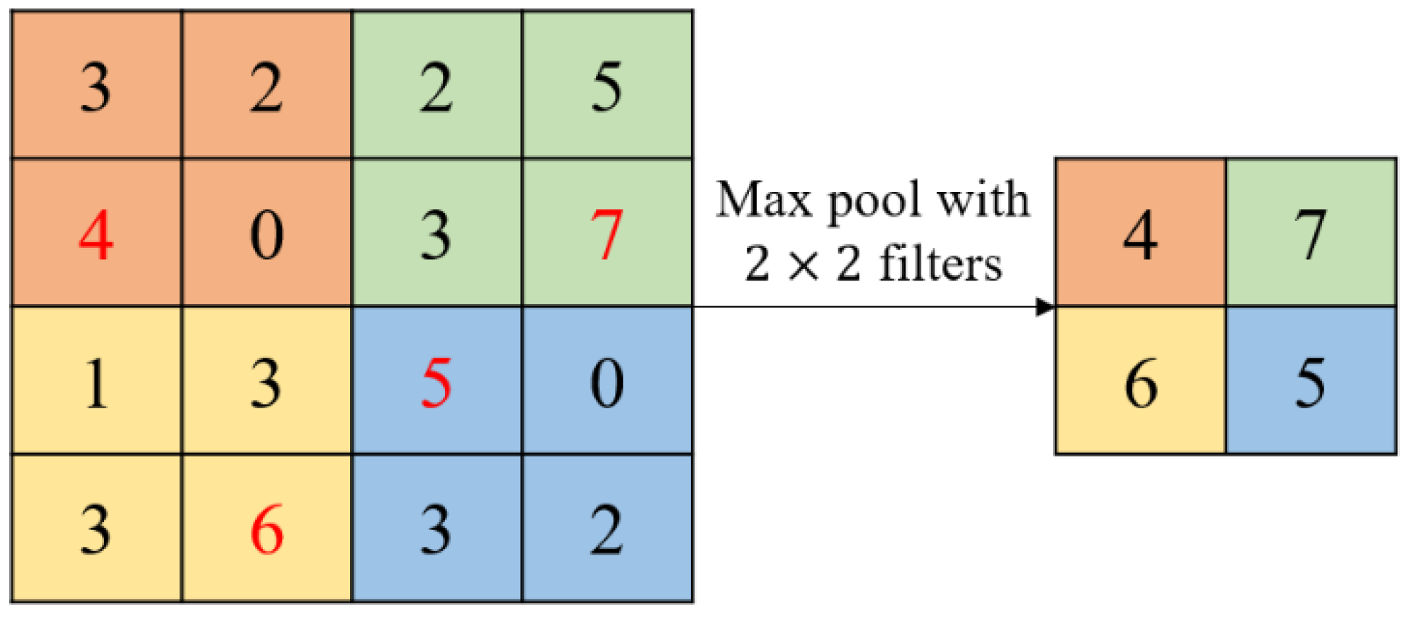
2.2. Basic Theory of CNN

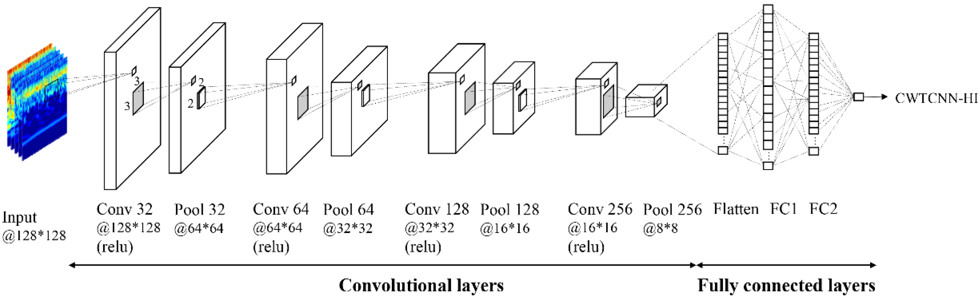
CNN is a deep learning model inspired by the visual cortex of the brain. It is widely used in various fields such as computer vision, natural language processing, and speech recognition because it can analyze an original image directly without complicated preprocessing [24]. A typical CNN comprises three layers: convolutional, subsampling, and fully connected. To extract features from image data, the CNN model alternately stacks the convolutional layer and the subsampling layer, and configures the output layer as a fully connected layer.

The convolutional layers convolve the input from the previous layer with multiple kernels and send it to the activation function to construct a feature map. The output feature map is the convolutional results of the input maps and can be calculated as follows:

$$x_j^l=f\left({\sum }_{i\in M_j}{x}_i^{l-1}\ast k_{ij}^l+b_j^l\right),$$

(3)

where $\ast$ is a convolutional operator, $x_i$ is ith input map, $k$ is a $S\times S$ convolutional kernel, $b_j$ is an additive bias, $M_j$ is a feature map of the convolutional layer, and $l$ is the lth layer in the network. Finally, the convolutional results are passed to the activation function, $f$ [33]. The two most commonly used activation functions (i.e., rectified linear unit (ReLU) and sigmoid function) are defined as follows.

$$ReLU\left(x\right) = max\left(0, x\right)$$

(4)

$$sigmoid\left(x\right)=\frac{1}{1+e^{-x}}$$

(5)

The subsampling layer, located after the convolutional layer, produces low-resolution maps by extracting the most significant local features. The most commonly used max-pooling layer extracts the maximum value from each region, as shown in Figure 2.

All feature maps are combined into a 1-D vector to construct a flatten layer. Then, in the fully connected layer, all neurons of both layers are connected, like a traditional multilayer neural network. The output of the fully connected layer can be expressed by

$$O=f\left({\sum }_{j=1}^d{x}_j^F{w}_j+b\right),$$

(6)

where $O$ is the output value, $x_j^F$ is the jth neuron in the fully connected layer, $w_j$ is the weight corresponding to $O$ and $x_j^F$, $b_i$ is the bias corresponding to $O$, and $f$ is a sigmoid function [28].

2.3. CWTCNN-HI

In this study, we construct a CNN for image-based RUL prediction of the bearing. Wen et al. [30] proposed 12 CNN models based on the classical CNN, LeNet-5, and compared performances. The best CNN structure has shown that it can classify bearing faults with an accuracy of 99.79%. Therefore, we designed the model by referring to the best CNN structure derived from Wen et al. [30]. The structure of the proposed CWTCNN-HI model is shown in Figure 3. To use this model, the input data is prepared by converting the CWT coefficients into a 2-D image. Then, four convolutional layers and four pooling layers are connected alternately for feature extraction. The filter size of the convolutional layer is $3\times 3$, and the filter size of the max pooling layer is $2\times 2$. The channels of the four convolutional layers are 32, 64, 128, and 256. The last layers of the model comprise a flatten layer, two fully connected layers, and one output layer. After the convolutional layers, the 2-D feature map is flattened and connected to the fully connected layer. In the fully connected layers, 2560 and 768 nodes are selected, respectively. Finally, the last fully connected layer and one output neuron are connected to obtain the CWTCNN-HI. The ReLU function is applied to the convolutional and fully connected layers, and the sigmoid function is used on the output layer, normalizing the output HI from 0 to 1. After parameter setting, the model is trained to minimize the loss function

$$LOSS=\frac{1}{T}{\sum }_{t=0}^T{\left(\widehat{Y_t}-Y_t\right)}^2,$$

(7)

where $\widehat{Y_t}$ is a predicted value of the CWTCNN-HI model, $Y_t$ is an actual value at time $t$, and $T$ is a failure time. The Adam optimizer [34] is employed with mini batches to optimize the loss function. The batch normalization is used to accelerate the training process and overcome the overfitting problem of the model. For the experiment, we implemented the Python-based Keras deep learning framework [35], which uses Tensorflow on the back-end to build the CWTCNN-HI model [36]. The parameters used for model training such as optimizer, loss function, and normalization method were chosen by a trial and error method.

3. Experiment and Analysis

In this section, we discuss our enhancements to RUL prediction performance by using the image feature and deep learning approach. Experiments were conducted using the bearing degradation datasets to verify the effectiveness and superiority of the proposed method.

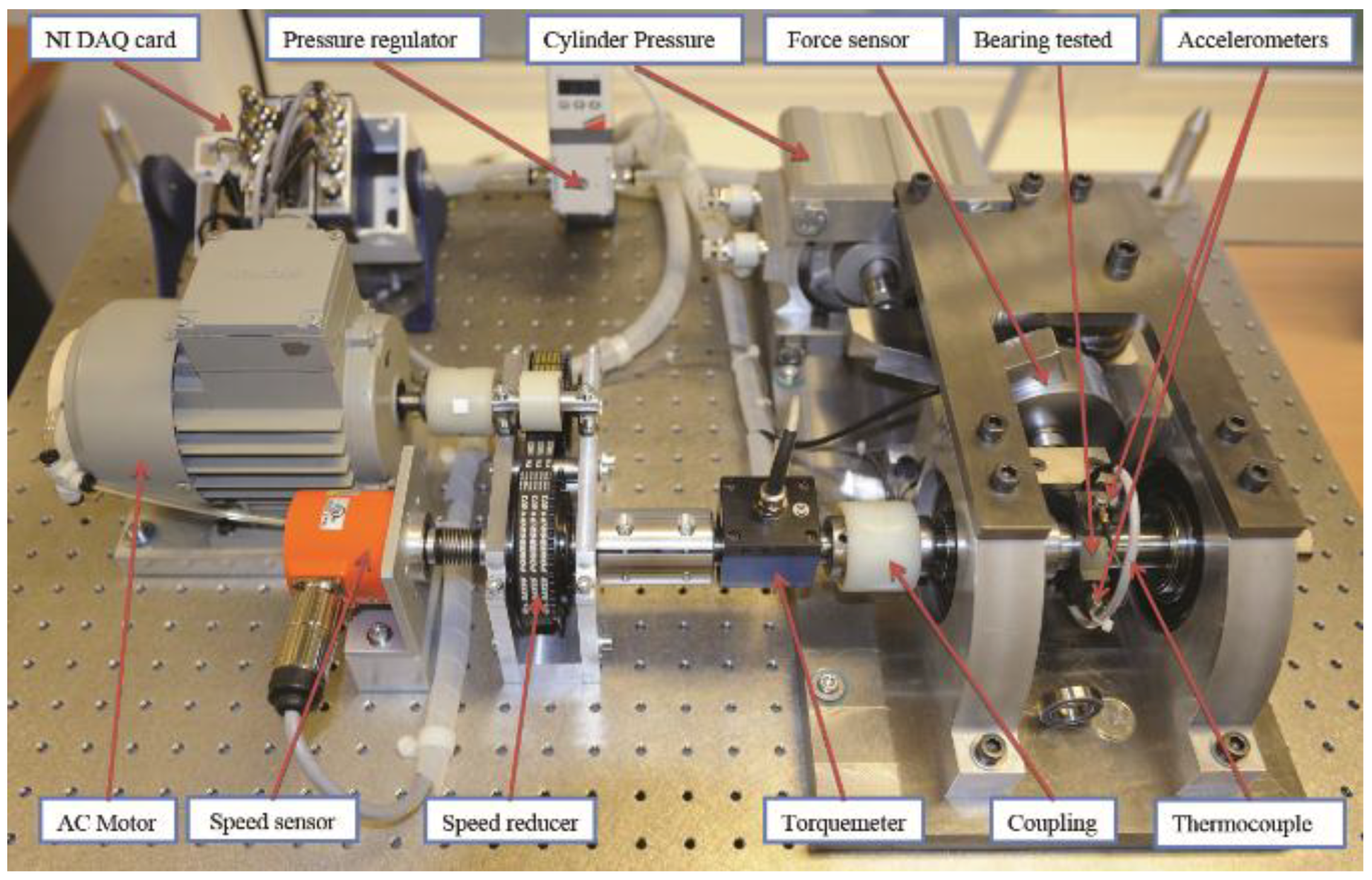
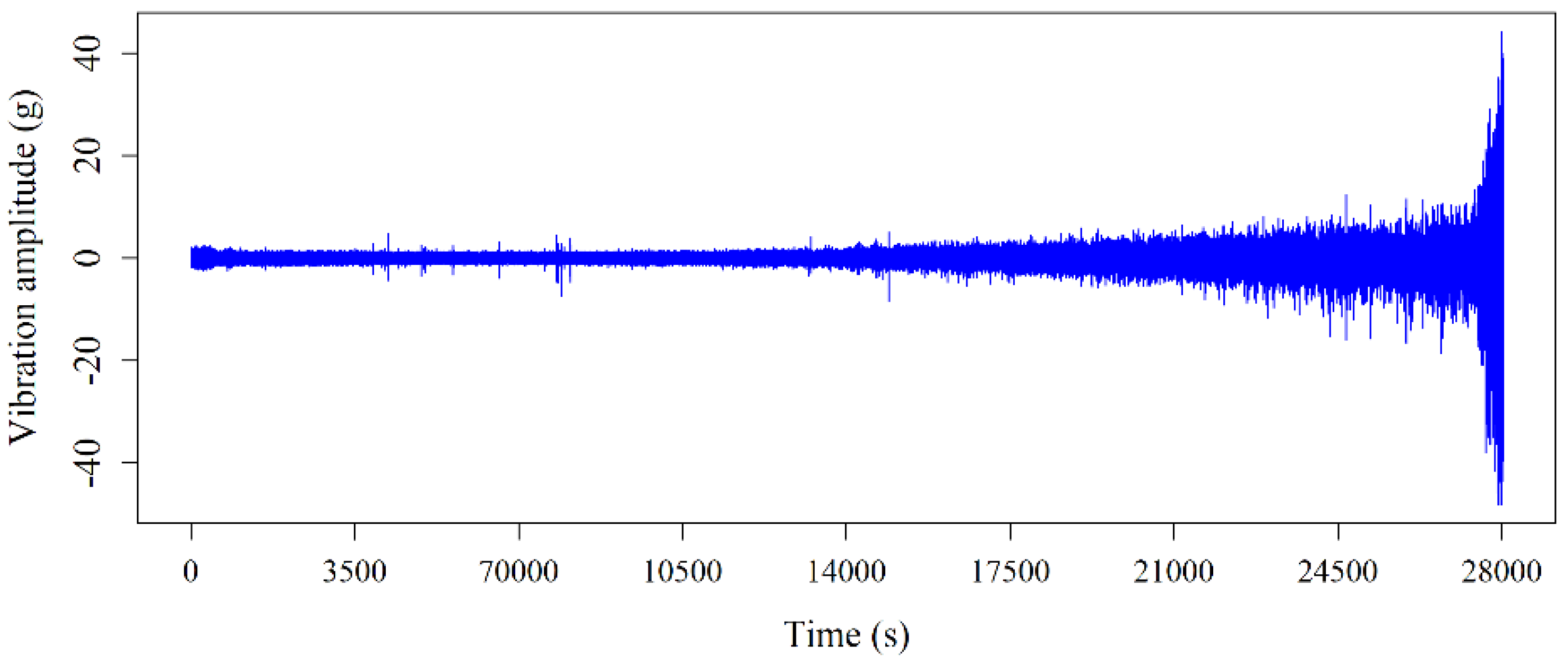
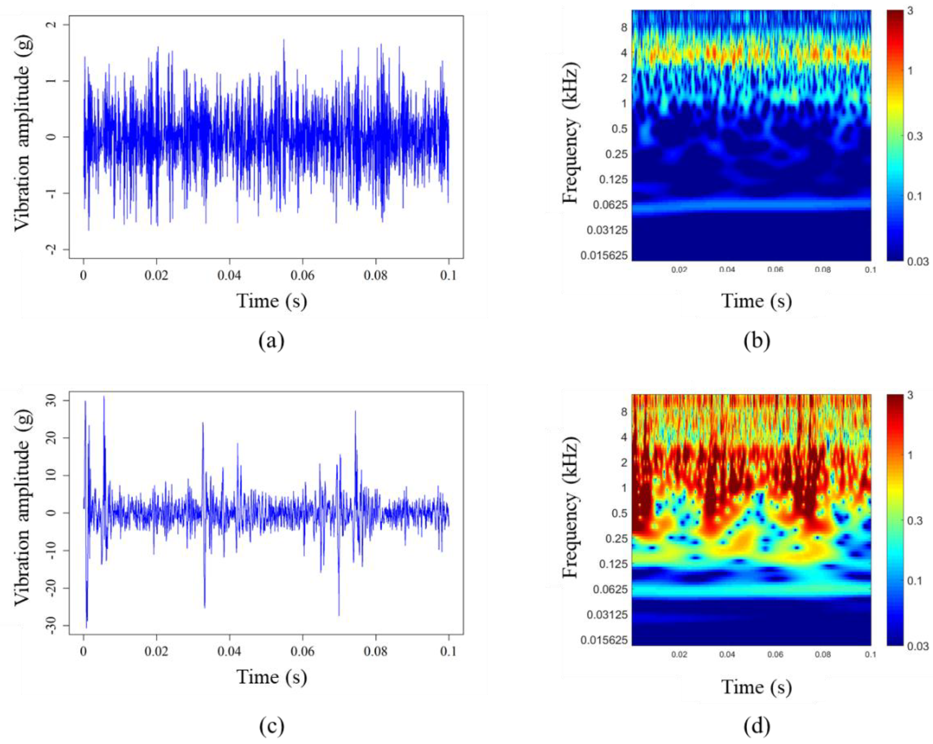
3.1. Experimental System and Vibration Data

The experimental dataset was collected on the PRONOSTIA platform, provided by the FEMTO-ST Institute [31]. This dataset was used in the IEEE PHM 2012 Data Challenge for predicting the RUL of bearings. The PRONOSTIA platform is shown in Figure 4. The experimental platform conducted accelerated degradation tests to collect degradation data of ball bearings until their total failure. The vibration signals were measured by two accelerometers placed on the vertical and horizontal axes. Acceleration measures were sampled every 10 s for a sample period of 0.1 s and a frequency of 25.6 kHz.

In the experiment, 17 bearings were tested under three different operating conditions (i.e., 1800 rpm and 4000 N, 1650 rpm and 4200 N, and 1500 rpm and 5000 N), as shown in

Table 1. Bearing dataset with operational conditions.

Operational Conditions	Speed (rpm)	Load (N)	Training Dataset	Testing Dataset
Condition1	1800	4000	Bearing1_1	Bearing1_3	Bearing1_4	Bearing1_5
			Bearing1_2	Bearing1_6	Bearing1_7
Condition2	1650	4200	Bearing2_1	Bearing2_3	Bearing2_4	Bearing2_5
			Bearing2_2	Bearing2_6	Bearing2_7
Condition3	1500	5000	Bearing3_1	Bearing3_3
			Bearing3_2

. In the three operation groups, there were seven, seven, and three bearings. The first two bearings of each group were used for training the run-to-failure dataset, and the remaining 11 bearings were truncated to predict the RUL. The bearings were naturally degraded without initially assuming a type of failure. Therefore, the degradation patterns of the bearings differed from each other. Any failures of the balls, rings, or cage could occur simultaneously.

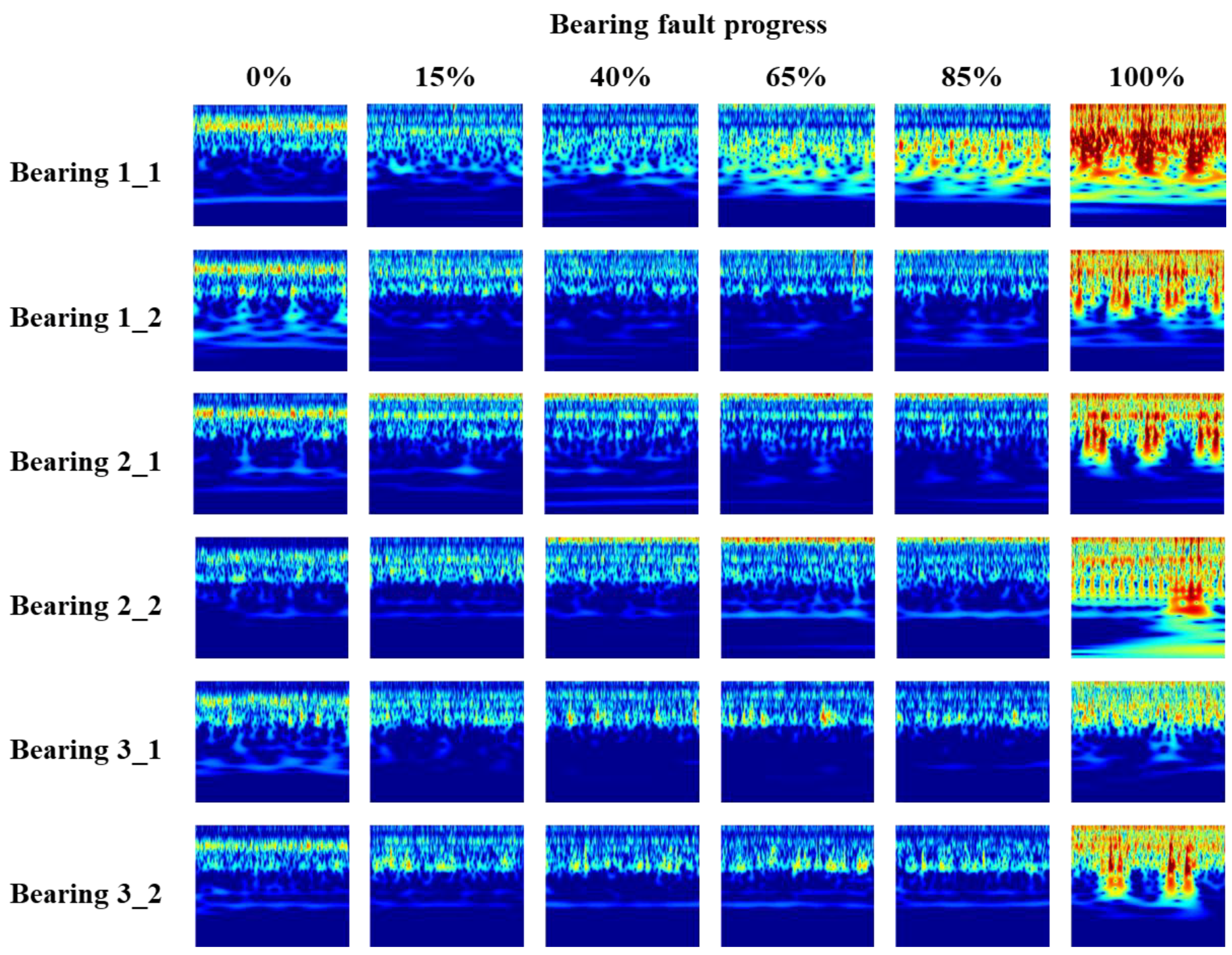
3.2. Extraction of Time—Frequency Image Features

The vibrational raw signal of bearing 1_1, during its whole lifetime, is shown in Figure 5. In the time domain vibration signal, the horizontal and vertical axes represent time and amplitude, respectively. The unit g, representing the acceleration of gravity, is usually used to define the amplitude. Here, 1 g is equivalent to 9.81 $\mathrm{m}/{\mathrm{s}}^2$. The amplitude of the vibration signal increased gradually over time, indicating that the signal had abundant information for diagnostics and bearing prognostics. High-quality features of the vibration signal contain useful information about degradation and effectively filter out unnecessary information. However, the traditional fault diagnosis features, based on frequency domain analysis, did not work efficiently, because the vibration of bearings was nonstationary and nonlinear. Additionally, the frequency resolution was too low for detailed analysis [7].

In this study, we used the Morlet-based CWT to extract image features from the raw vibration signal. The basic principle of determining a wavelet function is to select a shape similar to the vibration signal generated by a mechanical fault. The vibration signals from a failed bearing contain periodic impulses, and the shape of the signal is known to be similar to the Morlet wavelet. In addition, the previous studies have proven superior performance of fault classification using CNN with the Morlet-based CWT [28,29]. Therefore, the Morlet wavelet was chosen in this study.

Figure 6 depicts the raw vibration signal and contour plot of wavelet power spectrum generated by the Morlet-based CWT. The vibration signal sampled for 0.1 s at frequencies of 25.6 kHz has 2560 data points. Figure 6a shows a normal vibration signal and Figure 6c shows a fault vibration signal. When the bearing is in a fault condition, the amplitude of the signal is about −30 g to 30 g, which is larger than in the normal condition. In the wavelet power spectrum, the horizontal axis and vertical axis represent time and frequency, respectively. The color of each point indicates the magnitude of the wavelet coefficients on the time–frequency grid. The red color means that the energy level is high. In Figure 6b, when the bearing is operating in normal condition, the most of the energy is concentrated around 4 kHz. There is no clear periodicity in the energy distribution. On the other hand, Figure 6d shows energy bursts in the frequency range from about 0.25 kHz to over 8 kHz. The impacts occur in the frequency band between 0.25 kHz and 1 kHz at regular interval. When high energy is observed in the low frequency band, it notices that the bearing is heading to the defect [25].

Figure 7 shows image features during the run-to-failure experiment of the training bearings. They show the energy distribution of vibration signals according to the degree of progression of defects in the time-frequency domain. The fault progress is calculated as a percentage of the operation time over the lifetime of the bearing. Therefore, the fault progress of the bearing starts from 0% and gradually increases with the operating time. In this study, we assumed that the bearing fails if the fault progress reaches 100%. In Figure 7, the image features clearly visualize the degradation process in all training bearings. Especially, as the fault progress approaches 100%, high energy is observed, and the impacts occur at regular interval in the low frequency band.

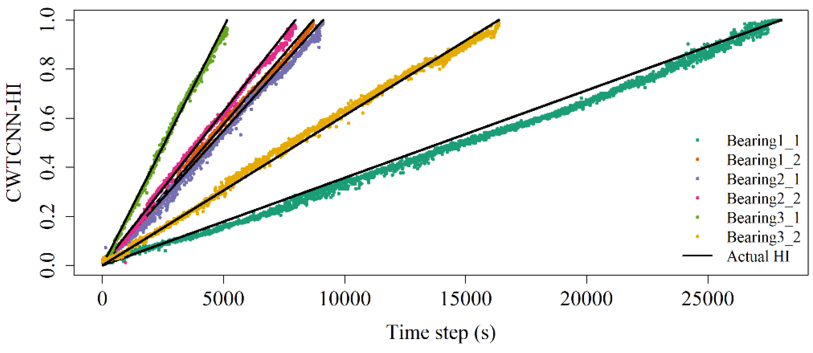
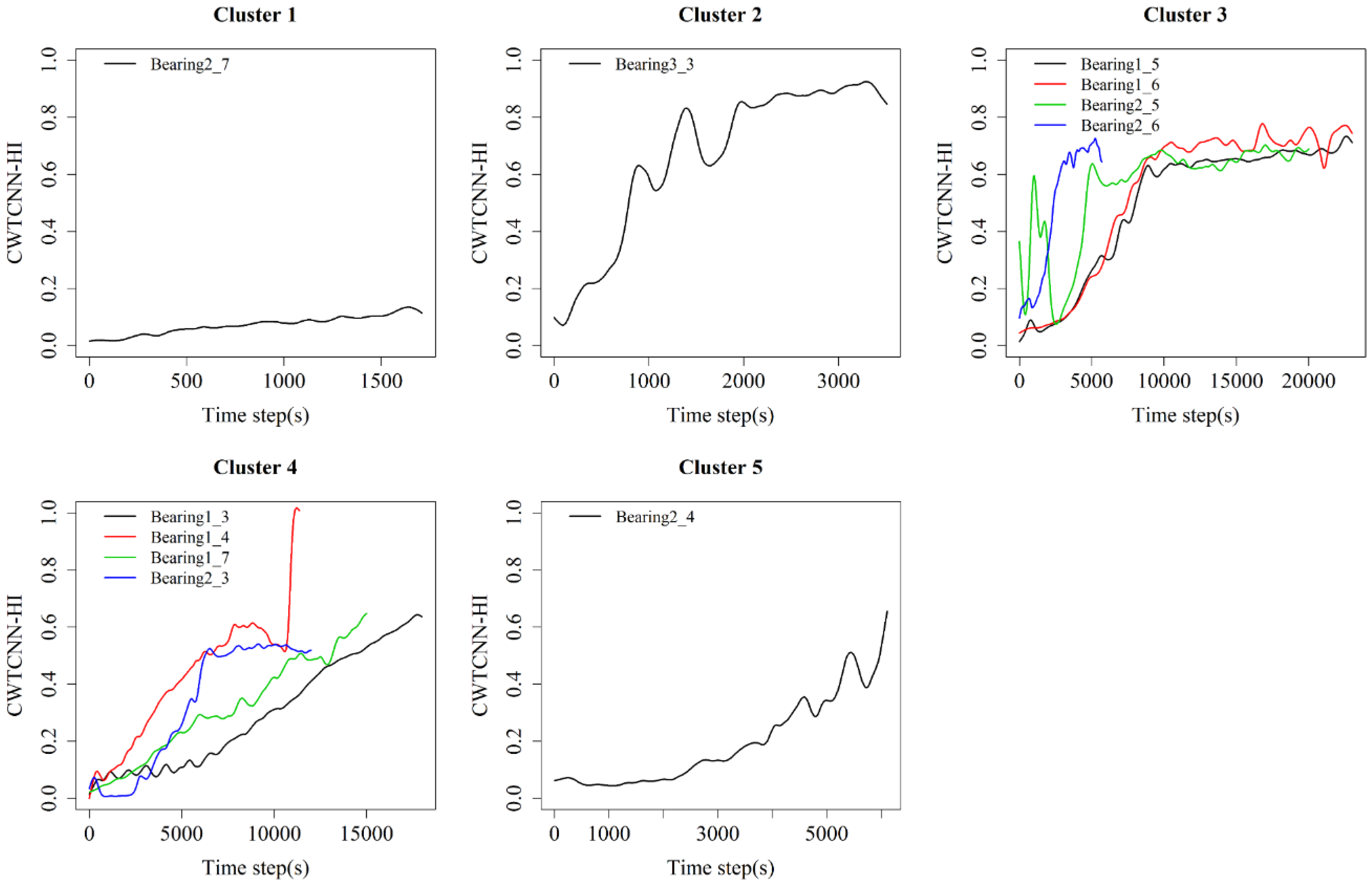
3.3. CWTCNN-HI Construction

The proposed model comprised a training step and a testing step. During the training step, six bearings were used as a training set to construct the model for CWTCNN-HI estimation. The training bearings are the same as those used in the IEEE PHM 2012 Data Challenge. The training set is represented by $D_{train}={\left\{x_t, y_t\right\}}_{t=1}^T$, where $x_t\in R^{N\times N}$ is $N\times N$ image features extracted at time $t$, and $y_t\in \left[0,1\right]$ is a label indicating degradation percentage of bearings at time $t$. In this study, the size of the input image feature is $128\times 128$. The degradation percentage is calculated as $y_t=t/T$, where $t$ is the operation time, and $T$ is the failure time (i.e., lifetime). For example, if the failure time of a bearing is 28,000 s, the degradation percentage, $y_t$, is 0.5 at 14,000 s. The testing set is denoted by $D_{test}={\left\{x_t\right\}}_{t=1}^T$, where $x_t$ is also $N\times N$ image features extracted from the testing dataset. In the testing step, the image features of the testing dataset were entered into the trained model to obtain the CWTCNN-HI.

In the training step, we used approximately 7500 image features extracted from the six training bearings to construct the CWTCNN-HI model. The training results are shown in Figure 8. The horizontal axis represents the operating time while vertical axis represents the CWTCNN-HI value. The estimated HI is marked as the colored points in the figure and the black line represents the actual HI of the training bearings. The operating time to failure of the training bearings varies from 1 h to 7 h. The estimated HI of bearing 1_1 is slightly different from the actual HI. On the other hand, the estimated HI of the other five bearings generally have a similar pattern to the actual HI. Some training errors are acceptable because most estimations and actual values tend to match each other. This implies that the CWT-based image features can extract high-quality information about the state of the bearing. Thus, CNN is an effective method to estimate the degradation of bearings by analyzing images.

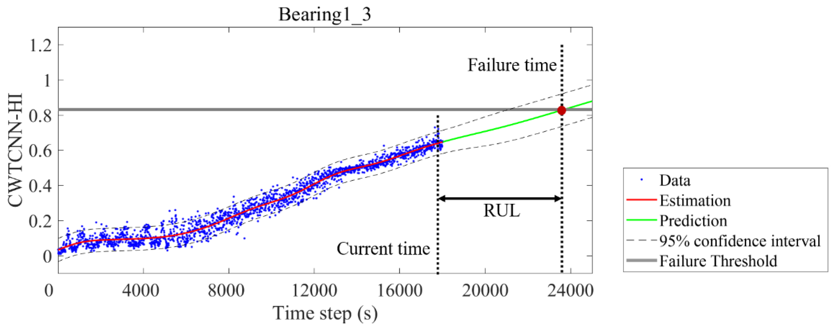
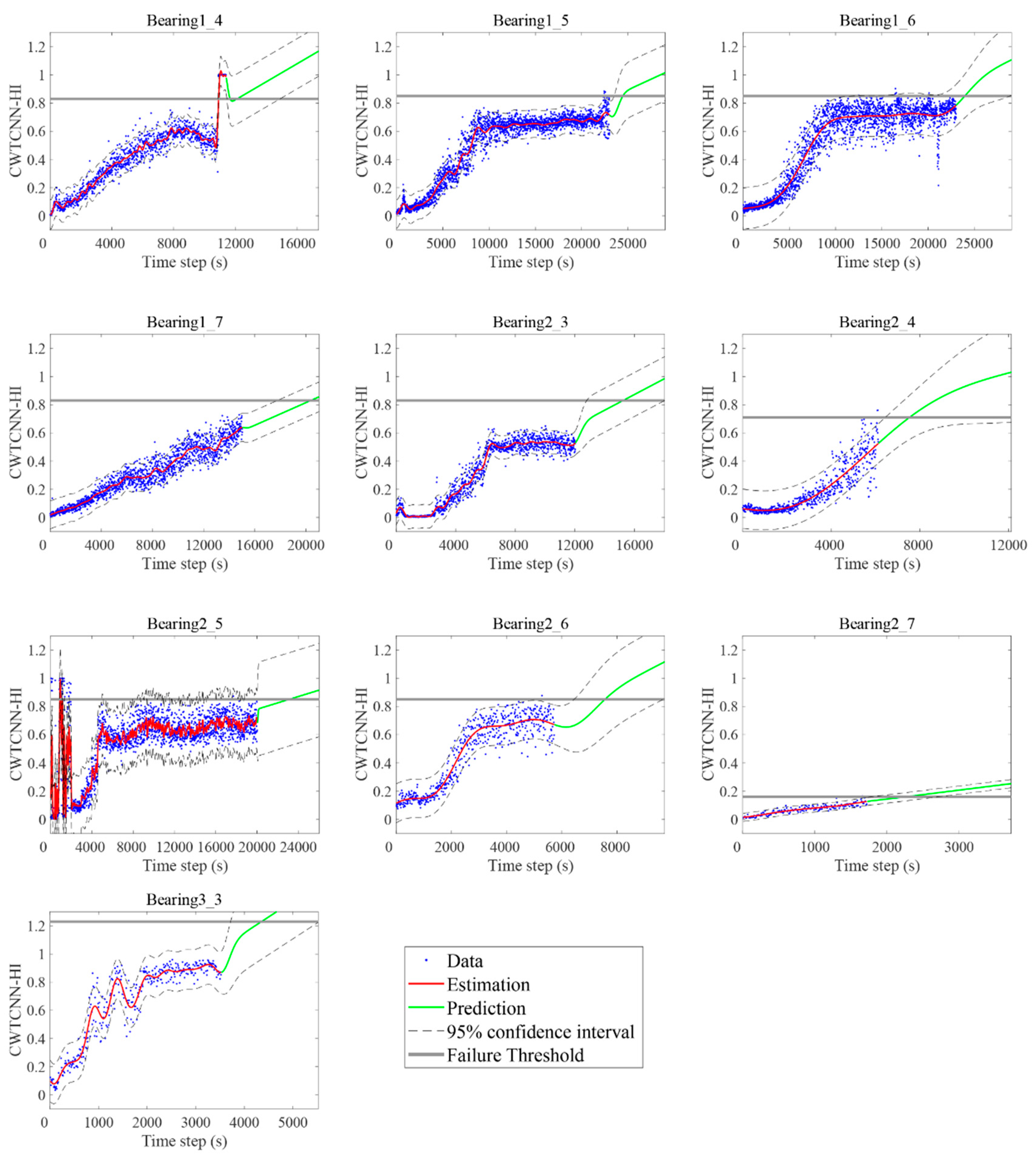
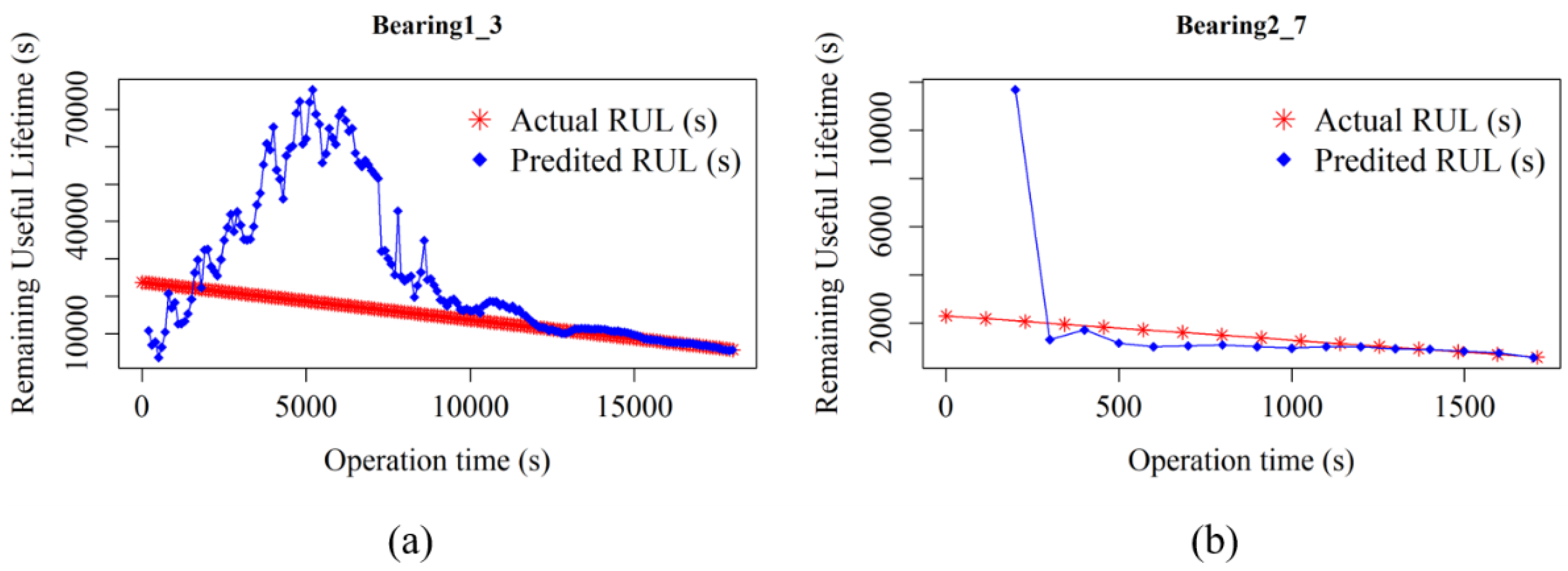
3.4. RUL Prediction Results

Once the CWTCNN-HI was obtained, a GPR algorithm was used to predict the RUL of the test bearings. The GPR is a kernel-based machine learning technique that can conveniently specify high dimensional and flexible nonlinear regression [4]. In this study, we assumed that the mean and covariance functions were zero and a linear function, respectively. Hyper-parameters for the covariance function are optimized by maximizing the log-likelihood function. The GPR model predicts future CWTCNN-HI by estimated CWTCNN-HI up to current time.

The estimated and predicted CWTCNN-HIs of bearing1_3, one of the testing datasets, are shown in Figure 9. The obtained CWTCNN-HI up to the current time is indicated by a dot. The solid lines represent the estimated and predicted CWTCNN-HIs before and after the current time obtained by using the GPR model, respectively. The dotted lines are the 95 % confidence interval. The figure shows that the health condition of the bearing gradually degrades over time with the increase of HI. The RUL is calculated as the difference between the time at which the predicted HI reaches the threshold and the current time. The RUL prediction results can be affected by the number of samples in the training dataset. The large number of samples in the training data improves the accuracy of the estimated CWTCNN-HI. In addition, as the variance of the predicted CWTCNN-HI decreases, the confidence intervals become narrowed and RUL prediction is more reliable.

The RUL prediction results of the other ten testing datasets are shown in Figure 10. Most testing bearings clearly show different degradation patterns, owing to different operating conditions and failure types. For example, bearing1_5 and bearing1_6 rapidly degraded in their early stage and gradually degraded after a certain period. Alternatively, bearing1_7 shows a constantly degrading pattern, like bearing1_3.

In this study, the clustering-based failure threshold was adopted to accurately predict the RUL of testing bearings. The failure threshold can be provided by an application expert or obtained experimentally. In addition, the different thresholds are applied depending on the operating conditions and characteristics of the bearings [4,37]. The bearings with similar operating condition and failure mode exhibit a similar shape of degradation pattern. In this regard, we used the K-means clustering algorithm to cluster testing bearings with similar degradation trends and applied the same threshold for each cluster. The thresholds were chosen empirically to increase the accuracy of the RUL prediction. To determine the number of clusters in the K-means clustering algorithm, the Dunn index [38] was used to evaluate the clustering performance. The Dunn index is calculated as the ratio of the minimum distance between two objects in different clusters to the maximum distance between two objects in the same cluster as follows:

$$D=\frac{mi{n}_{1\le i<j\le n}d\left(i, j\right)}{ma{x}_{1\le k\le n}d\text{'}\left(k\right)},$$

(8)

where $n$ is the number of clusters, $d\left(i,j\right)$ is the distance between the ith cluster and jth cluster, and $d\text{'}\left(k\right)$ is the intra-cluster distance. A high index value means that the objects are well clustered. Based on the Dunn indexes for different number of clusters, as shown in Figure 11, the testing bearings were grouped into five different clusters.

Figure 12 represents the result of clustering. Clusters 3 and 4 include four testing bearings. The remaining three bearings with different degradation trends constitute three clusters. For example, the bearing in cluster 1 shows the pattern of slow and steady degradation. On the other hand, the bearings of cluster 3 show a pattern of rapid initial degradation. The degradation patterns of the bearings vary depending on operational conditions and failure types. Therefore, the clustering-based failure threshold improves RUL prediction performance by applying different threshold to bearings. For each cluster, the failure threshold is set to 0.16, 1.23, 0.85, 0.83, and 0.71, respectively. If new bearings are tested, the RUL can be predicted using the threshold of the cluster with a similar degradation pattern.

Figure 13 shows the comparison of the actual RUL and the predicted RUL of the two samples of bearings. In Figure 13a, the predicted RUL of the initial and middle deterioration states is significantly different from the actual RUL. The estimated HI of bearing 1_3 is fluctuated at the beginning of the operation, and inconsistencies occur in the initial and middle states. However, the predicted RUL is very close to the actual RUL when the bearing operating time exceeds 3 h. Figure 13b shows a slight discrepancy in the initial state, but the overall trend of the estimated RUL follows the change in the actual RUL. In both bearings, the expected RUL of the final state closely matches the actual RUL, even though the operating times are different from each other.

3.5. Comparing Related Works

In this study, we measured the RUL prediction accuracy of testing bearings to evaluate the proposed method and compare with related studies. As a performance evaluation measurement of the RUL prediction, a score metric, mean, and standard deviation (SD) of the percent error were applied. These metrics were used for the IEEE PHM 2012 Prognostic Challenge [31]. The percent error on the ith bearing is defined as follows:

$$E{r}_i=100\times \frac{ActRU{L}_i-{\widehat{RUL}}_i}{ActRU{L}_i},$$

(9)

where $ActRU{L}_i$ and ${\widehat{RUL}}_i$ are, respectively, the actual RUL and the predicted RUL of the ith testing bearing. Underestimates and overestimates of the RUL were considered in different manners by the following scoring function.

$$A_i=\{\begin{array}{c}exp\left(-\ln \left(0.5\right)·\left(E{r}_i/5\right)\right) if E{r}_i\le 0\\ exp\left(+\ln \left(0.5\right)·\left(E{r}_i/20\right)\right) if E{r}_i>0\end{array}$$

(10)

The score $A_i$ is 1 when the percent error is 0. As the percent error increases, the score decreases. If the failure is predicted later than the actual occurrence (i.e., cases in which $E{r}_i\le 0$), the score is cut more than the earlier predictions. The average score of the RUL prediction for all testing bearings is defined as follows.

$$Score=\frac{1}{11}{\displaystyle \sum }_{i=1}^{11}{A}_i$$

(11)

To verify the superiority of the proposed method, we compared the prediction result with the other four similar studies that predicted bearing RULs using the same dataset.

Table 2. Performance comparisons of the proposed method with related research on the PRONOSTIA dataset.

Testing Dataset	Current Time (s)	Actual RUL (s)	Predicted RUL (s)	Er (%)
				Sutrisno et al. [39]	Hong et al. [4]	Lei et al. [3]	Guo et al. [2]	Proposed Method
Bearing1_3	18,010	5730	5670	37	−1.04	−0.35	43.28	1.05
Bearing1_4	11,380	339	270	80	−20.94	5.60	67.55	20.35
Bearing1_5	23,010	1610	1430	9	−278.26	100.00	−22.98	11.18
Bearing1_6	23,010	1460	950	−5	19.18	28.08	21.23	34.93
Bearing1_7	15,010	7570	5360	−2	−7.13	−19.55	17.83	29.19
Bearing2_3	12,010	7530	3220	64	10.49	−20.19	37.84	57.24
Bearing2_4	6110	1390	1410	10	51.80	8.63	−19.42	−1.44
Bearing2_5	20,010	3090	3110	−440	28.80	23.30	54.37	−0.65
Bearing2_6	5710	1290	1840	49	−20.93	58.91	−13.95	−42.64
Bearing2_7	1710	580	530	−317	44.83	5.17	−55.17	8.62
Bearing3_3	3510	820	830	90	−3.66	40.24	3.66	−1.22
Mean				100.27	44.28	28.18	32.48	18.96
SD				173.28	90.29	35.41	37.57	25.59
Score				0.31	0.36	0.43	0.26	0.57

represents the RUL prediction results of our related studies and proposed method. For each testing bearing, the actual RUL and predicted RUL of the proposed method are displayed in columns 3 and 4, respectively. The percent errors of the proposed method are shown in the final column, and the four comparative studies are shown in columns 5 through 8. The mean and SD of the percent errors and the score metric are displayed in the last three rows. The first similar study was published by Sutrisno et al. [39], the winner of the IEEE PHM 2012 Prognostic Challenge. This study predicts the RUL using frequency analysis-based anomaly detection, degradation feature extrapolation, and survival time ratios. However, the method has the disadvantage of defining the anomaly detection time point based on subjective criteria used to calculate the bearing survival time ratios. The means as well as the deviations of the percent errors are large in the table. The second study was published by Hong et al. [4] using the same bearing dataset. They used wavelet packet-EMD for feature extraction and SOM for constructing the HI (i.e., CV). The method shows improved errors over previous studies, but requires the extraction of approximately one hundred features to estimate bearing performance. The third study, published by Lei et al. [3], proposed a new HI (i.e., WMQE) to predict the RUL of bearings. WMQE was constructed by fusing a select few weighted features based on correlation clustering among the 28 features extracted from the bearings. The study showed the best performance among existing studies. The most recent similar study is an RNN-based RUL prediction method published by Guo et al. [2]. The proposed method was also constructed by selecting and fusing multiple features extracted from the time, frequency, and time–frequency domains. To improve the accuracy of RUL prediction, a deep learning approach was adopted. This method demonstrated its superiority over SOM-based HIs. However, it obtained higher percent errors and lower scores than Lei et al. [3].

The proposed method shows overall low percent errors and low deviation, indicating that the model worked accurately and reliably on every tested bearing. The score obtained in the study was 0.57, which is the highest among comparative studies. Compared to similar studies, the proposed method performs better by using only image features instead of complicated extractions, selections, and fusions of multiple numerical features to construct a HI. Additionally, the degradation trends of the bearing show different patterns due to operational conditions and the simultaneous occurrence of various fault types. In this study, we enhanced the RUL prediction accuracy by defining the clustering-based failure threshold, considering a variety of degradation trends, such as accelerated early degradation and monotonic degradation.

4. Conclusions

In this study, we presented a novel image feature for the RUL prediction based on the CWTCNN-HI. In the proposed method, the vibration signal was converted into the 2-D image feature using CWT instead of using the raw vibration signal or extracting multiple statistical features. The image features of the wavelet power spectrum clearly visualize the degradation process of the bearing. 2-D CNN analyzed the image by including information in both the time and frequency domains. It extracted features from the image and constructed the HI without prior knowledge of feature engineering and signal processing. The CNN model was used as a regression model to estimate the HI between 0 and 1. The estimated CWTCNN-HI was used for the RUL prediction. Since the failure type of the bearings is not defined, the bearings with similar degradation patterns are clustered to set the threshold and predict the RUL. This study has experimentally proved that the image feature can estimate the HI reflecting the condition of the bearings and improve the prediction performance of the RUL. Experiments were conducted on the popular PRONOSTIA bearing dataset to validate the effectiveness of the proposed method. As a result, CWTCNN-HI obtained the highest score and the lowest error among the comparative studies. The CNN model automatically extracted, selected, and fused features that reduce the prediction error of the HI from the image features. Therefore, the result demonstrates that using the CWT-based image features and the CNN model is accurate and effective in the RUL prediction.

However, there are still some limitations in the proposed method. In this study, the threshold for each cluster of bearings was defined empirically. In future studies, thresholds will be defined more systematically and mathematically based on the large amounts of training data. In addition, the RUL will be determined by interaction between bearings and the other components in the system. By doing so, we will improve the reliability of the HI by reflecting the correlation between bearings and other parts in the future. The HI based on multisensory signals will also be studied by considering temperature and vibration sensor data.

References

1. Li, X.; Ding, Q.; Sun, J.-Q. Remaining useful life estimation in prognostics using deep convolution neural networks. Reliab. Eng. Syst. Saf. 2018, 172, 1–11. [Google Scholar] [CrossRef]
2. Guo, L.; Li, N.; Jia, F.; Lei, Y.; Lin, J. A recurrent neural network based health indicator for remaining useful life prediction of bearings. Neurocomputing 2017, 240, 98–109. [Google Scholar] [CrossRef]
3. Lei, Y.; Li, N.; Gontarz, S.; Lin, J.; Radkowski, S.; Dybala, J. A model-based method for remaining useful life prediction of machinery. IEEE Trans. Reliab. 2016, 65, 1314–1326. [Google Scholar] [CrossRef]
4. Hong, S.; Zhou, Z.; Zio, E.; Hong, K. Condition assessment for the performance degradation of bearing based on a combinatorial feature extraction method. Digit. Signal Process. 2014, 27, 159–166. [Google Scholar] [CrossRef]
5. Zhao, R.; Yan, R.; Wang, J.; Mao, K. Learning to monitor machine health with convolutional bi-directional LSTM networks. Sensors 2017, 17, 273. [Google Scholar] [CrossRef] [PubMed]
6. Zhao, G.; Zhang, G.; Liu, Y.; Zhang, B.; Hu, C. Lithium-ion battery remaining useful life prediction with deep belief network and relevance vector machine. In Proceedings of the 2017 IEEE International Conference on Prognostics and Health Management (ICPHM), Dallas, TX, USA, 19–21 June 2017; pp. 7–13. [Google Scholar]
7. Lei, Y.; Li, N.; Guo, L.; Li, N.; Yan, T.; Lin, J. Machinery health prognostics: A systematic review from data acquisition to RUL prediction. Mech. Syst. Signal Process. 2018, 104, 799–834. [Google Scholar] [CrossRef]
8. Zhang, Y.; Tang, B.; Han, Y.; Deng, L. Bearing performance degradation assessment based on time-frequency code features and SOM network. Meas. Sci. Technol. 2017, 28, 045601. [Google Scholar] [CrossRef]
9. Wang, B.; Lei, Y.; Li, N.; Lin, J. An improved fusion prognostics method for remaining useful life prediction of bearings. In Proceedings of the 2017 IEEE International Conference on Prognostics and Health Management (ICPHM), Dallas, TX, USA, 19–21 June 2017; pp. 18–24. [Google Scholar]
10. Zhang, B.; Zhang, L.; Xu, J. Degradation feature selection for remaining useful life prediction of rolling element bearings. Qual. Reliab. Eng. Int. 2016, 32, 547–554. [Google Scholar] [CrossRef]
11. Wang, Y.; Peng, Y.; Zi, Y.; Jin, X.; Tsui, K.-L. A two-stage data-driven-based prognostic approach for bearing degradation problem. IEEE Trans. Ind. Inform. 2016, 12, 924–932. [Google Scholar] [CrossRef]
12. Javed, K.; Gouriveau, R.; Zerhouni, N.; Nectoux, P. Enabling health monitoring approach based on vibration data for accurate prognostics. IEEE Trans. Ind. Electron. 2015, 62, 647–656. [Google Scholar] [CrossRef] [Green Version]
13. Yan, W.; Qiu, H.; Iyer, N. Feature extraction for bearing prognostics and health management (PHM)—A Survey. Geofluids 2008, 11, 343–348. [Google Scholar]
14. Kankar, P.K.; Sharma, S.C.; Harsha, S.P. Fault diagnosis of ball bearings using continuous wavelet transform. Appl. Soft Comput. 2011, 11, 2300–2312. [Google Scholar] [CrossRef]
15. Ocak, H.; Loparo, K.A.; Discenzo, F.M. Online tracking of bearing wear using wavelet packet decomposition and probabilistic modeling: A method for bearing prognostics. J. Sound Vib. 2007, 302, 951–961. [Google Scholar] [CrossRef]
16. Wen, C.; Zhou, C. The feature extraction of rolling bearing fault based on wavelet packet—Empirical mode decomposition and kurtosis rule. In Emerging Technologies for Information Systems, Computing, and Management; Wong, W.E., Ma, T., Eds.; Springer: New York, NY, USA, 2013; pp. 579–586. ISBN 978-1-4614-7010-6. [Google Scholar]
17. Loutas, T.H.; Roulias, D.; Georgoulas, G. Remaining useful life estimation in rolling bearings utilizing data-driven probabilistic e-support vectors regression. IEEE Trans. Reliab. 2013, 62, 821–832. [Google Scholar] [CrossRef]
18. Lei, Y.; Lin, J.; He, Z.; Zuo, M.J. A review on empirical mode decomposition in fault diagnosis of rotating machinery. Mech. Syst. Signal Process. 2013, 35, 108–126. [Google Scholar] [CrossRef]
19. Soualhi, A.; Medjaher, K.; Zerhouni, N. Bearing health monitoring based on Hilbert-Huang transform, support vector machine, and regression. IEEE Trans. Instrum. Meas. 2015, 64, 52–62. [Google Scholar] [CrossRef]
20. Zhao, M.; Tang, B.; Tan, Q. Bearing remaining useful life estimation based on time-frequency representation and supervised dimensionality reduction. Measurement 2016, 86, 41–55. [Google Scholar] [CrossRef]
21. Ren, L.; Cui, J.; Sun, Y.; Cheng, X. Multi-bearing remaining useful life collaborative prediction: A deep learning approach. Measurement 2017, 43, 248–256. [Google Scholar] [CrossRef]
22. LeCun, Y.; Boser, B.E.; Denker, J.S.; Henderson, D.; Howard, R.E.; Hubbard, W.E.; Jackel, L.D. Handwritten digit recognition with a back-propagation network. In Advances in Neural Information Processing Systems; Morgan Kaufmann Publishers Inc.: San Francisco, CA, USA, 1990; pp. 396–404. [Google Scholar]
23. Eren, L. Bearing fault detection by one-dimensional convolutional neural networks. Math. Probl. Eng. 2017, 2017, 8617315. [Google Scholar] [CrossRef]
24. Wang, J.; Zhuang, J.; Duan, L.; Cheng, W. A multi-scale convolution neural network for featureless fault diagnosis. In Proceedings of the 2016 International Symposium on Flexible Automation (ISFA), Cleveland, OH, USA, 1–3 August 2016; pp. 65–70. [Google Scholar]
25. Tyagi, S.; Panigrahi, S.K. A simple continuous wavelet transform method for detection of rolling element bearing faults and its comparison with envelope detection. Int. J. Sci. Res. 2017, 6, 1033–1040. [Google Scholar] [CrossRef]
26. Zheng, H.; Li, Z.; Chen, X. Gear fault diagnosis based on continuous wavelet transform. Mech. Syst. Signal Process. 2002, 16, 447–457. [Google Scholar] [CrossRef]
27. Peng, Z.K.; Chu, F.L. Application of the wavelet transform in machine condition monitoring and fault diagnostics: A review with bibliography. Mech. Syst. Signal Process. 2004, 18, 199–221. [Google Scholar] [CrossRef]
28. Liao, Y.; Zeng, X.; Li, W. Wavelet transform based convolutional neural network for gearbox fault classification. In Proceedings of the 2017 Prognostics and System Health Management Conference (PHM-Harbin), Harbin, China, 9–12 July 2017; pp. 1–6. [Google Scholar]
29. Guo, S.; Yang, T.; Gao, W.; Zhang, C. A novel fault diagnosis method for rotating machinery based on a convolutional neural network. Sensors 2018, 18, 1429. [Google Scholar] [CrossRef] [PubMed]
30. Wen, L.; Li, X.; Gao, L.; Zhang, Y. A new convolutional neural network based data-driven fault diagnosis method. IEEE Trans. Ind. Electron. 2017, 65, 5990–5998. [Google Scholar] [CrossRef]
31. Nectoux, P.; Gouriveau, R.; Medjaher, K.; Ramasso, E.; Chebel-Morello, B.; Zerhouni, N.; Varnier, C. PRONOSTIA: An experimental platform for bearings accelerated degradation tests. In Proceedings of the IEEE International Conference on Prognostics and Health Management, Denver, Colorado, USA, June 2012; pp. 1–8. [Google Scholar]
32. Daubechies, I. Ten Lectures on Wavelets; Society for Industrial and Applied Mathematics: Philadelphia, PA, USA, 1992; ISBN 978-0-89871-274-2. [Google Scholar]
33. Bouvrie, J. Notes on Convolutional Neural Networks. Available online: http://cogprints.org/5869/1/cnn_tutorial.pdf (accessed on 16 May 2018).
34. Kingma, D.P.; Ba, J.L. Adam: A Method for Stochastic Optimization. In Proceedings of the 3rd International Conference on Learning Representations (ICLR), San Diego, CA, USA, 7–9 May 2015; pp. 1–15. [Google Scholar]
35. Chollet, F. Keras: Deep Learning Library for Theano and Tensorflow. Available online: https://keras.io/ (accessed on 16 May 2018).
36. Abadi, M.; Agarwal, A.; Barham, P.; Brevdo, E.; Chen, Z.; Citro, C.; Corrado, G.S.; Davis, A.; Dean, J.; Devin, M.; et al. TensorFlow: Large-Scale Machine Learning on Heterogeneous Systems. 2015. Available online: tensorflow.org (accessed on 16 May 2018).
37. Benkedjouh, T.; Medjaher, K.; Zerhouni, N.; Rechak, S. Remaining useful life estimation based on nonlinear feature reduction and support vector regression. Eng. Appl. Artif. Intell. 2013, 26, 1751–1760. [Google Scholar] [CrossRef]
38. Dunn, J.C. A Fuzzy relative of the ISODATA process and its use in detecting compact well-separated clusters. J. Cybern. 1973, 3, 32–57. [Google Scholar] [CrossRef]
39. Sutrisno, E.; Oh, H.; Vasan, A.S.S.; Pecht, M. Estimation of remaining useful life of ball bearings using data driven methodologies. In Proceedings of the 2012 IEEE Conference on Prognostics and Health Management, Denver, CO, USA, 18–21 June 2012; pp. 1–7. [Google Scholar]
Figure 1. Framework of the Continuous Wavelet Transform and Convolutional Neural Network-based Health Indicator (CWTCNN-HI)-based prognostics method.
Applsci 08 01102 g001
Figure 2. Max pooling transformation.
Applsci 08 01102 g002
Figure 3. Proposed CWTCNN-HI model for Remaining Useful Lifetime (RUL) estimation.
Applsci 08 01102 g003
Figure 4. Overview of PRONOSTIA [31] experimental platform.
Applsci 08 01102 g004
Figure 5. Vibration raw signal of bearing1_1.
Applsci 08 01102 g005
Figure 6. Time domain vibration signal and contour plot of wavelet power spectrum of bearing 1_1: (a) raw signal (normal condition); (b) wavelet power spectrum (normal condition); (c) raw signal (fault condition); (d) wavelet power spectrum (fault condition).
Applsci 08 01102 g006
Figure 7. Contour plots of wavelet power spectrum during the run-to-failure experiment of the training bearings.
Applsci 08 01102 g007
Figure 8. CWTCNN-HI of the six training datasets.
Applsci 08 01102 g008
Figure 9. RUL prediction result of bearing1_3.
Applsci 08 01102 g009
Figure 10. RUL prediction results of the other ten testing datasets.
Applsci 08 01102 g010
Figure 11. Dunn index for the testing datasets clustering.
Applsci 08 01102 g011
Figure 12. Clustering results of the testing datasets.
Applsci 08 01102 g012
Figure 13. Comparison of the actual RUL and the predicted RUL: (a) Bearing 1_3; (b) Bearing 2_7.
Applsci 08 01102 g013