Capacity Credit Evaluation of Correlated Wind Resources Using Vine Copula and Improved Importance Sampling

Featured Application

We present a methodology for evaluating the capacity credit of correlated wind resources; a probability distribution model of wind speed and load is developed by using a skew-normal mixture model and D-vine copulas to provide sufficient scenarios. An improved importance sampling method is proposed to assess the reliability of the power system with much smaller computational effort and high accuracy. The proposed methodology can evaluate the capacity credit of wind energy fast and accurately to provide information for the planning of wind farms.

Abstract

This paper concentrates on the capacity credit (CC) evaluation of wind energy, where a new method for constructing the joint distribution of wind speed and load is proposed. The method is based on the skew-normal mixture model (SNMM) and D-vine copulas, which is used to model the marginal distribution and the correlation structure, respectively. Then a cross entropy based importance sampling (CE-IS) is improved to enhance the efficiency of the power system reliability assessment, which is a crucial part of the CC evaluation. After that, the proposed methods are adopted to combine with the secant method to develop a complete algorithm to calculate the CC of wind energy. Numerical tests are designed and carried out based on the IEEE-RTS 79 system and wind speed data obtained from four wind farms in Northwest China. In order to show the superiority of SNMM and D-vine copula, the goodness-of-fit is quantified by different statistics. Besides, the improved CE-IS method is validated by comparison with Monte Carlo sampling (MCS) and traditional CE-IS in the efficiency of reliability assessment. Finally, the proved methods are combined with the secant method to calculate the CC of four wind farms, which can provide information for wind farm planning.

1. Introduction

Clean energy resources such as renewable energy sources and flexible demand have been introduced into power systems in order to establish an environment-friendly society [1,2,3,4]. Wind energy, a kind of clean energy, has experienced rapid development in recent years to aid lowering of greenhouse gas emission [5,6]. However, wind farms cannot provide a steady power capacity, restricting the current power system from transitioning to one with high penetration of wind energy [7]. The reason lies in the uncertain and intermittent nature of this resource. Therefore, in order to identify proper power planning schemes and reliably satisfy load demands, we need to estimate the contribution of uncertain wind energy to power systems.

Conventionally, the contribution of wind energy is quantified by CC, which is also called capacity value in some literature [8]. CC can be defined as the additional amount of load the system can support after the integration of wind energy (or other power resource to be evaluated), with the reliability level unchanged [9]. The calculation of CC is usually performed by the secant method, which is a relatively mature and steady algorithm [10,11]. Hence, the precision of the evaluation of CC depends mainly on two factors, i.e., the accuracy of the system reliability assessment and the wind speed model of uncertainty. The wind speed model is used to provide large numbers of stochastic scenarios for the assessment.

Traditional ways of modeling the marginal probability density function (PDF) of wind speed can be categorized into sequential or non-sequential methods.

In non-sequential models, the most commonly used paradigm is the Weibull distribution, which can be given by two parameters. The utilization of Weibull distribution was also reported in [12,13], which aimed at estimating wind energy resources, wind power forecasting, and so on. However, individual distribution, such as the Weibull and Rayleigh–Rice distributions, can hardly be suitable for capturing the characteristics of wind speed under various topographical and climatic conditions. Therefore, the focus of recent researchers has shifted to applying mixture distributions to fit the distribution of wind speed, among which the Gaussian mixture model (GMM) is typical. Ke, Chung and Sun in [14] proposed a customized GMM to deal with the discontinuities of the PDF, based on which a novel probabilistic optimal power flow model was established. GMM was also combined with neural network to forecast short-term wind power generation in [15].

The sequential models of wind speed are usually constructed by time series models. Morales, Mínguez and Conejo in [16] employed an auto-regressive moving average (ARMA) process to model wind speed characteristics, which involves transformation of the historical data into normalized Gaussian time series before fitting the model. ARMA models have also been used for wind speed modeling in reliability studies of electrical power systems [17]. Besides, auto-regressive integrated moving average (ARIMA) models are also reported to perform well in forecasting wind speed precisely [18]. The time series models have also been combined with empirical mode decomposition (EMD) to deal with the high nonlinearity and instability of wind speed series in some researches [19,20].

Besides methods to model the marginal PDFs of wind speed, efforts have been made to construct the spatial dependence between wind speed and load at different sites to form an integral joint PDF. A prevailing methodology to cover the dependence is the copula theory. For example, Gaussian copula function was applied in [21] to build a correlation structure using wind speed data available at the database of the National Oceanic and Atmospheric Administration. Xie, Li and Li in [22] employed multivariate Archimedean copulas to model wind speed dependence, which performs better than Gaussian copula in modeling asymmetrical dependence structure [23]. However, it was concluded in [24] that the performance of multivariate Archimedean copulas deteriorates drastically if the number of wind and load sites increases. The deficiency cannot be overcome by simply using a mixture of multiple Archimedean copula functions.

Hence, researches on the pair copula method, which specializes in high dimension dependence construction, have been developing rapidly. The pair copula method is capable of representing a complex multivariate correlation structure as the product of multiple bivariate conditional copula functions, each of which can be chosen from any copula function family individually. The method greatly improves the flexibility and accuracy of the multivariate dependence modeling [25]. In recent years, there have been researchers introducing the pair copula into the optimal planning and reliability assessment of power systems, whose graphical structure is called C-vine structure [26,27]. C-vine copulas are suitable for cases where there is a dominant variable among all the correlated random variables (RV). For instance, if the wind speed at one site is relatively highly related with the wind speed and load at all other sites, C-vine will exhibit satisfactory efficiency and precision.

Using the joint PDF of load and wind speed, we can evaluate the CC of wind energy based on the calculation of reliability indices. In the context of high reliability of power systems, various methods have been developed to accelerate the process of reliability assessment, among which the CE-IS method is a most popular one [28,29]. By combining CE-IS and the secant method, we can obtain a complete algorithm for CC evaluation.

However, there are drawbacks in this algorithm. Firstly, GMM fails to consider the higher-order statistics of the marginal PDFs, which may result in an excessive number of components. Secondly, C-vine copulas need the existence of a dominant RV. Otherwise, its performance declines greatly. Thirdly, the traditional CE-IS method assigns one RV to every conventional unit or wind turbine generator (WTG) to represent its working state, while too many RVs hinder the performance of CE-IS.

To solve the first and second problems, we develop a method of constructing a joint PDF by combining SNMM with D-vine copulas. SNMM owns superiority over GMM by considering higher-order statistics, which enables it to capture features of the PDFs with fewer components [30]. D-vine copulas are introduced to link the marginal PDFs fitted by SNMM to form an integral joint PDF. The D-vine structure needs no dominant RV, and can thus be applied to more general situations [31].

As for the drawback of CE-IS, we seek to improve it by offering a dimension reduction (DR) idea. The newly developed method is called DRCE-IS. The DR idea is implemented by using binomial and trinomial distributions to group two-state and three-state generators, which reduces discrete RVs. DRCE-IS is then designed to accommodate the two distributions to fulfil the speed-up of the power system reliability assessment.

On the basis of the SNMM, D-vine copulas and DRCE-IS, we can obtain reliability indices rapidly and precisely, offering necessary information for the secant method to further evaluate the CC of each wind farm.

The rest of the paper is organized as follows. Section 2 details the process of SNMM for marginal PDF construction. Section 3 describes the basic ideas of pair copulas and D-vine structure. In Section 4, the DRCE-IS method is presented with SNMM and D-vine copulas integrated; the pre-simulation and main simulation stages are detailed. Section 5 discusses the concept and procedures of the secant method. Numerical tests are performed and discussed in Section 6. The conclusions are summarized in Section 7.

2. Model Marginal Distribution of Load and Wind Speed Using SNMM

For an arbitrary PDF, there is no unique methodology to model it accurately enough, which propels the study on GMM to provide a rather satisfactory approximation. On this basis, SNMM was developed as an improvement of GMM by covering the skewness of the PDF, observed in the expression of SNMM PDF later.

Therefore, SNMM inherits almost all the merits of GMM. For example, any distribution can be represented by as a convex combination of several skew-normal (SN) distributions with respective means and variances. If infinite components are adopted, SNMM can inerrably depict distribution of any kind. Besides, due to the improvement, SNMM is capable of representing the asymmetry, heavy tail and multimodality of PDFs, which is superior to GMM [32].

Because a PDF must be nonnegative and the integral of a PDF over the sample space of RVs must evaluate to unity, the mixture weights must be nonnegative and the sum of all the weights must be equal to one. Hence, for the univariate case, the parametric form of the PDF of SNMM f(x_lw) is:

$$f(x_{lw})={\displaystyle \sum _{m=1}^{n_{SN}}\frac{{\omega }_m}{{\sigma }_m}{f}_{SN,m}(x_{lw})},$$

(1)

where x_lw represents the RV of load or wind speed. lw is the index for the sites of load and wind speed.

ω_m is the weight of the m-th component of the SNMM. The sum over ω_m is 1. n_SN is the number of components in SNMM. f_SN,m(·) is the PDF of a single SN distribution, whose expression is shown as:

$$f_{SN,m}(x_{lw})=2\phi (\frac{x_{lw}-{\mu }_m}{{\sigma }_m})\Phi ({\lambda }_m\frac{x_{lw}-{\mu }_m}{{\sigma }_m}),$$

(2)

where φ is the PDF of standard Gaussian distribution. Φ is the corresponding cumulative distribution function (CDF) of φ. μ_m, σ_m and λ_m are the parameters reflecting the location, scale and skewness of the m-th SN distribution, respectively.

The estimation of all parameters is conducted by the expectation maximization (EM) algorithm, which is a very mature and steady method applied in various mixture models [33].

According to [34], the CDF of SNMM F(x_lw) can be expressed by the addition of the CDFs of the SN components, shown as:

$$F(x_{lw})={\displaystyle \sum _{m=1}^{n_{SN}}{\omega }_m{F}_{SN,m}(x_{lw})},$$

(3)

where the CDF of a single SN distribution F_SN,m(x_lw) is:

$$F_{SN,m}(x_{lw})=\Phi (\frac{x_{lw}-{\mu }_m}{{\sigma }_m})-2T(\frac{x_{lw}-{\mu }_m}{{\sigma }_m},{\lambda }_m),$$

(4)

where T(·) is the Owen’s T function.

Based on (3) and (4), we derived the theoretical expression of the CDF of SNMM. Therefore, when we draw samples from SNMM, we can directly use the inverse CDF (iCDF) of SNMM, although the iCDF may not be an explicit expression [35], i.e., x_lw = F⁻¹(U), where U is uniformly distributed in [0, 1].

3. Link the Marginal PDFs of Wind Speed and Load by D-Vine Copulas

A large numbers of scenarios is needed to approximate the reliability indices of power systems. Historical data are finite, so many extreme scenarios, such as the case of high load and low wind speed, may not be observed, which by contrast contributes more to the reliability indices.

Consequently, we should try to unveil the underlying multivariate distribution as a continuous function from the historical data. We can then generate sufficient scenarios to compute the reliability indices with satisfying accuracy. In this paper, we resort to the copula theory.

3.1. Sklar’s Theorem

According to Sklar’s theorem, for any n-dimensional CDF F(x₁, …, x_n), there exists a function which satisfies the equation [36]:

$$F(x_1,\dots ,x_n)=C(F_1(x_1),\dots ,F_n(x_n)),$$

(5)

where C(·) is called copula function and F_i(x_i) is the marginal CDF of x_i, i = 1, …, n.

The copula density function c(·) can be defined as:

$$c(F_1(x_1),\dots ,F_n(x_n))=\frac{C(F_1(x_1),\dots ,F_n(x_n))}{\partial F_1(x_1)\dots \partial F_n(x_n)}.$$

(6)

The copula density function c(·) owns a particular property, shown as:

$$f(x_1,\dots ,x_n)=c(F_1(x_1),\dots ,F_n(x_n)){\displaystyle \prod _{i=1}^n{f}_i(x_i)},$$

(7)

where f(·) and f_i(·) are the PDFs corresponding to F(·) and F_i(·), respectively.

According to (7), one can model the marginal PDFs and choose a proper copula to form the joint PDF. The form of the copula function can be determined by the test of goodness fit [27].

3.2. Pair Copula Theory

In terms of selecting a copula function, a single multivariate copula may not be a good choice. Hence, it is necessary to find a more accurate and flexible method.

In this context, pair copula theory is proposed to decompose a multivariate copula into multiple conditional bivariate copulas [37]. The concept is introduced as follows.

Firstly, the joint PDF f(x₁, …, x_n) can be decomposed as:

$$f(x_1,\dots ,x_n)=f_n(x_n)\cdot f(x_{n-1}|x_n)\dots f(x_1|x_2,\dots ,x_n).$$

(8)

we then try to rewrite the conditional PDFs in (8) with conditional bivariate copula functions, which is shown as:

$$f(x_i|x_v)=c_{io|v-o}(F(x_i|x_{v-o}),F(x_o|x_{v-o}))f(x_i|x_{v-o}),$$

(9)

where x_v-o is the subset formed by excluding x_o from the set x_v, which is a subset of {x₁, …, x_n}. c_io|v-o is the conditional bivariate copula of x_i and x_o under the condition of x_v-o.

The (9) is a recursive expression. Consider a 3-variable example to present the recursion as:

$$\begin{array}{l}f(x_1|x_2,x_3)=c_{1,2|3}(F(x_1|x_3),F(x_2|x_3))\cdot f(x_1|x_3)\\ =c_{1,2|3}(F(x_1|x_3),F(x_2|x_3))\cdot c_{1,3}(F(x_1),F(x_3))\cdot f_1(x_1),\end{array}$$

(10)

where c_1,2|3 is the conditional copula function of x₁ and x₂ under the condition of x₃.

We have already modeled the marginal PDF by SNMM, so the difficulty in (9) lies in how to obtain F(x_i|x_v-o). F(x_i|x_v-o) can be derived as [38]:

$$F(x_i|x_{v-o})=\frac{\partial C_{ib|v-o-e}(F(x_i|x_{v-o-e}),F(x_e|x_{v-o-e}))}{\partial F(x_e|x_{v-o-e})},$$

(11)

where x_v-o-e is the subset of x_v with both x_o and x_b excluded.

The proposal of (11) renders (9) practical, so we can use (9) to replace all the conditional PDF in (8). After the substitution, f(x₁, …, x_n) can be expressed by the product of n marginal PDFs and n(n − 1)/2 conditional copula functions.

3.3. D-Vine Copulas

3.3.1. Graphical Structure of Decomposition

As shown in (9), x_o is picked up from x_v arbitrarily. When we decompose (9) recursively, picking up x_o in different orders generates various conditional copulas, which determines the graphical structure of decomposition for (8).

Generally, there are two graphical structures frequently used—C-vine and D-vine. C-vine is more suitable when there is a dominant RV, while D-vine performs better when the RVs have arbitrary correlation structures.

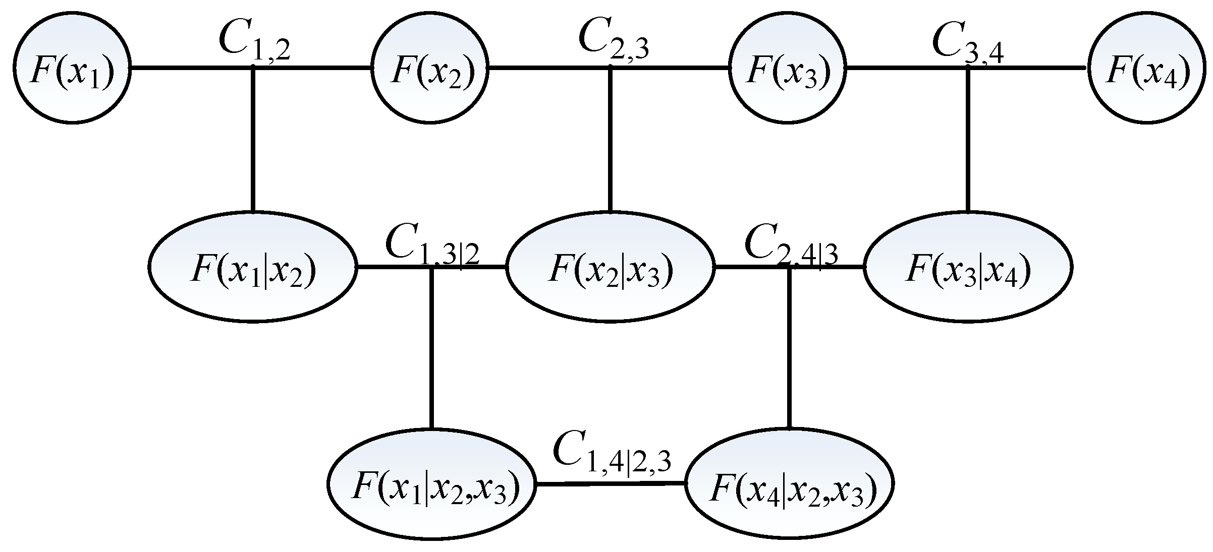
There is no dominant RV in the correlation modeling of the wind speed and load, so we adopt D-vine copulas to capture the dependence features. We then decompose Equation (8) as:

$$f(x_1,\dots ,x_n)={\displaystyle \prod _{i=1}^n{f}_i(x_i)}{\displaystyle \prod _{j=1}^{n-1}{\displaystyle \prod _{k=1}^{n-j}{c}_{k,k+j|k+1,\dots ,k+j-1}}}=D(x_1,\dots ,x_n){\displaystyle \prod _{i=1}^n{f}_i(x_i)},$$

(12)

where D(x₁, …, x_n) stands for the D-vine copula function.

Graphically, the D-vine structure adopted in Equation (12) can be illustrated by Figure 1, which is a 4-dimension case.

3.3.2. Parameter Estimation

We can choose a suitable copula type for each pair of F(x_k|x_k+1, …, x_k+j−1) and F(x_k+j|x_k+1, …, x_k+j−1) according to the property of their dependence, such as the tail behavior [39].

After the function form of each pair is determined, the parameter estimation process is carried out, in which we use the maximum log-likelihood estimation (MLE).

The MLE process proceeds row by row down the vine shown in Figure 1, because F(x_k|x_k+1, …, x_k+j−1) and F(x_k+j|x_k+1, …, x_k+j−1) are derived from the conditional copula CDF in the row above them by (11). The expression of MLE is:

$$\max \ln l(\Theta )={\displaystyle \prod _{y=1}^Y{\displaystyle \prod _{j=1}^{n-1}{\displaystyle \prod _{k=1}^{n-j}{c}_{k,k+j|k+1,\dots ,k+j-1}(F(x_k^y|x_{k+1}^y,\dots ,x_{k+j-1}^y),}}}F(x_{k+j}^y|x_{k+1}^y,\dots ,x_{k+j-1}^y);{\theta }_{k,k+j}),$$

(13)

where Y is the number of observations used for estimation. Θ is the set of all θ_k,k+j, which is the parameter of c_{k,k+j|k+1,…,k+j−1}.

After obtaining Θ by MLE, the expression of the joint PDF can be determined according to (12).

3.3.3. Generate Correlated Samples by D-Vine Copula

Consider x₁, …, x_n as the variables representing wind speed and load. In fact, when we use CE-IS to assess system reliability, only in the first iteration of the pre-simulation stage we may use D-vine copulas to draw samples. In the subsequent iterations, we draw samples from the suboptimal distribution derived by CE-IS. If there are enough historical observations, we can use the simple random sampling of the observations in the first iteration as well.

However, to ensure the integrity of the methodology, the procedures of sampling from D-vine copulas is briefed below, based on Quasi-Monte Carlo method [40].

Step 1: Generate n independent samples distributed uniformly on [0, 1], which are denoted by z₁, …, z_n.

Step 2: Set z₁ = F₁(x₁), z₂ = F(x₂|x₁), …, z_n = F(x_n|x₁, …, x_n−1). Convert z_i into x_i by the inverse function of F(x_i|x₁, …, x_i−1), which has been saved while the bivariate conditional copulas are constructed by (11). F₁(x₁) is the marginal CDF of x₁ modeled by SNMM.

When we evaluate the CC of wind energy, we use the data of wind power rather than wind speed. Hence, the wind speed samples are further transformed into the power of the WTG by:

$$P(x_i)=\{\begin{array}{ll}0& x_i\notin \left(v_{ci},v_{co}\right)\\ \frac{P_R(x_i{}^3-v_{ci}{}^3)}{(v_{co}{}^3-v_{ci}{}^3)}& x_i\in \left(v_{ci},v_r\right)\\ P_R& x_i\in \left(v_r,v_{co}\right)\end{array},$$

(14)

where v_ci, v_r and v_co are the cut-in, rated and cut-out wind speed of the WTG. x_i can stand for any element in {x₁, …, x_n} that represents wind speed. P_R is the rating of the WTG.

4. DRCE-IS Combined with D-Vine Copula and SNMM to Assess the Power System Reliability

The essence of CE-IS is to search for the optimal distribution for every RV, in order to reduce the variance of the reliability indices estimated by MCS. Based on the traditional CE-IS method, we propose the DRCE-IS method, which specifically aims at finding a better way to deal with the large numbers of 2- and 3-state units in the reliability assessment.

4.1. Overview of CE-IS

Denote all the RVs in reliability assessment by a vector x_ss, i.e.,

$$x_{ss}=[x^L,x^{CU},x^{WT},x^{LW}],$$

(15)

where x^L, x^CU and x^WT are the RV vectors representing the states of transmission lines, conventional units and WTGs. x^LW is the RV vector representing the values of the load and wind speed at different sites.

Then the reliability index γ can be determined by:

$$\gamma ={\displaystyle \int I(x_{ss})f(x_{ss};\theta )d{x}_{ss}},$$

(16)

where I(x_ss) is a function to indicate the system state, e.g., in the normal or failure states. f(x_ss;θ) is the original joint PDF of x_ss with θ as the parameter vector.

Equation (16) can be further transformed by the optimal joint PDF g(x_ss) used in importance sampling (IS), which is called IS PDF in this paper. The transformed (16) is shown as:

$$\gamma ={\displaystyle \int I(x_{ss})\frac{f(x_{ss};\theta )}{g(x_{ss})}}\cdot g(x_{ss})d{x}_{ss}=E_g\left[I(x_{ss})\frac{f(x_{ss};\theta )}{g(x_{ss})}\right],$$

(17)

where the rightmost term is an expectation in which g(x_ss) and I(x_ss)Q(x_ss) act as the PDF and a function of the RVs.

The theoretical expression of the optimal IS PDF is [28]:

$$g(x_{ss})=\frac{I(x_{ss})f(x_{ss};\theta )}{{\displaystyle \int I(x_{ss})f(x_{ss};\theta )d{x}_{ss}}}=\frac{I(x_{ss})f(x_{ss};\theta )}{\gamma },$$

(18)

where g(x_ss) is obviously entangled with γ, which means that the explicit expression of g(x_ss) is unavailable.

To solve the problem, the concept of cross entropy is introduced into the process of IS to form the traditional CE-IS method. The basic idea is to select a function form in advance, regardless of the actual form of the optimal PDF. Denote the selected function form as f(·;ω), in which ω is the parameter vector unknown. By minimizing the Kullback-Leibler (KL) divergence between f(·;ω) and g(·), we can derive a satisfactory suboptimal PDF as the IS PDF.

The KL divergence K(g, f) is expressed as:

$$K(g,f)={\displaystyle \int g(x_{ss})\ln g(x_{ss})d{x}_{ss}}-{\displaystyle \int g(x_{ss})\ln f(x_{ss};\omega )}d{x}_{ss}=C-{\displaystyle \int g(x_{ss})\ln f(x_{ss};\omega )}d{x}_{ss},$$

(19)

where the first integral term is independent of ω, so it can be regarded as a constant C when we search for the optimal ω.

Then, we plug (18) into (19) and get the objective function used for optimizing ω, shown as:

$$\omega =\underset{\omega }{\arg \min }K(g,f)=\underset{\omega }{\arg \min }\gamma K(g,f)=\underset{\omega }{\arg \max }{\displaystyle \int I(x_{ss})\ln f(x_{ss};\omega )f(x_{ss};\theta )}d{x}_{ss}.$$

(20)

The integral term in (20) can be further converted as:

$$\begin{array}{ll}\omega & =\underset{\omega }{\arg \max }{\displaystyle \int I(x_{ss})\frac{f(x_{ss};\theta )}{f(x_{ss};\omega )}f(x_{ss};\omega )\ln f(x_{ss};\omega )}d{x}_{ss}=\underset{\omega }{\arg \max }{E}_{\omega }\left[I(x_{ss})\frac{f(x_{ss};\theta )}{f(x_{ss};\omega )}\ln f(x_{ss};\omega )\right]\\ & =\underset{\omega }{\arg \max }{E}_{\omega }\left[I(x_{ss})Q(x_{ss})\ln f(x_{ss};\omega )\right]\approx \underset{\omega }{\arg \max }\frac{1}{n_s}{\displaystyle \sum _{s=1}^{n_s}I(x_{ss,s})Q(x_{ss,s})\ln f(x_{ss,s};\omega )},\end{array}$$

(21)

where E_ω(∙) stands for the expectation of a function with f(∙;ω) as the PDF. n_s is the sample size for estimating the expectation. Q(x_ss) is called the likelihood ratio function (LRF), which can be divided into several parts, shown as:

$$Q(x_{ss})=Q(x^L)Q(x^{CU})Q(x^{WT})Q(x^{LW}).$$

(22)

There is no constraint imposed on (21), so the best ω can be achieved when the derivative of the last term in (21) is equal to zero.

4.2. Pre-Simulation Stage of DRCE-IS

DRCE-IS consists of a pre-simulation stage and a main simulation stage. We detail the pre-simulation stage first. The purpose of the pre-simulation stage is to derive IS PDFs for continuous RVs and IS probability mass functions (PMF) for discrete RVs.

We use an iterative process to eliminate the randomness of the samples in (21). In each iteration, we draw n_s new samples from f(·;ω) to solve (21) again to renew f(·;ω) for the next iteration, until the terminating condition is satisfied.

IS PMFs, particularly, will hold the same function form as the original PMFs of the discrete RVs, while IS PDFs will be assigned a new function form, totally different from the original ones.

4.2.1. IS PMFs of Transmission Lines

The PMFs of the transmission lines are shown as:

$$p(x_l)={({\omega }_l)}^{1-x_l}{(1-{\omega }_l)}^{x_l}\hspace{1em}\hspace{1em}l=1,\dots ,n_L,$$

(23)

where ω_l is the optimal failure probabilities of transmission lines. x_l is the RV representing the states of the l-th transmission line, whose potential values are 0 and 1, indicating failure state and operation state, respectively. n_L is the number of transmission lines.

When we update ω_l, only the terms containing ω_l in (21) affect the IS PMF. Therefore, we retain them in the objective function, while other terms are replaced by a constant C. Then, the objective function is shown as:

$$\underset{{\omega }_l}{\max }{\displaystyle \sum _{s=1}^{n_s}I(x_{ss,s})Q(x_{ss,s})\ln p(x_{l,s})}+C=\underset{{\omega }_l}{\max }{\displaystyle \sum _{s=1}^{n_s}I(x_{ss,s})Q(x_{ss,s})\ln \left[{({\omega }_l)}^{1-x_{l,s}}{(1-{\omega }_l)}^{x_{l,s}}\right]}+C.$$

(24)

In the t-th iteration, draw n_s new samples and make the derivative of (24) equal to zero, i.e.,

$$\frac{1}{{\omega }_{l,t}}{\displaystyle \sum _{s=1}^{n_s}I(x_{ss,s})Q(x_{ss,s})(1-x_{l,s})}+\frac{1}{{\omega }_{l,t}-1}{\displaystyle \sum _{s=1}^{n_s}I(x_{ss,s})Q(x_{ss,s})x_{l,s}}=0.$$

(25)

The solution of (25) is the optimal failure probabilities of transmission lines, which is shown as:

$${\omega }_{l,t}=1-{\displaystyle \sum _{s=1}^{n_s}I(x_{ss,s})Q(x_{ss,s})x_{l,s}}/{\displaystyle \sum _{s=1}^{n_s}I(x_{ss,s})Q(x_{ss,s})}.$$

(26)

Equation (26) is valid for any l = 1, …, n_L. The set {x_l|l = 1, …, n_L} forms the vector x^L in (22). According to (21), LRF is defined as the ratio of the original PDF (or PMF) to the IS one. Hence, the LRF of transmission lines Q(x^L) is given as:

$$Q(x^L)={\displaystyle \prod _{l=1}^{n_L}{\left(1-{\theta }_l\right)}^{x_l}{\left({\theta }_l\right)}^{1-x_l}}/{\displaystyle \prod _{l=1}^{n_L}{\left(1-{\omega }_l\right)}^{x_l}{\left({\omega }_l\right)}^{1-x_l}},$$

(27)

where θ_l is the original failure probability of the transmission line l.

4.2.2. IS PMFs of Homogeneous 2- and 3-State Units

The wind farms in this paper are all centralized and integrated with the transmission network, which means that the WTGs on the same wind farm are definitely connected to the same bus in the power system. Hence, the WTGs of the same type on the same wind farm make equal contributions to the power system. These WTGs should have the same IS PMF. Similarly, the 2-state conventional units, which are of the same type and connected to the same bus, should have the same IS PMF. These units/WTGs are called “homogeneous units” in this paper.

If we search for the IS PMFs of the homogeneous units individually, the IS PMFs may significantly differ from each other due to the randomness of the samples, which are also far away from the theoretical optimal PMF. Besides, the state of each unit is regarded as a RV, which results in a high-dimension problem and a bulky solution space, increasing the difficulty and time in searching for optimal PMFs.

To solve the problem, we aggregate the homogeneous units into a single group and represent the group by one RV. For the group of 2-state conventional units, the RV follows binomial distribution, while for the group of 3-state WTGs, the RV obeys trinomial distribution.

By this means, the dimension of the solution space is reduced, which improves the quality of the IS PMFs.

Denote the number of 2-state conventional units in the c-th group as n_c. The failure probability is marked as ω_f,c. Denote x_f,c as the number of units in the failure state in the c-th group. The PMF of the c-th group p(x_c) is shown as:

$$p(x_c)=\frac{n_c!{({\omega }_{f,c})}^{x_{f,c}}{(1-{\omega }_{f,c})}^{x_{f,c}}}{x_{f,c}!(n_c-x_{f,c})!},$$

(28)

where x_c = [x_f,c, n_c − x_f,c].

When we update ω_f,c, we only retain the terms containing ω_f,c in the objective function, i.e.,

$$\underset{{\omega }_f{}_{,c}}{\max }{\displaystyle \sum _{s=1}^{n_s}I(x_{ss,s})Q(x_{ss,s})\ln p(x_{c,s})}+C.$$

(29)

Similarly with the processing of transmission lines, we can obtain the solution of (29), which is the updating formulae for ω_f,c, shown as:

$${\omega }_f{}_{,c,t}={\displaystyle \sum _{s=1}^{n_s}I(x_{ss.s})Q(x_{ss,s})x_{f,c,s}}/n_c{\displaystyle \sum _{s=1}^{n_s}I(x_{ss,s})Q(x_{ss,s})}.$$

(30)

Equation (30) is valid for any c = 1, …, n_cg. n_cg is the number of conventional unit groups.

The set {x_c|c = 1, …, n_cg} forms the vector x^CU in (22). Then the LRF of conventional units Q(x^CU) can be expressed as:

$$Q(x^{CU})={\displaystyle \prod _{c=1}^{n_{cg}}{\left({\theta }_{f,c}\right)}^{x_{f,c}}{\left(1-{\theta }_{f,c}\right)}^{n_c-x_{f,c}}}/{\displaystyle \prod _{c=1}^{n_{cg}}{\left({\omega }_f{}_{,c}\right)}^{x_{f,c}}{\left(1-{\omega }_f{}_{,c}\right)}^{n_c-x_{f,c}}},$$

(31)

where θ_f,c is the original failure probability of the c-th group of conventional units.

Denote the number of 3-state WTGs in the w-th group as n_w. The failure and derated probabilities are marked as ω_f,w and ω_d,w, respectively. The PMF of the w-th group p(x_w) is shown as:

$$p(x_w)=\frac{n_w!{({\omega }_{f,w})}^{x_{f,w}}{({\omega }_{d,w})}^{x_{d,w}}{({\omega }_{o,w})}^{x_{o,w}}}{x_{f,w}!x_{d,w}!x_{o,w}!},$$

(32)

where x_w = [x_f,w, x_d,w, x_o,w]. x_f,w, x_d,w and x_o,w are the number of WTGs in the failure, derated and operation states in the w-th group, respectively, which meet:

$${\eta }_{o,w}=1-{\omega }_{f,w}-{\omega }_{d,w},x_{o,w}=n_w-x_{f,w}-x_{d,w}.$$

(33)

Similarly with (24), when we update ω_f,w and ω_d,w, the objective function is shown as:

$$\underset{{\omega }_{f,w},{\omega }_{d,w}}{\max }{\displaystyle \sum _{s=1}^{n_s}I(x_{ss,s})Q(x_{ss,s})\ln p(x_{w,s})}+C.$$

(34)

Similarly with (26), the solutions of (34) are the updating formulae for ω_f,w and ω_d,w, which are shown as:

$${\omega }_{f,w,t}=\frac{(1-{\omega }_{d,w,t-1}){\displaystyle \sum _{s=1}^{n_s}I(x_{ss,s})Q(x_{ss,s})x_{f,w,s}}}{{\displaystyle \sum _{s=1}^{n_s}I(x_{ss,s})Q(x_{ss,s})(n_w-x_{d,w,s})}},$$

(35)

$${\omega }_{d,w,t}=\frac{(1-{\omega }_{f,w,t-1}){\displaystyle \sum _{s=1}^{n_s}I(x_{ss,s})Q(x_{ss,s})x_{d,w,s}}}{{\displaystyle \sum _{s=1}^{n_s}I(x_{ss,s})Q(x_{ss,s})(n_w-x_{f,w,s})}}.$$

(36)

Equations (35) and (36) is valid for any w = 1, …, n_wg. n_wg is the number of WTG groups.

The set {x_w|w = 1, …, n_wg} forms x^WT in (22). Then the LRF of WTGs Q(x^WT) is expressed as:

$$Q(x^{WT})=\frac{{\displaystyle \prod _{w=1}^{n_{wg}}{\left({\theta }_{f,w}\right)}^{x_{f,w}}{\left({\theta }_{d,w}\right)}^{x_{d,w}}{\left({\theta }_{o,w}\right)}^{x_{o,w}}}}{{\displaystyle \prod _{w=1}^{n_{wg}}{\left({\omega }_{f,w}\right)}^{x_{f,w}}{\left({\omega }_{d,w}\right)}^{x_{d,w}}{\left({\omega }_{o,w}\right)}^{x_{o,w}}}},$$

(37)

where θ_f,w, θ_d,w and θ_o,w are the original state probabilities of the w-th WTG group.

We only deal with 2- and 3-state units in this paper. However, the proposed method is not limited to 2- and 3-state units. The method can be expanded to the case of multi-state units by replacing p(x_c) and p(x_w) with the PMF of the multinomial distribution, so it is widely adaptive.

4.2.3. IS PDF of the Wind Speed and Load Based on D-Vine Copulas and SNMM

Load and wind speed are represented by continuous RVs, so we need to acquire the IS joint PDF, rather than the PMF. According to the basic idea of CE-IS, there is no restriction to f(·;ω) in (19). Actually whatever the form of f(·;ω) is, we can obtain a practical IS PDF by optimizing ω.

For simplicity, we select the multivariate Gaussian PDF as the IS joint PDF, in which all variables are supposed to be independent. The expectation μ^LW and standard deviation σ^LW are the parameters to be optimized, just like ω in (19). Therefore, when we update μ^LW and σ^LW, the objective function can be represented by:

$$\underset{{\mu }^{LW},{\sigma }^{LW}}{\max }{\displaystyle \sum _{s=1}^{n_s}I(x_{ss,s})Q(x_{ss,s})\ln \phi (x_s^{LW};{\mu }^{LW},diag({\sigma }^{LW}))}+C,$$

(38)

where diag(∙) is a transformation by which a vector is converted into a diagonal matrix.

Similarly, with the processing of the PMFs, (38) is solved, whose solutions are the updating formulae for μ^LW and σ^LW, shown as:

$${\mu }_t^{LW}={\displaystyle \sum _{s=1}^{n_s}I(x_{ss,s})Q(x_{ss,s})x_s^{LW}}/{\displaystyle \sum _{s=1}^{n_s}I(x_{ss,s})Q(x_{ss,s})},$$

(39)

$${\left({\sigma }_t^{LW}\right)}^{\circ 2}=\frac{{\displaystyle \sum _{s=1}^{n_s}I(x_{ss,s})Q(x_{ss,s}){\left(x_s^{LW}-{\mu }_t^{LW}\right)}^{\circ 2}}}{{\displaystyle \sum _{s=1}^{n_s}I(x_{ss,s})Q(x_{ss,s})}},$$

(40)

where (·)°² stands for the Hadamard square.

The LRF of wind speed and load is defined based on the D-vine copulas and SNMM, because we need to combine them to obtain the original joint PDF. The LRF is expressed as:

$$Q(x^{LW})=D(x^{LW}){\displaystyle \prod _{lw=1}^{n_{lw}}{f}_{lw}(x_{lw})}/\phi (x^{LW};{\mu }^{LW},diag({\sigma }^{LW})),$$

(41)

where n_lw is the number of RVs of wind speed and load. f_lw(·) is the marginal PDF modeled by SNMM.

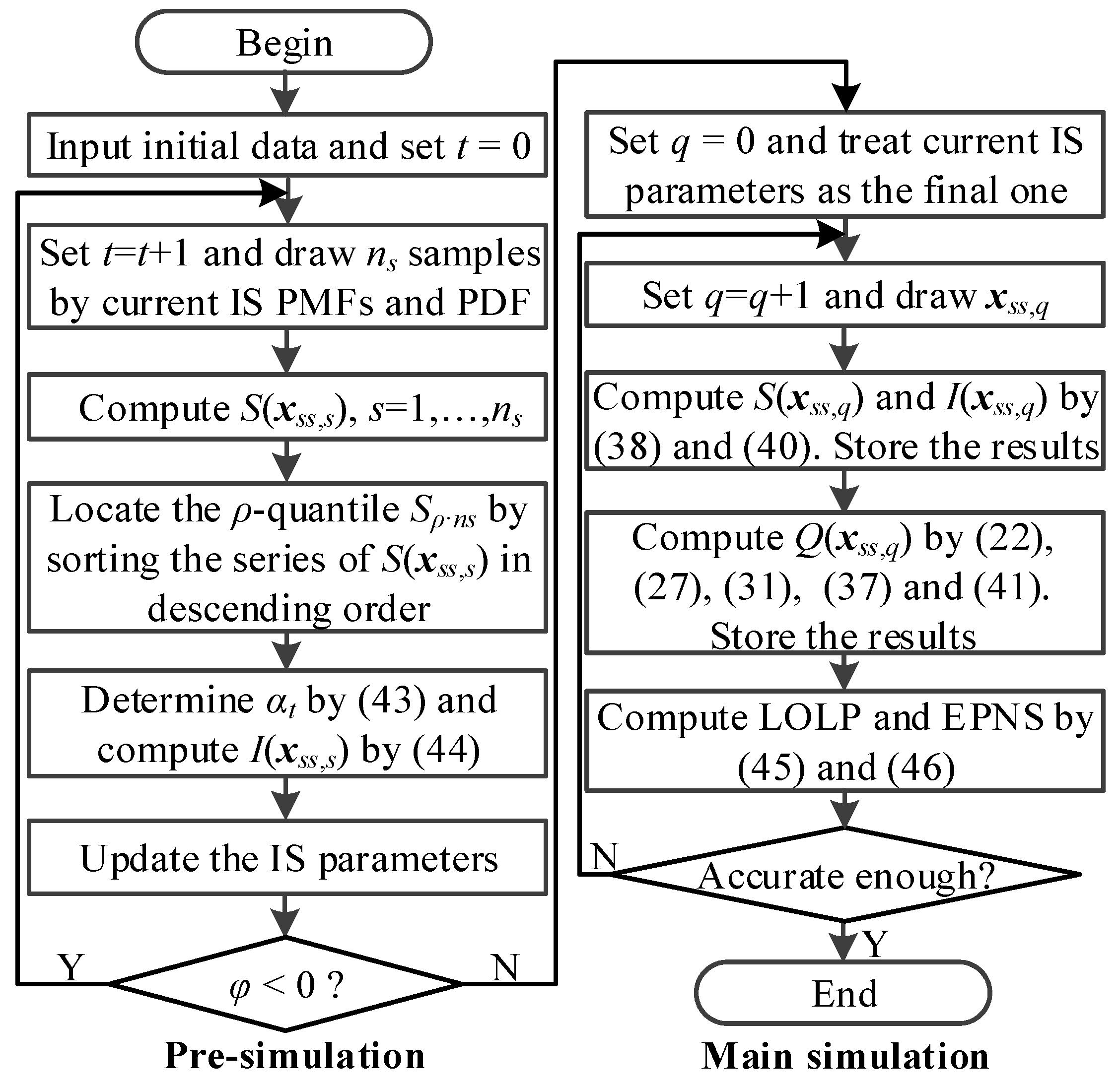
4.2.4. Procedures of Pre-Simulation Stage

The procedures of the pre-simulation stage are detailed as below.

Step 1: Input the original PMFs and joint PDF of RVs in the reliability assessment. Set t = 0. Specify the sample size n_s in each iteration.

Step 2: In the t-th iteration, draw n_s new samples by using {ω_l,t|l = 1, …, n_L}, {ω_f,c,t|c = 1, …, n_c}, {ω_f,w,t, ω_d,w,t|w = 1, …, n_w}, μ_t^LW and σ_t^LW. Denote the samples by {x_ss,s|s = 1, …, n_s}.

Step 3: Quantify the performance of each sample in the term of reliability. The frequently used quantifying method is the minimum load shedding (MLS) model, whose objective function is the quantifying function S(x_ss,s).

The MLS model is expressed as:

$$\begin{array}{l}\underset{{\mathit{P}}_{\mathit{sh}},{\mathit{P}}_{\mathit{g}},\mathit{\delta }}{\min }S({\mathit{x}}_{ss,s})=1^T{\mathit{P}}_{\mathit{sh}}\\ s.t.\{\begin{array}{l}{1}^T{\mathit{P}}_{\mathit{g}}-1^T{\mathit{P}}_{\mathit{d}}+1^T{\mathit{P}}_{\mathit{sh}}=0\\ {\mathit{P}}_{\mathit{g}\min }\le {\mathit{P}}_{\mathit{g}}\le {\mathit{P}}_{\mathit{g}\max }\\ 0\le {\mathit{P}}_{\mathit{sh}}\le {\mathit{P}}_{\mathit{d}}\\ -{\mathit{P}}_{\mathit{line}\max }\le \mathit{bA}\mathit{\delta }\le {\mathit{P}}_{\mathit{line}\max }\\ {\mathit{A}}^T\mathit{bA}\mathit{\delta }={\mathit{P}}_{\mathit{g}}+{\mathit{P}}_{\mathit{sh}}-{\mathit{P}}_{\mathit{d}}\end{array},\end{array}$$

(42)

where P_g, P_sh and δ are the control variable of the model. P_g is the vector of generation power at all buses including wind power, whose upper and lower limits are P_gmax and P_gmin. P_sh is the vector of load shedding amount at all buses. δ is the vector of the voltage phase angle of all buses. P_d is the vector of the load demand at all buses. b is a diagonal matrix, whose diagonal elements are the reciprocal of the reactance of all transmission lines. A is the branch-node association matrix. P_linemax is the vector of maximum transmission capacity of all lines.

Step 4: Sort the performance of {x_ss,s|s = 1, …, n_s} and obtain a series {S₁, S₂, …, S_ns}, where S₁ ≥ S₂ ≥…≥ S_ns. Locate the ρ-quantile of the series and denote it as S_ρ·ns.

Step 5: In the t-th iteration, set a threshold α_t for {S₁, S₂, …, S_ns} by:

$${\alpha }_t=\{\begin{array}{l}0S_{\rho \cdot ns}>0\\ S_{\rho \cdot ns}{S}_{\rho \cdot ns}\le 0\end{array}.$$

(43)

According to the value of α_t, we can define the system state I(x_ss,s) as:

$$I(x_{ss,s})=\{\begin{array}{l}1\mathrm{if}S(x_{ss,s})>{\alpha }_t\\ 0\mathrm{if}S(x_{ss,s})\le {\alpha }_t\end{array}.$$

(44)

Step 6: By (26), (30), (35), (36), (39) and (40), we can update the parameters of the IS PMFs and IS PDF with the samples generated in Step 2 and the system states obtained in Step 5.

Step 7: If α_t = 0, end the pre-simulation stage and switch to the main simulation stage. Otherwise, set t = t + 1 and return to Step 2.

The pre-simulation procedures are shown in Figure 2.

4.3. Main Simulation Stage of DRCE-IS

The main simulation stage is implemented by adding a scaling operation to the MCS, which is to use the LRF Q(x_ss,s) to multiply the I(x_ss,s). The procedures are detailed as follows.

Step 8: Set the counter q = 0. The PMFs and PDF in the last iteration of the pre-simulation stage is accepted here.

Step 9: q = q + 1. Generate a new sample x_ss,q with the IS PMFs and PDF.

Step 10: Compute S(x_ss,q) by (42). Evaluate the system state by (44) with α_t = 0. Store the results.

Step 11: Compute Q(x_ss,q) by (22), (27), (31), (37) and (41). Store the results.

Step 12: Derive the reliability indices, the loss of load probability (LOLP) and expected power not supplied (EPNS) according to the stored data by:

$$\mathrm{LOLP}=\frac{1}{q}{\displaystyle \sum _{s=1}^{q}I(x_{ss,s})Q(x_{ss,s})},$$

(45)

$$\mathrm{EPNS}=\frac{1}{q}{\displaystyle \sum _{s=1}^{q}S(x_{ss,s})Q(x_{ss,s})}.$$

(46)

Step 13: Calculate the relative error of LOLP and EPNS. Compare them with the relative error limit. If LOLP and EPNS are accurate enough, end the algorithm and output them. Otherwise, return to Step 9.

The main simulation process is also shown in Figure 2.

5. Capacity Credit Assessment of Wind Energy by the Secant Method

The CC of wind energy is frequently defined as the equivalent load carrying capacity (ELCC) [41]. The ELCC is the load increment that is needed to maintain the reliability level unchanged after wind energy integration. The load increment is defined as the CC of the wind energy. The idea of ELCC is expressed as:

$$I(G,L)=I(G+\Delta G,L+\Delta L),$$

(47)

where I(·) is LOLE, EENS or other reliability indices. G and L are the total generation capacity and load demand of the whole system, respectively.

ΔG stands for the wind energy to be evaluated. ΔL is the load increment that the power system can support due to the integration of the wind energy.

Therefore, we need to find the maximum value of ΔL, which is usually implemented by the secant method [11]. The schematic diagram of the secant method is shown in Figure 3.

In the secant method, we need to compute the reliability index of the original system, which excludes the wind energy to be evaluated. The value of this index is denoted as R₀. Then we add the wind energy to form the new system and start an iterative process to compute the CC value.

From the schematic diagram, one can perceive that the points X_r and X_r+1 in the secant method are approaching the terminal point, whose ordinate is R₀. Actually, once the position of the terminal point is located, its abscissa minus L is the CC of the wind energy.

The procedures of the secant method are detailed below.

Step 1: Set r = 0. Determine two points X₀ and B by computing the reliability index with the load demands of the new system being L and L + ΔG, respectively.

Step 2: Connect X_r and B with a straight line, in which we search for a point whose ordinate is R₀. The abscissa of this point is defined as L_r+1.

Step 3: Find the new point X_r+1 by computing the reliability index with the load of the new system being L_r+1.

Step 4: If the ordinate of X_r+1 is not close enough to R₀, set r = r + 1 and return to Step 2. Otherwise, end the iteration. Output the value of the last L_r minus L, which is just ΔL in (47). ΔL is the CC of the wind energy.

The flowchart of the whole procedures is also presented in Figure 3.

6. Numerical Tests and Discussion

6.1. Simulation Setting

All tests are coded with MATLAB 2016a and run on an Intel Core i7-5500U personal computer with 16 G memory. We use LOLP and EPNS as the reliability indices.

In the test cases, the MCS method and traditional CE-IS method are compared with the DRCE-IS method in a modified IEEE-RTS 79 system. The data of the original IEEE-RTS 79 system can be acquired in [42]. The loads at all buses are expected to be perfectly positively related.

Four wind farms are integrated into the modified system. We arbitrarily connect them to Bus 1, 2, 13 and 21, respectively. Each of them includes 50 3MW-WTGs of the same type, whose parameters are shown in

Table 1. Reliability parameters of the 3MW-WTGs.

Parameter	Value	Parameter	Value
λf/(a−1)	7.96	derated ratio	60%
μf/(a−1)	58.4	vci/(m/s)	3
λd/(a−1)	5.84	vr/(m/s)	10
μd/(a−1)	43.8	vco/(m/s)	25

[43].

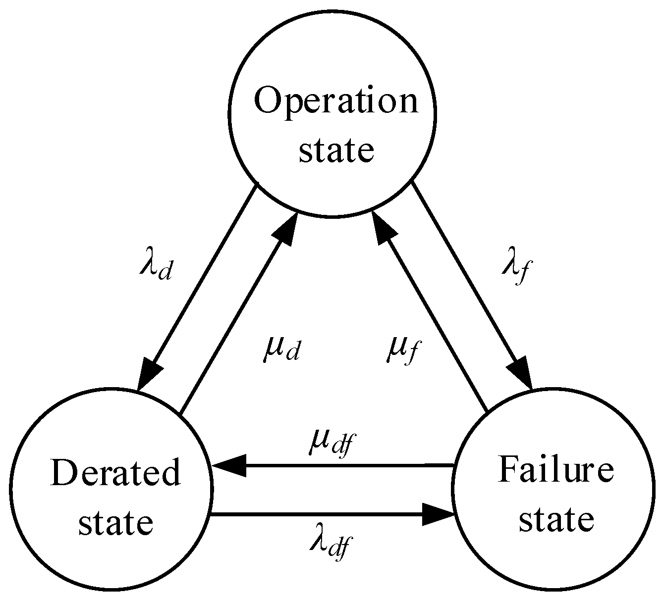
WTGs may work under operation, derated or failure states. λ_f, μ_f, λ_d, μ_d, λ_df and μ_df are the transition rates between any two of the three states, as shown in Figure 4. Theoretically, the WTG can transition from any of the three states to another, as shown by Figure 4. However, according to the “partial failure mode” developed in Page 26–27 of [44], WTGs are always restored to the operation state rather than the derated state in the actual repair process, so it is difficult to obtain λ_df and μ_df by statistics. Hence, the transfer between the derated and failure states is always omitted. We also employ the assumption and set λ_df and μ_df as zero here.

Under the assumption, the probabilities of failure and derated states are derived by:

$${\theta }_d=\frac{{\mu }_f{\lambda }_d}{{\lambda }_d{\mu }_f+{\mu }_d{\mu }_f+{\lambda }_f{\mu }_d},{\theta }_f=\frac{{\mu }_d{\lambda }_f}{{\lambda }_d{\mu }_f+{\mu }_d{\mu }_f+{\lambda }_f{\mu }_d},$$

(48)

where θ_f is the failure probability and θ_d is the derated probability, which are consistent with the notation in (37).

According to the data in Table 1, we can calculate θ_d and θ_f, which are 0.1050 and 0.1074, respectively.

According to the practical experience in the wind farms in Northwest China [43], the output of WTGs under derated state is set as 60–70% of its real-time maximum available output. Hence, we set the derated ratio as 60%, shown in Table 1.

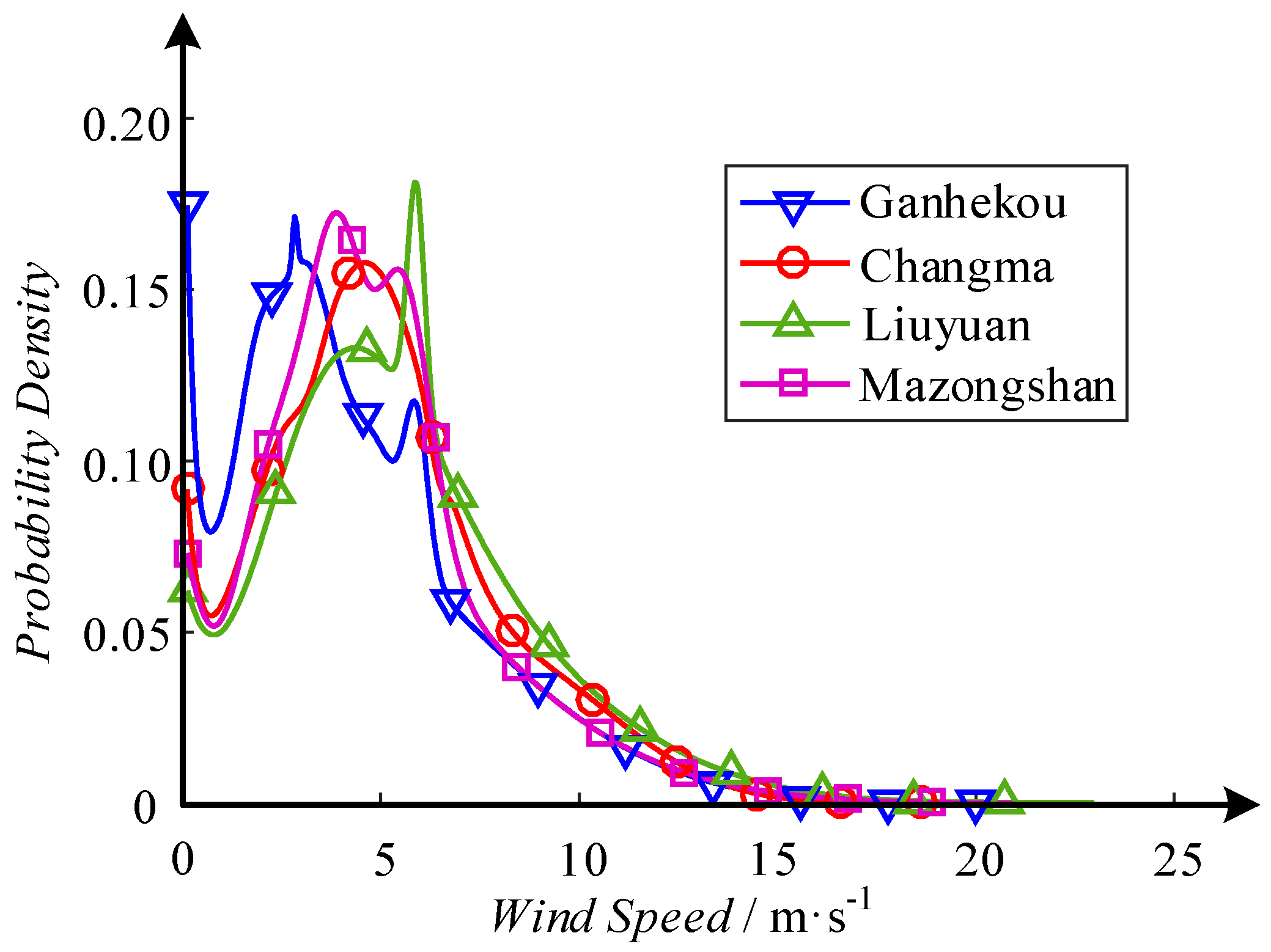
Wind speed data at Bus 1, 2, 13 and 21 are extracted from the historical data of four areas in Northwest China from 1 January to 31 December in 2013. The areas are Ganhekou, Changma, Liuyuan and Mazongshan. The wind speed PDFs are shown as curves in Figure 5. The data can be referred to by DOI: 10.13140/RG.2.2.29281.97125.

6.2. Verification of the Proposed Methods

6.2.1. Validation of SNMM

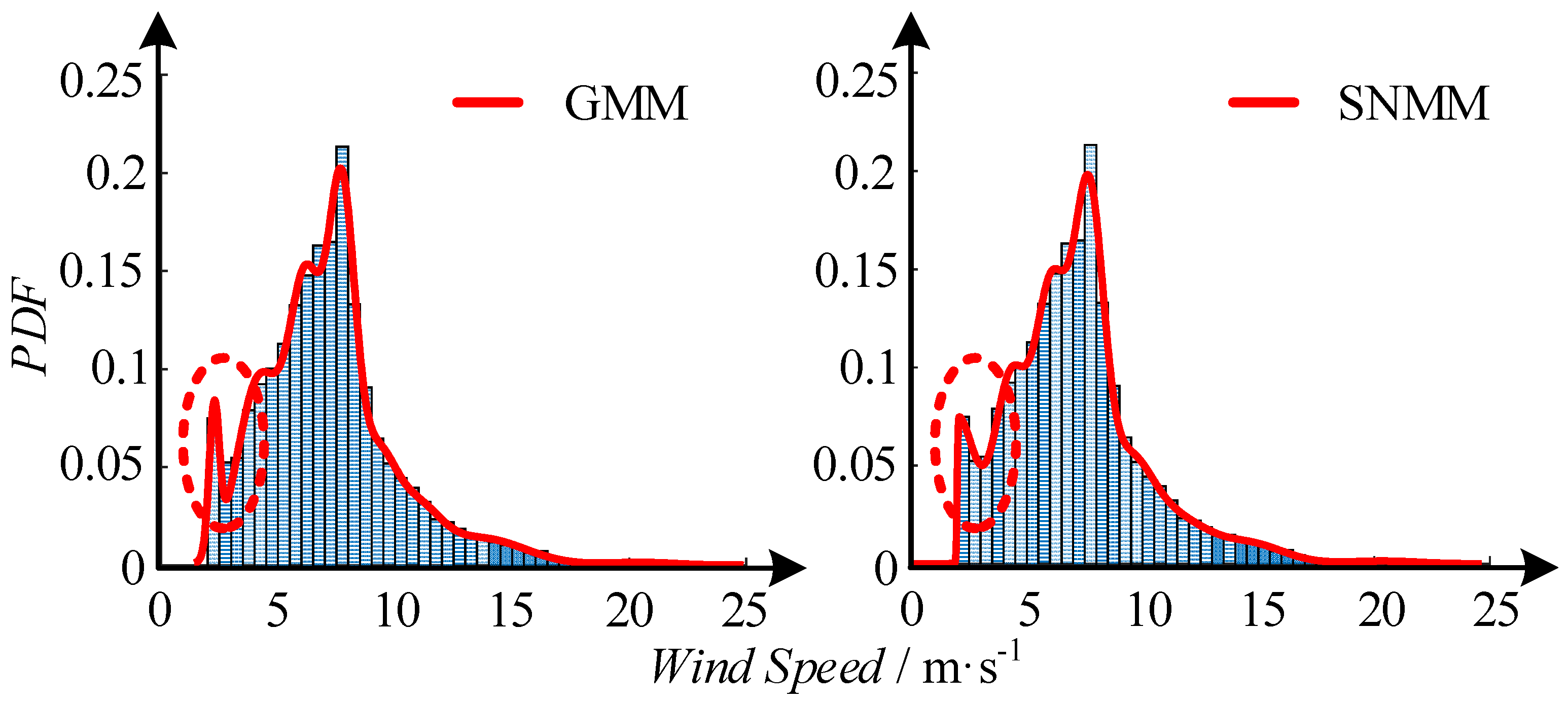
Before using SNMM and D-vine copulas to provide scenarios for reliability assessment, we need to validate them. Firstly, we use the wind speed data at Mazongshan as an example to illustrate the performance of SNMM.

The fitted PDF by using GMM and SNMM with eight components is depicted in Figure 6, respectively. A distinct difference between the two PDFs is marked by a red dashed circle, which shows that SNMM performs better than GMM when they have the same number of components.

To present the superiority quantitatively, we compute the Chi-square values of the models fitted by SNMM, GMM [45], Weibull model and kernel density estimation (KDE) [46], as shown in

Table 2. Chi-square values of three models.

	SNMM	GMM	Weibull	KDE
BUS 1	33.45	93.65	9907.10	213.53
BUS 2	20.15	39.17	421.69	94.90
BUS 13	27.73	62.53	1452.37	84.06
BUS 21	51.42	67.22	6611.95	123.53

.

Apparently, SNMM holds the minimum Chi-square values among the three for all wind speed. Hence, SNMM is validated and can be further used to model the marginal PDFs of wind speed and load in reliability assessment.

6.2.2. Validation of D-Vine Copulas

Since the load at all buses is perfectly positively correlated, there are five correlated RVs in the test system, i.e., the wind speed at four sites and the total load of the system.

We apply D-vine copulas to construct the correlation model based on historical data. Each bivariate copula can be chosen from Normal, Student t, Clayton, Gumbel, Frank and Joe copulas, whose parameters are shown in

Table 3. Parameters of the constructed D-vine copulas.

Copula	Types	Para1	Para2	AIC	BIC
c12	Joe	1.27	0	−621.86	−614.79
c23	Joe	1.47	0	−1462.92	−1455.85
c34	Joe	1.17	0	−291.79	−284.71
c45	Normal	−0.03	0	−5.15	1.93
c13|2	Joe	1.85	0	−3132.12	−3125.05
c24|3	Gumbel	1.34	0	−1666.12	−1659.05
c35|4	Joe	1.02	0	−8.93	−1.85
c14|23	Student t	−0.15	13.07	−263.15	−249.00
c25|34	Normal	−0.05	0	−20.21	−13.14
c15|234	Student t	0.00	26.16	−9.38	−2.30

.

To evaluate the goodness-of-fit of D-vine copulas, we use the statistic recommended by [47], which is based on Cramér-Von Mises (CvM) criterion and empirical copula process (ECP). We entitle it ECP-CvM, which indicates the difference between the fitted model and the empirical model.

The ECP-CvMs of D-vine copulas, C-vine copula [27], Normal copula and t copula are calculated and shown in

Table 4. Comparison of ECP-CvMs of three copula models.

Copula model	D-vine	C-vine	Normal	t
ECP-CvM	6.9377	9.1743	203.8986	208.2088

.

According to the results in Table 4, D-vine copulas exhibit superiority over Normal and t copulas due to a much smaller ECP-CvM value. It performs much better than any individual multivariate copula model, so we can adopt it for reliability assessment of power systems.

6.2.3. Validation of DRCE-IS

In this section, we validate the DRCE-IS method by comparing the values of LOLP and EPNS obtained by MCS, CE-IS [28] and DRCE-IS. Then the CC for wind farms will be evaluated by the DRCE-IS and the secant method.

Relevant parameters of DRCE-IS are set as follows:

(1)

n_s in Step 1 of the pre-simulation stage is 50,000.

(2)

ρ in the Step 4 of the pre-simulation stage is 0.05.

(3)

The relative error limit in the main simulation stage is set as 0.05 for both LOLP and EPNS.

Based on the parameters above, we can assess the reliability of power systems with the four integrated wind farms, whose values are displayed in

Table 5. Reliability indices of the modified IEEE-RTS 79 system with four dependent wind farms.

	LOLP/10−4	Sample Size	EPNS/MW	Sample Size
MCS	1.9455	3,066,720	0.0214	7,574,343
CE-IS	1.9774	14,540	0.0209	8916
DRCE-IS	1.9549	9374	0.0213	4709

.

Since the LOLP and EPNS values obtained by the three methods are remarkably close to each other under the same relative error limit 0.05, we conclude that DRCE-IS is correct. Besides, the sample size of DRCE-IS is smaller than that of CE-IS, because of the proposed DR technique. Hence, the DRCE-IS is validated.

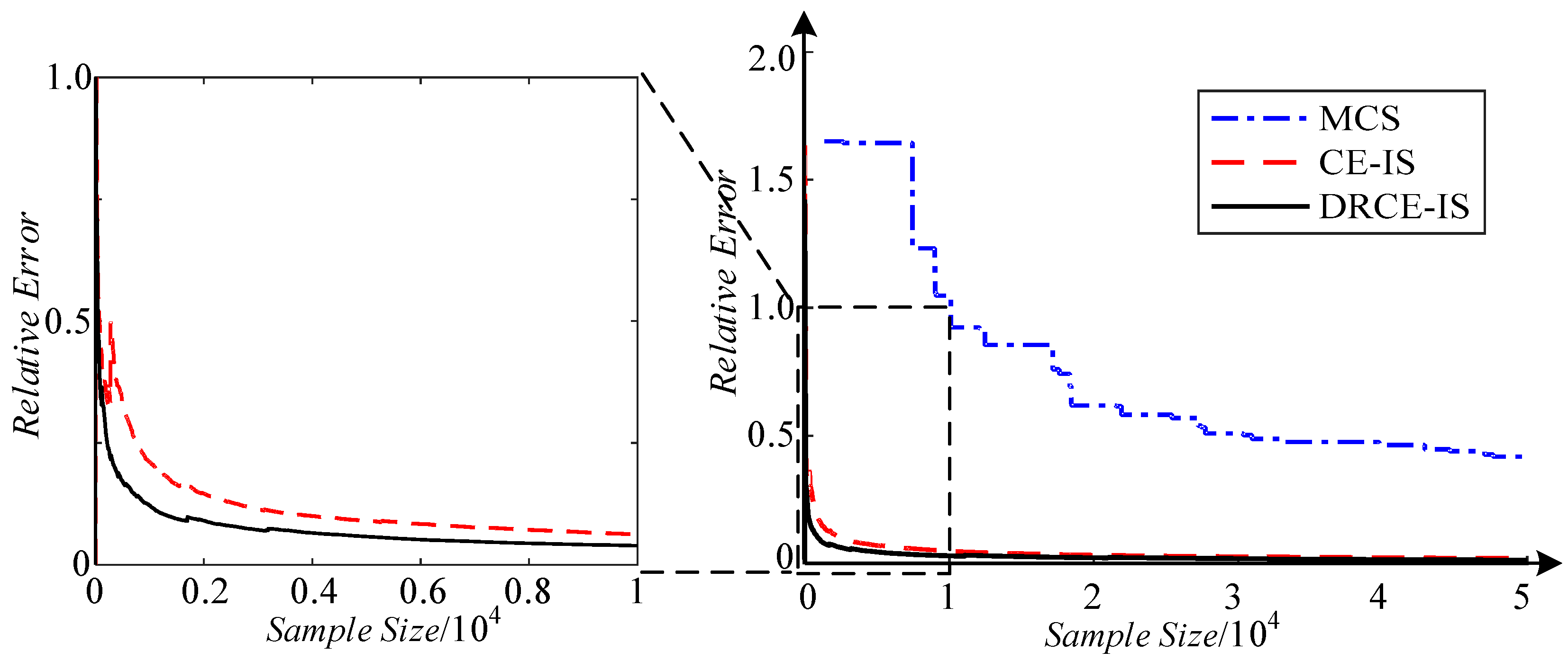
The convergence process of the three methods is depicted in Figure 7. The ordinate is the relative error of the LOLP computed by samples. With the increase of sample size, the errors of the three all decrease. One can perceive that the relative error of DRCE-IS is the first to decrease to 0.05, which is also consistent with the results in Table 5.

6.3. Evaluate the Capacity Credit of Wind Energy by DRCE-IS and the Secant Method

Finally, we can calculate the CC of the four wind farms with the secant method and all the methods validated above. The parameters of DRCE-IS is exactly the same as those in Section 6.2.3.

According to Figure 3, we need to compute the reliability indices in three distinct situations to start the iteration of the secant method, which correspond to R_d, R_u and R₀ in Figure 3.

We employ LOLP to compute R_d, R_u and R₀, whose values are listed with the CC of each wind farm in

Table 6. Three LOLP values and CC of four wind farms.

	R0/10−4	Rd/10−4	Ru/10−4	CC/MW	CCF/%
W1	2.5544	1.9227	5.6365	37.361	24.91
W2	2.5304	1.9246	5.5950	35.477	23.65
W3	1.9614	1.6219	4.8975	24.116	16.07
W4	2.4687	1.6075	4.8615	39.925	26.62

.

Besides, we also compute the ratio of CC of each wind farm to its installed capacity, which is called capacity credit factor (CCF). Since the installed capacity of each wind farm is 3 × 50 = 150 MW, we can easily obtain the CCF values, shown in Table 6 as well.

The results in Table 6 unveil the fact that the CCF of wind energy is rather small (below 30%), which reflects a low efficiency in utilizing wind energy. This is definitely due to the characteristics of uncertainty and fluctuation of wind. Therefore, how to overcome the disadvantages to improve the CCF of wind energy by available measures, such as by energy storage systems and demand response dispatch, will be researched in our future work.

7. Conclusions

This paper focuses on the capacity credit evaluation of wind energy, whose key points are modeling the uncertainty of the correlated wind speed and load and assessing the power system reliability. The main achievements and conclusions are listed below:

(1)

A novel method of fitting the joint PDF is proposed for wind speed and load. Particularly, SNMM is used to fit the marginal PDFs, while the correlation model is established by D-vine copulas.

(2)

The goodness-of-fit of SNMM, GMM, Weibull model and KDE is quantified by the Chi-square values, among which that of SNMM is the smallest. Similarly, the goodness-of-fit of D-vine, C-vine, Normal and t copulas is quantified by the ECP-CvM values, among which that of D-vine is the smallest. Therefore, SNMM and D-vine copulas are validated.

(3)

DRCE-IS is developed to enhance the efficiency of power system reliability assessment by proposing the idea of “homogeneous units” The convergence of reliability indices using DRCE-IS is remarkably faster than that using traditional CE-IS and MCS without compromising accuracy.

(4)

Based on the wind speed data obtained in Northwest China, we integrate four wind farms into IEEE-RTS 79 system, whose CC values are evaluated by the combination of SNMM, D-vine copulas, DRCE-IS and the secant method. The CCF values of four wind farms, which means the ratio of their CC to the installed capacity, are all below 30%, which indicates a failure to make full use of wind energy. Hence, how to improve the CC of wind energy is worth further research.

References

- Cao, M.; Qingshan, X.; Nazaripouya, H.; Chu, C.; Pota, H.; Gadh, R. An Engineering Energy Storage Sizing Method Considering the Energy Conversion Loss on Facilitating Wind Power Integration. IET Gener. Transm. Distrib. 2018. to be published. [Google Scholar] [CrossRef]
- Wang, Y.; Shi, W.; Wang, B.; Chu, C.; Gadh, R. Optimal operation of stationary and mobile batteries in distribution grids. Appl. Energy 2017, 190, 1289–1301. [Google Scholar] [CrossRef] [Green Version]
- Zang, H.; Cheng, L.; Ding, T.; Cheung, K.W.; Liang, Z.; Wei, Z.; Sun, G. Hybrid method for short-term photovoltaic power forecasting based on deep convolutional neural network. IET Gener. Transm. Distrib. 2018, 12, 4557–4567. [Google Scholar] [CrossRef]
- Wang, D.; Lu, K. Design optimization of hydraulic energy storage and conversion system for wave energy converters. Protect. Control Mod. Power Syst. 2018, 3, 70–78. [Google Scholar] [CrossRef]
- Minh, Q.D.; Leva, S.; Mussetta, M.; Le, K.H. A Comparative Study on Controllers for Improving Transient Stability of DFIG Wind Turbines During Large Disturbances. Energies 2018, 11, 480. [Google Scholar] [Green Version]
- Duong, M.Q.; Grimaccia, F.; Leva, S.; Mussetta, M.; Le, K.H. Hybrid controller for transient stability in wind generators. In Proceedings of the 2015 Clemson University Power Systems Conference (PSC), Clemson, SC, USA, 10–13 March 2015; Institute of Electrical and Electronics Engineers Inc.: Piscataway, NJ, USA, 2015. [Google Scholar]
- Li, J.; Wang, S.; Ye, L.; Fang, J. A coordinated dispatch method with pumped-storage and battery-storage for compensating the variation of wind power. Protect. Control Mod. Power Syst. 2018, 3, 21–34. [Google Scholar] [CrossRef]
- Voorspools, K.R.; D’Haeseleer, W.D. An analytical formula for the capacity credit of wind power. Renew. Energy 2006, 31, 45–54. [Google Scholar] [CrossRef]
- Keane, A.; Milligan, M.; Dent, C.J.; Hasche, B.; D’Annunzio, C.; Dragoon, K.; Holttinen, H.; Samaan, N.; Soeder, L.; O’Malley, M. Capacity Value of Wind Power. IEEE Trans. Power Syst. 2011, 26, 564–572. [Google Scholar] [CrossRef] [Green Version]
- Dent, C.J.; Keane, A.; Bialek, J.W. Simplified methods for renewable generation capacity credit calculation: A critical review. In Proceedings of the IEEE PES General Meeting, Providence, RI, USA, 25–29 July 2010; pp. 1–8. [Google Scholar]
- Ding, M.; Xu, Z. Empirical Model for Capacity Credit Evaluation of Utility-Scale PV Plant. IEEE Trans. Sustain. Energy 2017, 8, 94–103. [Google Scholar] [CrossRef]
- Parastegari, M.; Hooshmand, R.; Khodabakhshian, A.; Zare, A. Joint operation of wind farm, photovoltaic, pump-storage and energy storage devices in energy and reserve markets. Int. J. Electr. Power Energy Syst. 2015, 64, 275–284. [Google Scholar] [CrossRef]
- Albadi, M.H.; El-Saadany, E.F. Comparative Study on Impacts of Power Curve Model on Capacity Factor Estimation of Pitch-Regulated Turbines. J. Eng. Res. 2012, 9, 36–45. [Google Scholar] [CrossRef]
- Ke, D.; Chung, C.Y.; Sun, Y. A Novel Probabilistic Optimal Power Flow Model with Uncertain Wind Power Generation Described by Customized Gaussian Mixture Model. IEEE Trans. Sustain. Energy 2016, 7, 200–212. [Google Scholar] [CrossRef]
- Chang, G.W.; Lu, H.; Wang, P.; Chang, Y.; Lee, Y. Gaussian mixture model-based neural network for short-term wind power forecast. IEEE Trans. Sustain. Energy 2017, 27, e2320. [Google Scholar] [CrossRef]
- Morales, J.M.; Mínguez, R.; Conejo, A.J. A methodology to generate statistically dependent wind speed scenarios. Appl. Energy 2010, 87, 843–855. [Google Scholar] [CrossRef]
- Karki, R.; Hu, P.; Billinton, R. A simplified wind power generation model for reliability evaluation. IEEE Trans. Energy Convers. 2006, 21, 533–540. [Google Scholar] [CrossRef]
- Jung, J.; Broadwater, R.P. Current status and future advances for wind speed and power forecasting. Renew. Sustain. Energy Rev. 2014, 31, 762–777. [Google Scholar] [CrossRef]
- Li, R.; Wang, Y. Short-term wind speed forecasting for wind farm based on empirical mode decomposition. In Proceedings of the 2008 International Conference on Electrical Machines and Systems, Wuhan, China, 17–20 October 2008; pp. 2521–2525. [Google Scholar]
- Liu, X.; Mi, Z.; Li, P.; Mei, H. Study on the multi-step forecasting for wind speed based on EMD. In Proceedings of the 2009 International Conference on Sustainable Power Generation and Supply, Nanjing, China, 6–7 April 2009; pp. 1–5. [Google Scholar]
- Hagspiel, S.; Papaemannouil, A.; Schmid, M.; Andersson, G. Copula-based modeling of stochastic wind power in Europe and implications for the Swiss power grid. Appl. Energy 2012, 96, 33–44. [Google Scholar] [CrossRef]
- Li, Y.; Li, W.; Xie, K. Modelling wind speed dependence in system reliability assessment using copulas. IET Renew. Power Gener. 2012, 6, 392–399. [Google Scholar]
- Valizadeh Haghi, H.; Tavakoli Bina, M.; Golkar, M.A.; Moghaddas-Tafreshi, S.M. Using Copulas for analysis of large datasets in renewable distributed generation: PV and wind power integration in Iran. Renew. Energy 2010, 35, 1991–2000. [Google Scholar] [CrossRef]
- Díaz, G. A note on the multivariate Archimedean dependence structure in small wind generation sites. Wind Energy 2014, 17, 1287–1295. [Google Scholar] [CrossRef]
- De Melo Mendes, B.V.; Semeraro, M.M.; Leal, R.P. Pair-copulas modeling in finance. Financ. Mark. Portf. Manag. 2010, 24, 193–213. [Google Scholar] [CrossRef]
- Wang, S.; Zhang, X.; Liu, L. Multiple stochastic correlations modeling for microgrid reliability and economic evaluation using pair-copula function. Int. J. Electr. Power Energy Syst. 2016, 76, 44–52. [Google Scholar] [CrossRef]
- Cao, J.; Yan, Z. Probabilistic optimal power flow considering dependences of wind speed among wind farms by pair-copula method. Int. J. Electr. Power Energy Syst. 2017, 84, 296–307. [Google Scholar] [CrossRef]
- Tomasson, E.; Soder, L. Improved Importance Sampling for Reliability Evaluation of Composite Power Systems. IEEE Trans. Power Syst. 2017, 32, 2426–2434. [Google Scholar] [CrossRef]
- Wang, Y. Risk assessment of stochastic spinning reserve of a wind-integrated multi-state generating system based on a cross-entropy method. IET Gener. Transm. Distrib. 2017, 11, 330–338. [Google Scholar] [CrossRef]
- Bean, G.J.; Dimarco, E.A.; Mercer, L.D.; Thayer, L.K.; Roy, A.; Ghosal, S. Finite skew-mixture models for estimation of positive false discovery rates. Stat. Methodol. 2013, 10, 46–57. [Google Scholar] [CrossRef]
- Sun, M.; Cremer, J.; Strbac, G. A novel data-driven scenario generation framework for transmission expansion planning with high renewable energy penetration. Appl. Energy 2018, 228, 546–555. [Google Scholar] [CrossRef]
- Huang, Y.; Xu, Q.; Jiang, X.; Zhang, T.; Yang, Y. Modelling Correlated Forecast Error for Wind Power in Probabilistic Load Flow. Elektron. Elektrotech. 2017, 23, 61–66. [Google Scholar] [CrossRef]
- Singh, R.; Pal, B.C.; Jabr, R.A. Statistical Representation of Distribution System Loads Using Gaussian Mixture Model. IEEE Trans. Power Syst. 2010, 25, 29–37. [Google Scholar] [CrossRef] [Green Version]
- Ghorbanzadeh, D.; Durand, P.; Jaupi, L. A method for the Generate a random sample from a finite mixture distributions. In Proceedings of the 6th Annual International Conference on Computational Mathematics, Computational Geometry & Statistics (CMCGS 2017) and 5th Annual International Conference on Operations Research and Statistics (ORS 2017), Singapore, 6–7 March 2017. [Google Scholar]
- Shaw, W.T. Sampling Student’s T Distribution--Use of the Inverse Cumulative Distribution Function. J. Comput. Financ. 2006, 9, 37–73. [Google Scholar] [CrossRef]
- Aas, K.; Czado, C.; Frigessi, A.; Bakken, H. Pair-copula constructions of multiple dependence. Insur. Math. Econ. 2009, 44, 182–198. [Google Scholar] [CrossRef] [Green Version]
- Hu, W.; Min, Y.; Zhou, Y.; Lu, Q. Wind power forecasting errors modelling approach considering temporal and spatial dependence. J. Mod. Power Syst. Clean Energy 2017, 5, 489–498. [Google Scholar] [CrossRef] [Green Version]
- Joe, H. Families of m-Variate Distributions with Given Margins and m(m-1)/2 Bivariate Dependence Parameters. Lect. Notes-Monogr. Ser. 1996, 28, 120–141. [Google Scholar]
- Li, M.S.; Lin, Z.J.; Ji, T.Y.; Wu, Q.H. Risk constrained stochastic economic dispatch considering dependence of multiple wind farms using pair-copula. Appl. Energy 2018, 226, 967–978. [Google Scholar] [CrossRef]
- Niederreiter, H. Quasi-monte carlo methods and pseudo-random numbers. Bull. Am. Math. Soc. 1978, 84, 957–1041. [Google Scholar] [CrossRef]
- Amelin, M. Comparison of Capacity Credit Calculation Methods for Conventional Power Plants and Wind Power. IEEE Trans. Power Syst. 2009, 24, 685–691. [Google Scholar] [CrossRef]
- Subcommittee, P.M. IEEE Reliability Test System. IEEE Trans. Power Appar. Syst. 1979, 98, 2047–2054. [Google Scholar] [CrossRef]
- Jiang, C.; Liu, W.; Zhang, J.; Yu, Y.; Yu, J.; Liu, D. Risk assessment of generation and transmission systems considering wind power penetration. Diangong Jishu Xuebao/Trans. China Electrotech. Soc. 2014, 29, 260–270. [Google Scholar]
- Li, W. Risk Assessment of Power Systems: Models, Methods, and Applications, 2nd ed.; John Wiley & Sons: Hoboken, NJ, USA, 2014; p. 325. [Google Scholar]
- Valverde, G.; Saric, A.T.; Terzija, V. Probabilistic load flow with non-Gaussian correlated random variables using Gaussian mixture models. IET Gener. Transm. Distrib. 2012, 6, 701–709. [Google Scholar] [CrossRef]
- Giantomassi, A.; Ferracuti, F.; Iarlori, S.; Ippoliti, G.; Longhi, S. Electric Motor Fault Detection and Diagnosis by Kernel Density Estimation and Kullback-Leibler Divergence Based on Stator Current Measurements. IEEE Trans. Ind. Electron. 2015, 62, 1770–1780. [Google Scholar] [CrossRef]
- Schepsmeier, U. Efficient information based goodness-of-fit tests for vine copula models with fixed margins: A comprehensive review. J. Multivar. Anal. 2015, 138, 34–52. [Google Scholar] [CrossRef]
Figure 1.
Graphical structure of four-dimensional D-vine copulas.
Figure 2.
Flowchart of the DRCE-IS method.
Figure 3.
Illustration of the secant method. (a) schematic diagram of the secant method; (b) flowchart of the secant method.
Figure 4.
Three-state model for WTG.
Figure 5.
Wind speed PDFs of four areas.
Figure 6.
Fitted PDFs of the wind speed at Mazongshan.
Figure 7.
The convergence of the three methods.