Effect of Shear Connector Layout on the Behavior of Steel-Concrete Composite Beams with Interface Slip

Abstract

In a steel-concrete composite beam (hereafter referred to as a composite beam), partial interaction between the concrete slab and the steel beam results in an appreciable increase in the beam deflections relative to full interaction behavior. Moreover, the distribution type of the shear connectors has a great impact on the degree of the composite action between the two components of the beam. To reveal the effect of shear connector layout in the performance of composite beams, on the basis of a developed one-dimensional composite beam element validated by the closed-form precision solutions and experimental results, this paper optimizes the layout of shear connectors in composite beams with partial interaction by adopting a stepwise uniform distribution of shear connectors to approximate the triangular distribution of the shear connector density without increasing the total number of shear connectors. Based on a comparison of all the different types of stepped rectangles distribution, this paper finally suggests the 3-stepped rectangles distribution of shear connectors as a reasonable and applicable optimal method.

1. Introduction

The most common composite constructions in buildings, bridges and other large span structures are steel-concrete composite beams due to their virtues, such as high strength, high stiffness and good ductility. A steel beam is connected to a concrete slab using shear connectors so that they act compositely. In consideration of composite action between the steel beam and the concrete slab, shear connectors are arranged at the interface between the steel beam and the concrete slab of composite beams, and these transfer the transverse shear stress from one component to the other, thus leading to composite action.

For a composite beam with full interaction between the concrete slab and the steel beam, there is no relative slip at the interface. Full interaction is achieved when there is a sufficient quantity of shear connectors in the composite beam for additional shear connectors to have no impact on calculating the beam strength. Full interaction in composite beams is desirable, because the deflection and slip are lower in these cases than in cases with partial interaction under normal service load, even under extreme conditions such as fire [1]. However, it may not always be possible or essential to have full interaction. For instance, the number of shear connectors required to achieve full interaction may be so great that there are difficulties in arranging them in the beam (e.g., cost, labor), or the applied load on the beam could be safely supported with fewer shear connectors than would be required by full interaction. Furthermore, full interaction cannot be obtained in practice because of the deformability of shear connectors. As a result, partial interaction is observed in most composite beams either due to the limitation of the number of shear connectors that the top flange of steel beam can accommodate, or for an optimal design. Compared to a composite beam with full interaction, a composite beam with partial interaction has a greater deflection, since interface slip will reduce the composite action and stiffness of composite beams. It is therefore unsafe to overlook the impact of interface slip on the deflection of composite beams with partial interaction [2,3,4]; even for a full composite beam, the impact of interface slip may lead to a stiffness decrease of up to 17% for short span composite beams [5]. The decrease in stiffness could be owing to the fact that the shear connectors are deformable, allowing some interface slip or a reduction of the interaction between the concrete slab and the steel beam, even though their strength is adequate for full interaction [6]. Thus, it is increasingly important to decrease interface slip in order to improve the composite effects and reduce the deflection of composite beams.

In view of the concept of full interaction, the most direct way to reduce the interface slip of composite beams with partial interaction is to increase the number of shear connectors at the interface between the two components of the composite beam. In this case, although the interface slip is decreased, the number of shear connectors may be so great that there are difficulties in arranging them in the composite beam. Because of the limitation of the amount of shear connectors that the top flange of steel beam can accommodate, to reduce the interface slip, some scholars have proposed optimal methods of shear connector distribution in recent years, as opposed to the uniform distribution of shear connectors, as is adopted in most of practical composite beams, since this type of distribution can reduce interface slip to some extent. Jasim [7] proposed a precise solution for the deflection of composite beams with a triangular distribution of connectors along the span. The results indicate that the number of shear connectors may be too great to be accommodated at the region of the supports, although the stiffness of the composite beam was increased. The same triangular distribution of shear connectors was also employed by Wang and Dong [8] to derive the expressions of interface slip. Even though the triangular distribution can effectively cut down the interface slip, the method is too complicated to be applied in practical engineering. Simultaneously, Wang et al. [9] presented an analytical solution for the interface slip of composite beams through stepwise distribution of connectors, although this distribution was inconvenient for application in practical engineering, since it needs to be resolved anew for each load case. These research results show that the distribution type of the shear connectors has a significant impact on the interface slip of composite beams. Despite the fact that the triangular distribution and stepwise distribution of shear connectors can reduce interface slips, it may be inconvenient to apply them in practice, as mentioned above. Furthermore, their application was restricted to simple load cases only (i.e., uniformly distributed load or point load at mid-span), because no analytical solutions were provided for composite beams with more than two distribution types under other complicated load cases.

With the progress in the development of computing tools and computers, finite element methods have become a powerful and useful tool for the analysis of a wide range of engineering problems, since they are convenient and universal in terms of dealing with any combination of loading and constraint conditions. Thus, lots of one-dimensional, two-dimensional and three-dimensional finite element models have been developed for the finite element analysis of composite beams. Two-dimensional and three-dimensional composite beam elements have been used quite often in previous studies [10,11,12,13,14,15] for the finite element analysis of composite beams. Although these element models can generally generate more precise and accurate models than one-dimensional element models, they are much more complex, and require more time and resources than one-dimensional element models. On account of this, a great many scholars have studied this issue, and lots of one-dimensional composite beam element models have been proposed for the finite element analysis of composite beams [16,17,18,19]. This research has only concentrated upon the description and verification of the corresponding finite element models, but these finite element models have not been utilized to study in detail either the impact of the distribution type of shear connectors on the interface slip, or other aspects of the system behavior. In addition, these works adopted the continuous bond model for interface connection, but in practical engineering, the two components of composite beams are often connected in a discrete way by means of shear connectors.

With the help of the finite element method, this paper proposes an optimal layout method for shear connectors that adopts a stepwise uniform distribution of shear connectors, i.e., 2-stepped rectangular distribution, 3-stepped rectangular distribution and 5-stepped rectangular distribution, in order to approximate a triangular distribution [7]. A one-dimensional composite element model with discrete shear connectors is developed for the finite element analysis of composite beams. A composite beam element model with 4 degrees of freedom per node is constructed in accordance with the Euler-Bernoulli theory, and the corresponding element stiffness matrix is derived by utilizing the total potential energy method and considering the effect of interface slip. After being validated by comparing the results obtained from the developed element with those of the closed-form solutions and experimental results, the developed element is applied to analyze the impact of distribution type of shear connectors on the interface slip. On the basis of the numerical results, an optimal layout method for shear connectors is proposed for simply supported composite beams under four different types of load without increasing the total number of shear connectors.

The rest of the paper is divided into four main sections. First, on the basis of the Euler-Bernoulli theory, the composite beam element is constructed, and this is followed by a validation study using finite element analysis and the results of closed-form solutions and experiments. Afterwards, the problem of how to obtain an optimal layout method based on the developed element is discussed. Finally, some conclusive remarks are summarized.

2. Finite Element Model

2.1. Model Assumptions

Previous experimental data and numerical studies [20,21] have been conducted, in which, for calculating deflection under service load, composite beams are usually modeled elastically because the steel beam is in the elastic stage and the concrete slab is being subjected to low stress levels. Elastic analysis is thus used in this paper, and the following five assumptions are utilized to derive the element stiffness matrix for composite beams.

(1) Both the concrete slab and the steel beam are assumed to obey the Euler-Bernoulli theory;

(2) Concrete and steel are regarded as linear elastic materials, while cracks occurring in the concrete slabs are neglected, and the influence of steel bars in the concrete slab is neglected;

(3) No vertical separation occurs at the interface between the two components of the composite beams, but longitudinal slip exists at the interface;

(4) Shear connectors are distributed discretely at the interface of the composite beams;

(5) The transverse shear flow at the interface is proportional to the interface slip.

2.2. Simplification of Shear Connectors for a Composite Beam Element Model

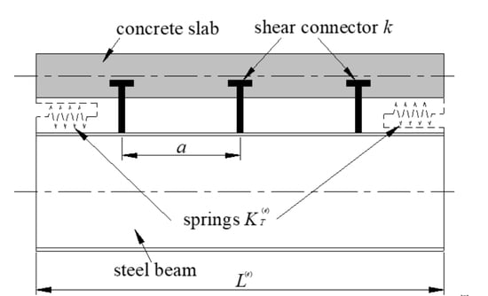
In the composite beam element model, the distance between any two adjacent shear connectors in a series that is uniformly arranged along the length of the element is generally not equal to the length of element. Therefore, it is essential to simplify the shear connectors of the composite beam element through the use of two springs, which are placed at the two ends of the element, respectively, as shown in Figure 1.

$$K_T^{(e)}=\frac{k·L^{(e)}}{2·a}$$

(1)

where k is the shear stiffness of a single shear connector, L^(e) is the length of the element model, and a is the distance between adjacent shear connectors.

2.3. Displacement and Strain Representation

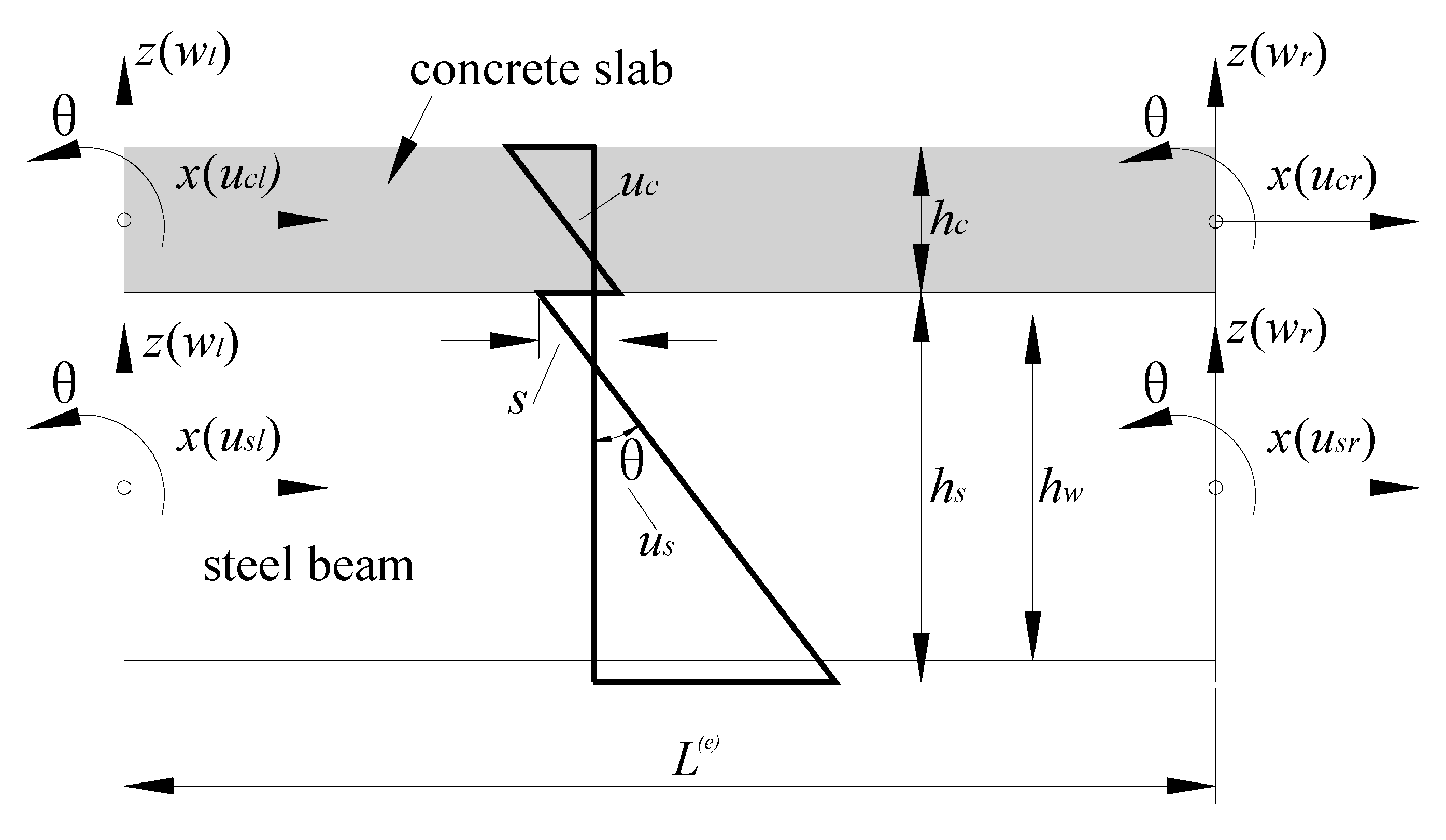
In terms of Assumption 3 in Section 2.1, both the concrete slab and the steel beam have the same transverse displacement w^(e) and normal rotation θ^(e) at each node of the element, but they could have different axial displacements. Consequently, longitudinal slip s^(e) exists at the interface between the concrete slab and the steel beam; however, interface slip s^(e) is relative to the axial displacement $\left[u_c^{(e)},u_s^{(e)}\right]$ and the rotation θ^(e). Therefore, the composite beam element model has 4 degrees of freedom at each node, i.e., $\left[u_c^{(e)},u_s^{(e)},w^{(e)},{\theta }^{(e)}\right]$. The displacement field of the composite beam element model is depicted in Figure 2.

Based on Figure 2, the expression of the nodal displacement vector of the composite beam element model can be presented as:

$${\mathit{a}}^{(e)}={\left[u_{cl}^{(e)},u_{sl}^{(e)},w_l^{(e)},{\theta }_l^{(e)},u_{cr}^{(e)},u_{sr}^{(e)},w_r^{(e)},{\theta }_r^{(e)}\right]}^T$$

(2)

in which the subscripts l and r represent the left node and the right node of the composite beam element, respectively.

As shown in Figure 2, the expression of the axial displacement ${\overline{u}}_c^{(e)}(x,z)$ at any point on the cross-section of the concrete slab can be written as

$${\overline{u}}_c^{(e)}(x,z)=u_c^{(e)}(x)-z_c·{\theta }^{(e)}(x)$$

(3)

Similarly, the expression of the axial displacement ${\overline{u}}_s^{(e)}(x,z)$ at any point on the cross-section of the steel beam can be written as

$${\overline{u}}_s^{(e)}(x,z)=u_s^{(e)}(x)-z_s·{\theta }^{(e)}(x)$$

(4)

At the same time, the interface slip s^(e) between the concrete slab and the steel beam of the composite beam element model can be expressed as

$$s^{(e)}={\left({\overline{u}}_c^{(e)}\right)}_{z_c=\frac{-h_c}{2}}-{\left({\overline{u}}_s^{(e)}\right)}_{z_s=\frac{h_s}{2}}=u_c^{(e)}-u_s^{(e)}+{\theta }^{(e)}·d$$

(5)

where d = (h_c + h_s)/2.

Therefore, the interface slip of the left node s_l^(e) and the interface slip of the right node s_r^(e) can be expressed as

$$s_l^{(e)}=u_{cl}^{(e)}-u_{sl}^{(e)}+{\theta }_l^{(e)}·d=\left[1,-1,0,d,0,0,0,0\right]·{\mathit{a}}^{(e)}={\left[{\mathit{B}}_{kl}^{(e)}\right]}^T·{\mathit{a}}^{(e)}$$

(6)

$$s_r^{(e)}=u_{cr}^{(e)}-u_{sr}^{(e)}+{\theta }_r^{(e)}·d=\left[0,0,0,0,1,-1,0,d\right]·{\mathit{a}}^{(e)}={\left[{\mathit{B}}_{kr}^{(e)}\right]}^T·{\mathit{a}}^{(e)}$$

(7)

where ${\left[{\mathit{B}}_{kl}^{(e)}\right]}^T$ and ${\left[{\mathit{B}}_{kr}^{(e)}\right]}^T$ are the slip-displacement matrices.

Generally, small deflection theory is employed, and then the strain-displacement relationships on the cross-section of the concrete slab and the steel beam can be written as,

$${\overline{\epsilon }}_c^{(e)}(x)=\frac{d{\overline{u}}_c^{(e)}}{dx}=\frac{d{u}_c^{(e)}}{dx}-z_c\frac{d{\theta }^{(e)}}{dx}=\frac{d{u}_c^{(e)}}{dx}-z_c\frac{d^2{w}^{(e)}}{d{x}^2}$$

(8)

$${\overline{\epsilon }}_s^{(e)}(x)=\frac{d{\overline{u}}_s^{(e)}}{dx}=\frac{d{u}_s^{(e)}}{dx}-z_s\frac{d{\theta }^{(e)}}{dx}=\frac{d{u}_s^{(e)}}{dx}-z_s\frac{d^2{w}^{(e)}}{d{x}^2}$$

(9)

In view of Assumption 1 in Section 2.1, it is reasonable to consider the two components of composite beams separately, as a Euler-Bernoulli beam. Employing the Euler-Bernoulli beam theory, it is reasonable to neglect the cross-sectional shear deformation. In this paper, the axial displacement $u_c^{(e)}$ or $u_s^{(e)}$ is interpolated by using the linear Lagrangian function, and the transversal displacement w is interpolated by using the cubic Hermitian interpolation function.

(1) Function of axial displacement

The axial displacement $u_c^{(e)}$ or $u_s^{(e)}$ (as shown in Figure 2) at any point along the length of the composite beam element can be expressed in a general form by adopting the dimensionless coordinate system as

$$u{(\xi )}^{(e)}=\left[N{(\xi )}_1^{(e)},N{(\xi )}_2^{(e)}\right]\left[\begin{array}{l}{u}_l^{(e)}\\ u_r^{(e)}\end{array}\right]$$

(10)

in which the shape function vector $\left[N{(\xi )}_1^{(e)},N{(\xi )}_2^{(e)}\right]=\left[1-\xi /2,1+\xi /2\right]$.

Therefore, the axial displacement $u_c^{(e)}$ or $u_s^{(e)}$ can be written as

$$\{\begin{array}{l}u{(\xi )}_c^{(e)}=\left[N{(\xi )}_1^{(e)},N{(\xi )}_2^{(e)}\right]{\left[u_{cl}^{(e)},u_{cr}^{(e)}\right]}^T\\ u{(\xi )}_s^{(e)}=\left[N{(\xi )}_1^{(e)},N{(\xi )}_2^{(e)}\right]{\left[u_{sl}^{(e)},u_{sr}^{(e)}\right]}^T\end{array}$$

(11)

The axial strain-displacement relationship can be represented as

$$\frac{d{u}^{(e)}(\xi )}{d\xi }=\left[{\left(\frac{d{N}_1}{d\xi }\right)}^{(e)},{\left(\frac{d{N}_2}{d\xi }\right)}^{(e)}\right]\left[\begin{array}{c}{u}_l^{(e)}\\ u_r^{(e)}\end{array}\right]=\left[-\frac{1}{2},\frac{1}{2}\right]\left[\begin{array}{c}{u}_l^{(e)}\\ u_r^{(e)}\end{array}\right]$$

(12)

and the relationship between absolute coordinates and relative coordinates is

$$\{\begin{array}{l}x=\frac{L^{(e)}}{2}(1+\xi )\\ dx=\frac{L^{(e)}}{2}d\xi \end{array}$$

(13)

Thus, the axial strain-displacement relationship for the concrete slab and the steel beam in absolute coordinates can be given as

$$\{\begin{array}{l}\frac{d{u}_c^{(e)}(x)}{dx}=\left[-\frac{1}{L^{(e)}},\frac{1}{L^{(e)}}\right]\left[\begin{array}{c}{u}_{cl}^{(e)}\\ u_{cr}^{(e)}\end{array}\right]\\ \frac{d{u}_s^{(e)}(x)}{dx}=\left[-\frac{1}{L^{(e)}},\frac{1}{L^{(e)}}\right]\left[\begin{array}{c}{u}_{sl}^{(e)}\\ u_{sr}^{(e)}\end{array}\right]\end{array}$$

(14)

(2) Function of deflection

The deflection $w^{(e)}(x)$ (as shown in Figure 2) at any point along the length of the composite beam element can be written by utilizing the dimensionless coordinate system as

$$w^{(e)}(\xi )={\left[N_{bi}^{(e)}(\xi )\right]}^T·{\mathit{a}}_b^{(e)}$$

(15)

in which

$${\mathit{a}}_b^{(e)}={\left[w_l^{(e)},{\theta }_l^{(e)},w_r^{(e)},{\theta }_r^{(e)}\right]}^T$$

(16)

$$N_{bi}^{(e)}(\xi )=\{\begin{array}{l}{N}_3^{(e)}(\xi )=(2-3\xi +{\xi }^3)/4\\ {\overline{N}}_3^{(e)}(\xi )=(1-\xi -{\xi }^2+{\xi }^3)/4\\ N_4^{(e)}(\xi )=(2+3\xi -{\xi }^3)/4\\ {\overline{N}}_4^{(e)}(\xi )=(-1-\xi +{\xi }^2+{\xi }^3)/4\end{array}$$

(17)

and the relationship between absolute coordinates and relative coordinates is

$${\left(\frac{d^{2}w}{d{x}^2}\right)}^{(e)}=\frac{4}{{\left(L^{(e)}\right)}^2}{\left(\frac{d^{2}w}{d{\xi }^2}\right)}^{(e)}$$

(18)

Thus, the curvature at any point along the length of the composite element can be written by using the coordinate transformation as

$$\begin{array}{l}\frac{d^2{w}^{(e)}}{d{x}^2}=\frac{4}{{\left(L^{(e)}\right)}^2}\left[\frac{d^2{N}_3^{(e)}}{d{x}^2},\frac{d^2{\overline{N}}_3^{(e)}}{d{x}^2}·\frac{L^{(e)}}{2},\frac{d^2{N}_4^{(e)}}{d{x}^2},\frac{d^2{\overline{N}}_4^{(e)}}{d{x}^2}·\frac{L^{(e)}}{2}\right]·{\mathit{a}}_b^{(e)}=\\ \left[\frac{6\xi }{{\left(L^{(e)}\right)}^2},\frac{-1+3\xi }{L^{(e)}},\frac{-6\xi }{{\left(L^{(e)}\right)}^2},\frac{1+3\xi }{L^{(e)}}\right]·{\mathit{a}}_b^{(e)}=\left[B_1^{(e)},B_2^{(e)},B_3^{(e)},B_4^{(e)}\right]·{\mathit{a}}_b^{(e)}={\left[{\mathit{B}}^{(e)}\right]}^T·{\mathit{a}}_b^{(e)}\end{array}$$

(19)

where ${\left[{\mathit{B}}^{(e)}\right]}^T$ is the longitudinal curvature-displacement matrix.

Thus, the axial strain at any point of cross-section of the concrete slab ${\overline{\epsilon }}_c^{(e)}$ can be written by substituting Equations (14) and (19) into Equation (8) as

$$\begin{array}{l}{\epsilon }_c^{(e)}(x)=\frac{d{\overline{u}}_c^{(e)}(x)}{dx}=\frac{d{u}_c^{(e)}}{dx}-z_c\frac{d^2{w}^{(e)}}{d{x}^2}=\\ \left[-\frac{1}{L^{(e)}},0,z_c\frac{-6\xi }{{\left(L^{(e)}\right)}^2},z_c\frac{1-3\xi }{L^{(e)}},\frac{1}{L^{(e)}},0,z_c\frac{6\xi }{{\left(L^{(e)}\right)}^2},z_c\frac{-1-3\xi }{L^{(e)}}\right]·{\mathit{a}}^{(e)}\\ ={\left[{\mathit{B}}_c^{(e)}\right]}^T·{\mathit{a}}^{(e)}\end{array}$$

(20)

where ${\left[{\mathit{B}}_c^{(e)}\right]}^T$ is the axial strain-displacement matrix for concrete slab.

Similarly, the axial strains at any point of the cross-section of the steel beam ${\overline{\epsilon }}_s^{(e)}$ can be obtained by substituting Equations (14) and (19) into Equation (9) as

$$\begin{array}{l}{\epsilon }_s^{(e)}(x)=\frac{d{\overline{u}}_s^{(e)}(x)}{dx}=\frac{d{u}_s^{(e)}}{dx}-z_s\frac{d{\theta }^{(e)}}{dx}=\\ \left[0,-\frac{1}{L^{(e)}},z_s\frac{-6\xi }{{\left(L^{(e)}\right)}^2},z_s\frac{1-3\xi }{L^{(e)}},0,\frac{1}{L^{(e)}},z_s\frac{6\xi }{{\left(L^{(e)}\right)}^2},z_s\frac{-1-3\xi }{L^{(e)}}\right]·{\mathit{a}}^{(e)}\\ ={\left[{\mathit{B}}_s^{(e)}\right]}^T·{\mathit{a}}^{(e)}\end{array}$$

(21)

where ${\left[{\mathit{B}}_s^{(e)}\right]}^T$ is the axial strain-displacement matrix for the steel beam.

2.4. Composite Beam Element Stiffness Matrix Evaluation

When a composite beam of length L is subjected to a uniformly distributed load q, the contribution to the total potential energy I from element (e) of length L^(e) can be expressed as

$$I^{(e)}=I_c^{(e)}+I_s^{(e)}+I_k^{(e)}-{\displaystyle {\int }_{L^{(e)}}{q}^{(e)}{w}^{(e)}dx}$$

(22)

where

$$\{\begin{array}{l}{I}_c^{(e)}=\frac{1}{2}{\displaystyle {\int }_{v{c}^{(e)}}{\sigma }_c^{(e)}{\epsilon }_c^{(e)}·dv}\\ I_s^{(e)}=\frac{1}{2}{\displaystyle {\int }_{v{s}^{(e)}}{\sigma }_s^{(e)}{\epsilon }_s^{(e)}·dv}\\ I_k^{(e)}=\frac{1}{2}{K}_T^{(e)}·{s_l^{(e)}}^2+\frac{1}{2}{K}_T^{(e)}·{s_r^{(e)}}^2\end{array}$$

(23)

The stress-strain relationships for an isotropic elastic material and the load-displacement relationships, using Hooke’s law to represent the springs, can be written as

$$\{\begin{array}{l}{\sigma }_c=E_c{\epsilon }_c\\ {\sigma }_s=E_s{\epsilon }_s\\ T_{Kl}=K_T^{(e)}{s}_l\\ T_{Kr}=K_T^{(e)}{s}_r\end{array}$$

(24)

Substituting Equations (1), (6), (7), (20), (21) and (24) into Equation (22), the total potential energy equation for element (e) can also be written as

$$\begin{array}{l}{I}^{(e)}=\frac{1}{2}{\displaystyle {\int }_{v{c}^{(e)}}{E}_c{{\epsilon }_c^{(e)}}^2·dv}+\frac{1}{2}{\displaystyle {\int }_{v{s}^{(e)}}{E}_s{{\epsilon }_s^{(e)}}^2·dv}+\frac{1}{2}{K}_T^{(e)}·{s_l^{(e)}}^2+\frac{1}{2}{K}_T^{(e)}·{s_r^{(e)}}^2-{\displaystyle {\int }_{L^{(e)}}q·w^{(e)}·dx}\\ =\frac{1}{2}{\displaystyle {\int }_{v{c}^{(e)}}{\left[{\mathit{a}}^{(e)}\right]}^T\left[{\mathit{B}}_c^{(e)}\right]E_c{\left[{\mathit{B}}_c^{(e)}\right]}^T{\mathit{a}}^{(e)}·dv}+\frac{1}{2}{\displaystyle {\int }_{v{s}^{(e)}}{\left[{\mathit{a}}^{(e)}\right]}^T\left[{\mathit{B}}_s^{(e)}\right]E_s{\left[{\mathit{B}}_s^{(e)}\right]}^T{\mathit{a}}^{(e)}·dv}+\\ \frac{1}{2}{\left[{\mathit{a}}^{(e)}\right]}^T\left[{\mathit{B}}_{kl}^{(e)}\right]K_T^{(e)}{\left[{\mathit{B}}_{kl}^{(e)}\right]}^T{\mathit{a}}^{(e)}+\frac{1}{2}{\left[{\mathit{a}}^{(e)}\right]}^T\left[{\mathit{B}}_{kr}^{(e)}\right]K_T^{(e)}{\left[{\mathit{B}}_{kr}^{(e)}\right]}^T{\mathit{a}}^{(e)}-{\displaystyle {\int }_{-1}^1\left[{\mathit{B}}_b^{(e)}\right]·q\frac{L^{(e)}}{2}d\xi }\\ =\frac{1}{2}{\left[{\mathit{a}}^{(e)}\right]}^T{\mathit{K}}_c^{(e)}{\mathit{a}}^{(e)}+\frac{1}{2}{\left[{\mathit{a}}^{(e)}\right]}^T{\mathit{K}}_s^{(e)}{\mathit{a}}^{(e)}+\frac{1}{2}{\left[{\mathit{a}}^{(e)}\right]}^T{\mathit{K}}_{Tl}^{(e)}{\mathit{a}}^{(e)}+\frac{1}{2}{\left[{\mathit{a}}^{(e)}\right]}^T{\mathit{K}}_{Tr}^{(e)}{\mathit{a}}^{(e)}-{\displaystyle {\int }_{-1}^1\left[{\mathit{B}}_b^{(e)}\right]·q\frac{L^{(e)}}{2}d\xi }\\ =\frac{1}{2}{\left[{\mathit{a}}^{(e)}\right]}^T{\mathit{K}}^{(e)}{\mathit{a}}^{(e)}-\mathit{f}\end{array}$$

(25)

in which

$$\begin{array}{l}{\mathit{K}}^{(e)}={\mathit{K}}_c^{(e)}+{\mathit{K}}_s^{(e)}+{\mathit{K}}_{Tl}^{(e)}+{\mathit{K}}_{Tr}^{(e)}\\ \left\{{\mathit{B}}_b^{(e)}\right\}={\left[0,0,N_3^{(e)}(\xi ),{\overline{N}}_3^{(e)}(\xi ),0,0,N_4^{(e)}(\xi ),{\overline{N}}_4^{(e)}(\xi )\right]}^T\\ {\mathit{K}}_c^{(e)}={\displaystyle {\int }_{-1}^1\left[{\mathit{B}}_c^{(e)}\right]·{\left(EA\right)}_c^{(e)}·{\left[{\mathit{B}}_c^{(e)}\right]}^T\frac{L^{(e)}}{2}d\xi }\\ {\mathit{K}}_s^{(e)}={\displaystyle {\int }_{-1}^1\left[{\mathit{B}}_s^{(e)}\right]·{\left(EA\right)}_s^{(e)}·{\left[{\mathit{B}}_s^{(e)}\right]}^T\frac{L^{(e)}}{2}d\xi }\\ {\mathit{K}}_{Tl}^{(e)}=\left[{\mathit{B}}_{kl}^{(e)}\right]·K_T^{(e)}·{\left[{\mathit{B}}_{kl}^{(e)}\right]}^T\\ {\mathit{K}}_{Tr}^{(e)}=\left[{\mathit{B}}_{kr}^{(e)}\right]·K_T^{(e)}·{\left[{\mathit{B}}_{kr}^{(e)}\right]}^T\\ \mathit{f}={\displaystyle {\int }_{-1}^1\left[{\mathit{B}}_b^{(e)}\right]·q\frac{L^{(e)}}{2}d\xi }\end{array}$$

(26)

Therefore, the element stiffness matrix ${\mathit{K}}^{(e)}$[8×8] for a composite beam element can be written in a symmetric form as follows

$$\left[\begin{array}{cccccccc}\frac{{(EA)}_{\mathrm{c}}^{(e)}}{L^{(e)}}+K_{\mathrm{T}}^{(e)}& -K_{\mathrm{T}}^{(e)}& 0& \frac{-{(ES)}_{\mathrm{c}}^{(e)}}{L^{(e)}}+K_{\mathrm{T}}^{(e)}d& -\frac{{(EA)}_c^{(e)}}{L^{(e)}}& 0& 0& \frac{{(ES)}_c^{(e)}}{L^{(e)}}\\ & \frac{{(EA)}_{\mathrm{s}}^{(e)}}{L^{(e)}}+K_{\mathrm{T}}^{(e)}& 0& \frac{-{(ES)}_{\mathrm{s}}^{(e)}}{L^{(e)}}-K_{\mathrm{T}}^{(e)}d& 0& -\frac{{(EA)}_s^{(e)}}{L^{(e)}}& 0& \frac{{(ES)}_s^{(e)}}{L^{(e)}}\\ & & \frac{12{(EI)}_{\mathrm{c}}^{(e)}}{L^{(e)}{}^3}+\frac{12{(EI)}_{\mathrm{s}}^{(e)}}{L^{(e)}{}^3}& \frac{6{(EI)}_{\mathrm{c}}^{(e)}}{L^{(e)}{}^2}+\frac{6{(EI)}_{\mathrm{s}}^{(e)}}{L^{(e)}{}^2}& 0& 0& -\frac{12{(EI)}_{\mathrm{c}}^{(e)}}{L^{(e)}{}^3}-\frac{12{(EI)}_{\mathrm{s}}^{(e)}}{L^{(e)}{}^3}& \frac{6{(EI)}_{\mathrm{c}}^{(e)}}{L^{(e)}{}^2}+\frac{6{(EI)}_{\mathrm{s}}^{(e)}}{L^{(e)}{}^2}\\ & & & \frac{4{(EI)}_{\mathrm{c}}^{(e)}}{L^{(e)}}+\frac{4{(EI)}_{\mathrm{s}}^{(e)}}{L^{(e)}}+K_{\mathrm{T}}^{(e)}{d}^2& \frac{{(ES)}_c^{(e)}}{L^{(e)}}& \frac{{(ES)}_s^{(e)}}{L^{(e)}}& \frac{6{(EI)}_{\mathrm{c}}^{(e)}}{L^{(e)}{}^2}-\frac{6{(EI)}_{\mathrm{s}}^{(e)}}{L^{(e)}{}^2}& \frac{2{(EI)}_{\mathrm{c}}^{(e)}}{L^{(e)}}+\frac{2{(EI)}_{\mathrm{s}}^{(e)}}{L^{(e)}}\\ & & & & \frac{{(EA)}_{\mathrm{c}}^{(e)}}{L^{(e)}}+K_{\mathrm{T}}^{(e)}& -K_{\mathrm{T}}^{(e)}& 0& \frac{-{(ES)}_c^{(e)}}{L^{(e)}}+K_{\mathrm{T}}^{(e)}d\\ & & \mathrm{symmetric}& & & \frac{{(EA)}_{\mathrm{s}}^{(e)}}{L^{(e)}}+K_{\mathrm{T}}^{(e)}& 0& \frac{-{(ES)}_s^{(e)}}{L^{(e)}}-K_{\mathrm{T}}^{(e)}d\\ & & & & & & \frac{12{(EI)}_{\mathrm{c}}^{(e)}}{L^{(e)}{}^3}+\frac{12{(EI)}_{\mathrm{s}}^{(e)}}{L^{(e)}{}^3}& -\frac{6{(EI)}_{\mathrm{c}}^{(\mathrm{e})}}{L^{(e)}{}^2}-\frac{6{(EI)}_{\mathrm{s}}^{(e)}}{L^{(e)}{}^2}\\ & & & & & & & \frac{4{(EI)}_{\mathrm{c}}^{(e)}}{L^{(e)}}+\frac{4{(EI)}_{\mathrm{s}}^{(e)}}{L^{(e)}}+K_{\mathrm{T}}^{(e)}{d}^2\end{array}\right]$$

(27)

3. Validation of the Composite Beam Element Model

In this section, a finite element program is developed on the basis of the element stiffness matrix of the proposed composite beam element model that was established in the above section.

The developed element is verified by comparing it against previous experimental data [22,23], and also against the closed-form solution [24].

3.1. Comparison with Experimental Results

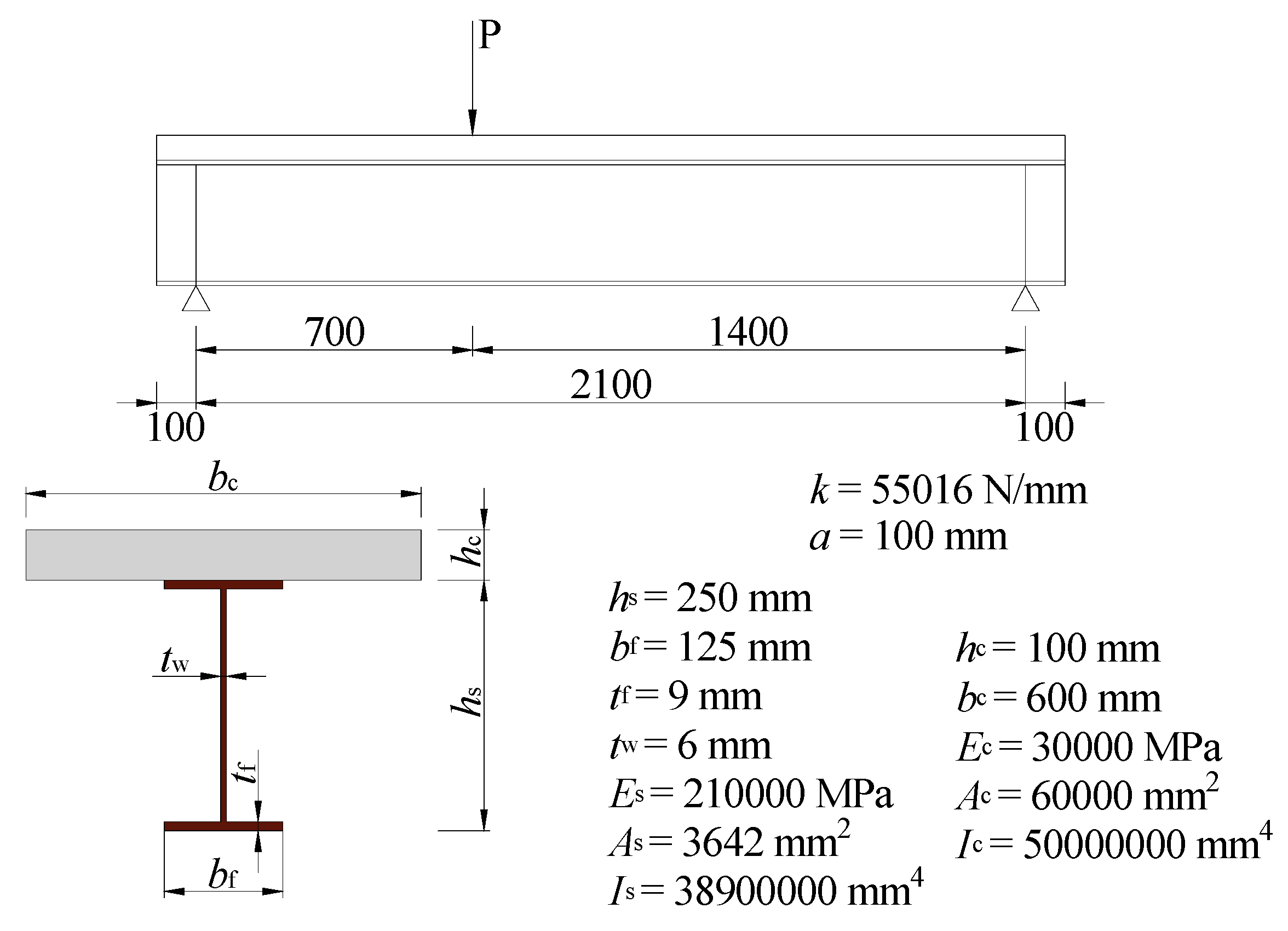
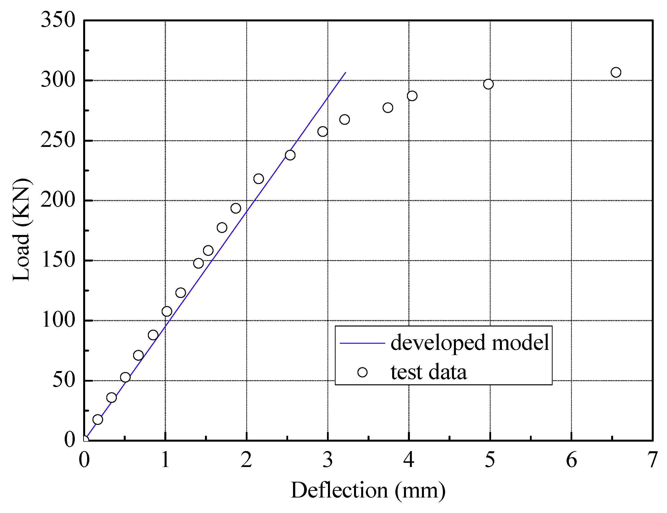
In this section, the developed composite beam element model is employed to calculate the maximum deflection of the simply supported composite beam employed by Wang et al. [22,23], and the numerical results are compared with the corresponding experimental results. In the simulation, the simply supported composite beam is modeled using twenty-one elements. The geometric characteristics and the material properties of the simply supported beam with uniformly distributed shear connectors are shown in Figure 3. The comparison between the load-deflection curve of the numerical results and that of the experimental results is shown in Figure 4. In Figure 4, a good agreement can be observed between the numerical results and the experimental data in the elastic stage. However, the cross-section enters an elastic-plastic state when the applied load is greater than 250kN, and the difference between the numerical results and the experimental data becomes greater and greater. In other words, the proposed element model is not applicable to the final stage of loading.

3.2. Comparison with the Closed-Form Solutions

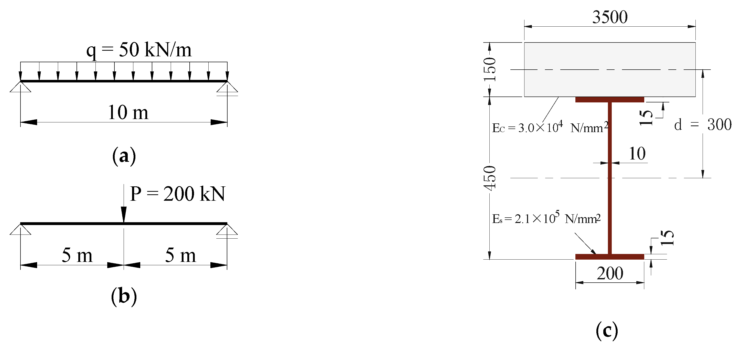
For the sake of demonstrating that the developed element model can be used to simulate composite beams with both full and partial interaction, the deflection and interface slip are analyzed for a simply supported composite beam with a shear connector distance a of 250 mm by using the composite beam element. A comparison is made between the results obtained using the developed element model and values of existing closed-form solutions [24]. To obtain as many results as possible for the deflection and the interface slip on the composite beam in order to compare them with the results of the closed-form solutions, the beam is modeled using twenty elements. The same simply supported composite beam is analyzed under two different loads (a uniformly distributed load and a point load). The applied loads on the composite beam, the sectional size, and the corresponding elastic material parameters can be seen in Figure 5. Furthermore, a simply supported composite beam have different values for the stiffness of shear connector k is considered in the comparison, and full interaction is reached when k is 1.0 × 10⁸ N/mm. The corresponding results obtained, as well as the related parameters, are shown in

Table 1. Comparison of maximum deflection and the interface slip of the beam end for two types of load.

	q = 50N/mm, a = 250mm						P = 200KN, a = 250mm
	k = 3.46 × 104 N/mm		k = 1.0 × 105 N/mm		k = 1.0 × 108 N/mm		k = 3.46 × 104 N/mm		k = 1.0 × 105 N/mm		k = 1.0 × 108 N/mm
	w	s	w	s	w	s	w	s	w	s	w	s
Numerial result (mm)	−37.26	2.10	−29.86	0.95	−24.04	0.00	−24.08	1.18	−19.34	0.50	−15.40	0.00
Closed result (mm)	−37.24	2.10	−29.80	0.95	−23.96	0.00	−24.06	1.18	−19.30	0.50	−15.33	0.00
Relative error (%)	0.05	0	0.20	0	0.33	0	0.08	0.14	0.21	0	0.46	0

.

It can be found from Table 1 that, for different types of load and shear connection degrees, the maximum absolute value of relative error is only 0.46%, indicating a good agreement. This indicates that the results calculated by the proposed element model are close to those of the closed-form solutions; therefore, the proposed element model is sufficiently accurate and stable for the numerical analysis of composite beams.

It can also be found that, with regard to both the evenly distributed load case and the point load case, (1) the maximum deflections occur at the mid-span of the beams, and the values of deflection decrease with increasing values of shear connector stiffness; and (2) the maximum interface slips take place at the end of beams; moreover, the slip values increase with decreasing values of shear connector stiffness. This is because of the degree of shear connection, whereby shear connectors with a high degree of connector stiffness are able to resist interface slip and deflection very well. From Table 1, it can be observed that full interaction is achieved between the two components of the composite beam when the stiffness value of a shear connector k reaches 1.0e8 N/mm. The comparison of maximum deflection between partial interaction and full interaction for the two types of load can be seen in

Table 2. Comparison of maximum deflection between partial connection and full connection for the composite beam.

Load Types	k=3.46 × 104 N/mm w1 (mm)	k=1.0 × 108 N/mm w2 (mm)	(w1 − w2)/w1 (%)
Uniformly distributed	−37.26	−24.08	35.37
Point	−24.04	−15.40	35.94

.

As shown in Table 2, when the value of connector stiffness increases from 3.46e4 N/mm to 1.0e8 N/mm, i.e., from partial interaction to full interaction, the maximum deflection at the mid-span of the beam decreases by 35.37% or so in the case of a uniformly distributed load; meanwhile, the maximum deflection decreases by as much as 35.94% in the point load case. In addition, it can be seen that the deflection and interface slip of the composite beam decreases with increasing values of stiffness of a shear connector k for the same composite beam. On the other hand, slip exists at the interface between the two components of the composite beams because of the partial interaction, thus affecting the deformation capacity of the composite beam. Therefore, interface slip has a great influence on deflection. Nevertheless, a great number of composite beams employ partial interaction, since slip always exists at the interface between the concrete slab and the steel beam of a composite beam. As a consequence, it is unsafe to ignore the existing interface slip of a composite beam with partial interaction; in other words, interface slip should be considered in deflection analysis.

4. Optimal Layout for Shear Connectors

4.1. Uniformly Distributed Shear Connectors

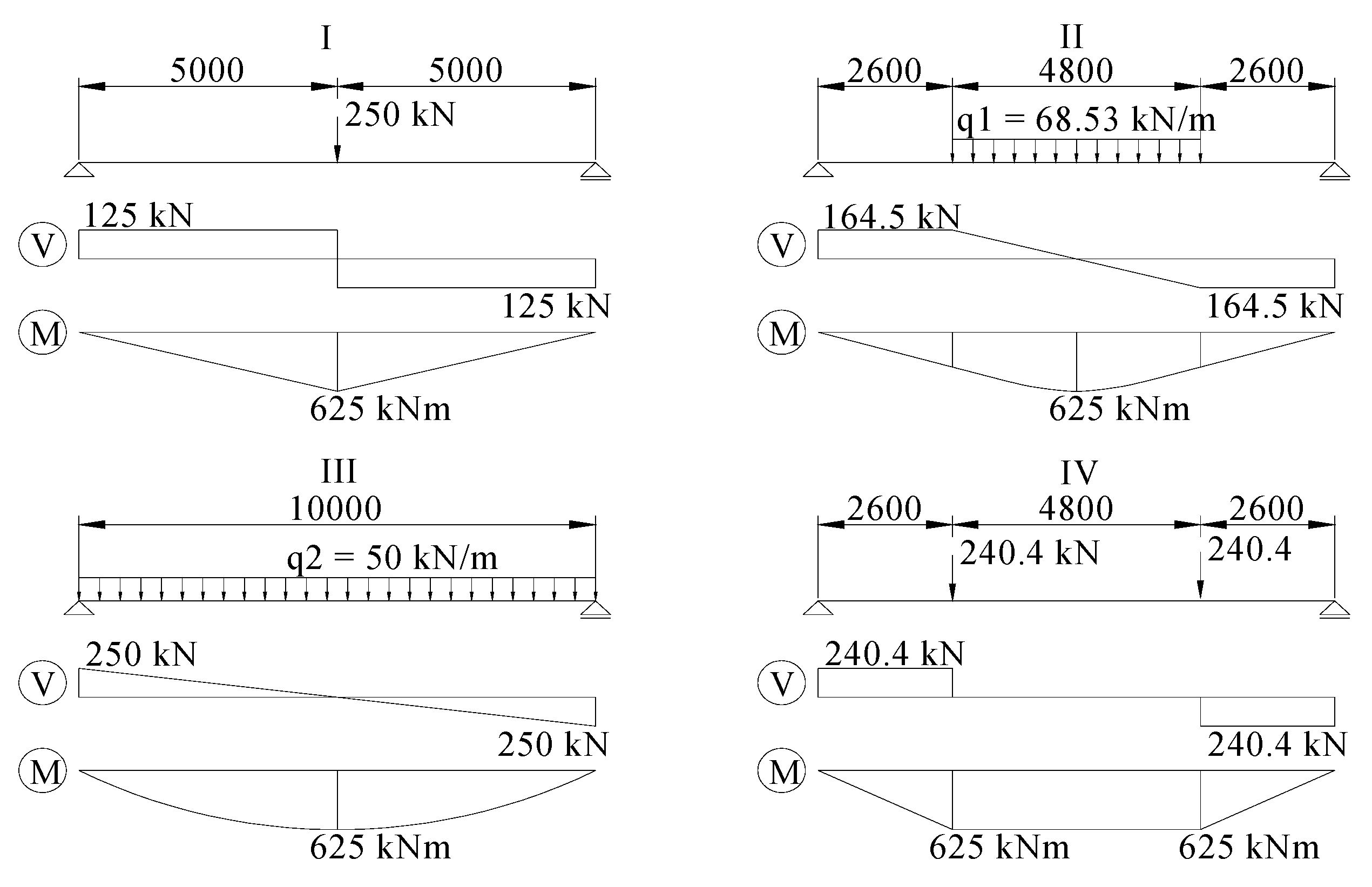
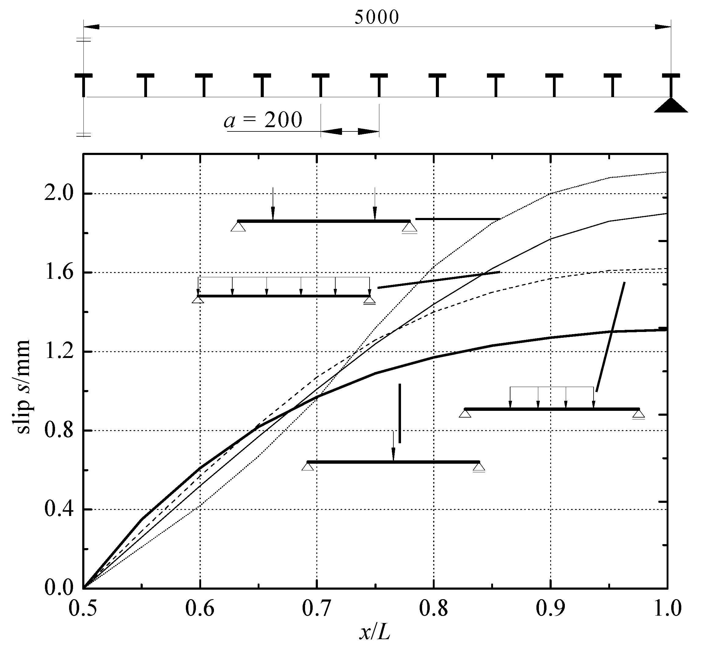
In most of practical composite beams, the shear connectors are uniformly distributed along the beam, since this type of distribution reduces the interface slip to some extent, and it is also convenient to construct. To reveal the disadvantages of this approach, a composite beam with uniformly distributed shear connectors is investigated with regard to the distribution of the interface slip along the longitudinal direction of beam. Four different types of load (as shown in Figure 6) are applied to a simply supported composite beam with partial interaction, i.e., stiffness of shear connector k = 3.46 × 10⁴ N/mm and connector distance a = 200 mm. The shear force diagrams of the four load cases are shown in Figure 6, and the cross-section size and material parameters of the composite beam are the same as those given in Figure 5. Because it is symmetrical, only one-half of the composite beam is studied, and the results for the interface slip of the half-span beam under four different load cases are depicted in Figure 7.

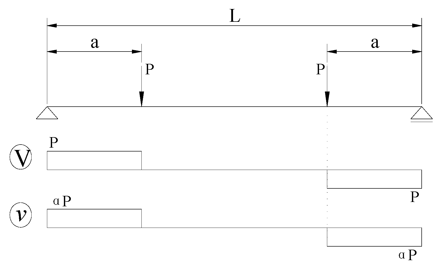
As can be observed in Figure 6, the distribution of the cross-sectional shear force along the beam becomes increasingly uneven from the first type of load to the fourth type of load. It is known from Liu [25] that the distribution of shear flow v at the interface is the same as the distribution of cross-sectional shear force V along the beam in terms of ν = VS_z/I_z, as shown in Figure 8, in which α = S_z/I_z is a constant value for a given cross-section. Meanwhile, according to Assumption 5 in Section 2.1, the distribution of interface slip is similar to the distribution of shear flow at the interface. Thus, the distribution of interface slip is similar to the distribution of cross-sectional shear force. For this reason, with the increasingly uneven distribution of cross-sectional shear force along the beam from the first type of load to the fourth type of load, a more uneven distribution of interface slip occurs, as can be seen in Figure 7. For example, the fourth type of load (in Figure 6) is an extreme case, in which the maximum cross-sectional shear force occurs at the two ends of the beam and the cross-sectional shear force is at its minimum at mid-span. Correspondingly, the distribution of interface slip is the most uneven, as shown in Figure 7 and

Table 3. Comparison of maximum slip at the end of the beam under four load cases.

Load Types	I	II	III	IV
Maximum slip smax (mm)	1.31	1.62	1.90	2.11
smax/smaxI	1.0	1.24	1.45	1.61

. Essentially, the role of the shear connectors is to resist interface slip. Therefore, for cases of uneven distribution of shear force, the number of shear connectors in the mid-span region is too great to be utilized fully, while the number of shear connectors in the region of the supports is not sufficient to resist the interface slip. Nevertheless, the shear force varies along the beam for most load cases. Therefore, uniform distribution may not be the best way to distribute shear connectors.

4.2. Stepwise Uniform Distribution for Shear Connectors

As can be seen from the above section, the uniform distribution of shear connectors has its own disadvantages. The stiffness of the shear connectors in the mid-span region is not being fully utilized to reduce interface slip. However, interface slip has a significant influence on deflection, as described in Section 3, so it is increasingly important to reduce interface slip in order to improve the composite action and reduce the deflection of composite beams. It was made known by Wang and Dong [8] that the distribution of interface slip is directly related to the distribution of shear connector density. Although the beam can effectively reduce the interface slip under a triangular distribution of shear connector density [8], such a distribution of shear connectors is inconvenient for engineering applications, since each connector has a different stiffness along the half-span. As can be observed in Table 1, the interface slip along the beam is equal to zero when the two components of the composite beam achieve full interaction. Therefore, the most direct and effective way to reduce the interface slip of composite beams with partial interaction is to increase the stiffness of shear connectors in the regions with the largest interface slip. For the purpose of achieving this goal, there are three different ways of increasing the stiffness: (1) an increase in the number of shear connectors; (2) an increase in the stiffness value of every shear connector; and (3) adopting a stepwise uniform distribution for shear connectors without increasing the total number of shear connectors. The first two methods have their own deficiencies, not only with regard to the stiffness of shear connectors being incompletely utilized at the mid-span, but also with respect to the increase of cost. Furthermore, it is increasingly difficult to accommodate the shear connectors in the beam when the total number of shear connectors increases. Therefore, this paper will adopt the third method for the developed composite beam element, which is to rearrange the shear connectors to achieve an optimal layout without increasing the total number of shear connectors. The optimal layout method adopts a stepwise uniform distribution of shear connectors—namely, 2-stepped rectangles, 3-stepped rectangles and 5-stepped rectangles (as shown in Figure 9)—to approximate the triangular distribution of shear connector density along the beam [6]. For the purpose of effectively utilizing the shear connectors and reducing the interface slip, a greater number of shear connectors are distributed in the region of the beam ends, and a lower number of shear connectors are distributed in the mid-span region. Meanwhile, the total number of shear connectors is assumed to remain constant before and after redistribution. The efficiency of the proposed connector layout method is evaluated by comparing the interface slip before and after the redistribution. The comparison is performed on a simply supported composite beam with partial interaction, i.e., with the stiffness value of a shear connector k = 3.46 × 10⁴ N/mm. The loads applied on the composite beam are shown in Figure 6, and the cross-sectional size and corresponding elastic material parameters are the same as those shown in Figure 5. Figure 9 shows the redistribution of the shear connectors along the composite beam, which is divided into 20 elements based on a distribution using different stepped rectangles. The slip distribution curves obtained by using different types of distribution for the shear connectors are compared in Figure 10a–d. The corresponding slips of the composite beam end are shown in

Table 4. Comparison of beam end interface slip under four load cases.

Load Types	I	II	III	IV
Uniformly slip s1 (mm)	1.31	1.62	1.90	2.11
2-stepped rectangles slip s2 (mm)	1.12	1.40	1.63	1.83
3-stepped rectangles slip s3 (mm)	1.02	1.27	1.49	1.66
5-stepped rectangles slip s4 (mm)	0.94	1.17	1.37	1.52
(s1 − s2)/ s1 (%)	14.17	13.33	13.95	13.47
(s1 − s3)/ s1 (%)	21.59	21.48	21.33	21.53
(s1 − s4)/ s1 (%)	27.96	27.96	27.65	28.02

.

It can be observed from Figure 10a–d and Table 4 that, with an increase in the number of stepped rectangles, the interface slip of the beam end decreases. When adopting a 2-stepped rectangle distribution, the interface slip of the beam end decreases by 14.17% for the four kinds of load, while the interface slip decreases by 21.59% for the 3-stepped rectangle distribution, and the interface slip decreases drastically, by 28.02%, for the 5-stepped rectangle distribution. Nevertheless, it can be clearly seen from Figure 10a that the location at which maximum interface slip occurs gradually moves from the beam end toward the mid-span when using the 5-stepped rectangle distribution method, and this phenomenon is also apparent in Figure 10b. The main reason for this is that cross-sectional shear force is uniformly distributed along the composite beams for the first type of load and is relatively evenly distributed along the beam for the second type of load; but compared with the 3-stepped rectangle distribution, the 5-stepped rectangle distribution results in several too many shear connectors concentrated at the two ends of the beam. In this way, the number of shear connectors in the region close to the mid-span is too small to resist interface slip, leading to the movement of the maximum interface slip from either end of the beam towards the mid-span. However, the 3-stepped rectangle distribution facilitates application in practice, because this type of distribution has fewer segments than the 5-stepped rectangle distribution, and, most importantly, the 3-stepped rectangle distribution method is able to effectively decrease the interface slip. For these reasons, it is reasonable to select the 3-stepped rectangle distribution method as an optimal layout method for the stepwise uniform distribution of shear connectors.

4.3. Effect of Shear Connector Distribution on Deflection

As described in Section 3, the deflection of composite beams decreases with the decrease in interface slip. From Section 4.2, we can get that the interface slip is decreased by using different redistributions of shear connectors. The corresponding maximum deflections along the beam under different stepped rectangle distributions of shear connectors (as shown in Figure 9) are shown in

Table 5. Comparison of maximum deflection under four load cases.

Load Types	I	II	III	IV
Uniformly deflection w1 (mm)	−31.35	−36.54	−38.75	−41.75
2-stepped rectangles deflection w2 (mm)	−30.56	−35.84	−37.51	−40.67
3-stepped rectangles deflection w3 (mm)	−30.17	−35.10	−36.92	−39.71
5-stepped rectangles deflection w4 (mm)	−29.87	−34.66	−36.43	−39.10
(w1 − w2)/w1 (%)	2.51	1.93	3.18	2.57
(w1 − w3)/w1 (%)	3.75	3.95	4.72	4.88

. As shown in Table 5, the 2-stepped rectangle distribution method can reduce the maximum deflection along the beam by 3.18% for the four kinds of load. Meanwhile, the 3-stepped rectangle distribution method is able to reduce the maximum deflection by 4.88%, and the 5-stepped rectangle distribution method is able to reduce the maximum deflection by 6.35%. However, it is not necessary to increase the total number of shear connectors. In other words, the proposed connector layout method can enlarge the service space without increasing the construction cost; furthermore, it can decrease the interface slip and deflection of composite beams, and increase the composite effect and stiffness of composite beams.

5. Conclusions

This paper proposes an optimal layout method of shear connectors for a steel-concrete composite beam with interface slip that is based on a one-dimensional composite beam element model. The proposed composite beam element model consists of two beam components, which are considered to be a Euler-Bernoulli beam, and the corresponding element stiffness matrix is derived by adopting the total potential energy method. After the efficiency of the developed element is validated by comparisons with experimental data and closed-form solutions, we arrive at an optimal layout method for the uniform distribution of shear connectors based on the developed element. The main conclusions drawn from this study can be summarized as follows:

(1) The proposed composite beam element model is a unified formulation and is applicable to any complex load conditions, particularly cases with an arbitrary stiffness and arbitrary distribution of shear connectors. The results obtained using the developed program are in good agreement with experimental data in the elastic stage, and are also in good agreement with those of closed-form solutions.

(2) Compared to the uniform distribution method, the proposed connector layout method can effectively decrease the interface slip and deflection of composite beams and increase the composite effect and stiffness without increasing the number of shear connectors.

(3) Based on the developed composite beam element model, the proposed connector layout method can be applied under arbitrary load conditions, and the type of distribution does not need to be determined afresh for different load cases.

(4) The 3-stepped rectangle distribution method is an optimal layout for the shear connectors of composite beams, since the distribution type of the shear connectors can not only decrease the interface slip and deflection, but will also clearly never result in the locations at which maximum interface slip occurs moving from the beam ends toward the mid-span.

However, the developed composite element model was verified only by using the experimental data and closed-form solutions provided in the paper, and the proposed connector layout method is applied to a simply supported beam. In the future, further numerical simulations and experimental research need to be conducted to verify the developed element model and to confirm the efficiency of the proposed connector layout method.

References

- Naser, M.Z.; Kodur, V.K.R. Comparative fire behavior of composite girders under flexural and shear loading. Thin-Walled Struct. 2017, 116, 82–90. [Google Scholar] [CrossRef]
- Bradford, M.A.; Gilbert, R.I. Time-dependent behavior of simply-supported steel-concrete composite beams. Mag. Concr. Res. 1991, 43, 265–274. [Google Scholar] [CrossRef]
- Lai, Z.C.; Varma, A.H.; Griffis, L.G. Analysis and design of noncompact and slender CFT beam-columns. ASCE J. Struct. Eng. 2016, 142, 04015097. [Google Scholar] [CrossRef]
- Nie, J.G.; Li, Y.; Yu, Z.W.; Chen, Y.Y. Study on short and long-term rigidity of composite steel-concrete beams. J. Tsinghua Univ. (Sci. & Technol.) 1998, 38, 38–41. (In Chinese) [Google Scholar]
- Nie, J.; Cai, C.S. Steel-concrete composite beams considering shear slip effects. J. Struct. Eng. 2003, 129, 495–506. [Google Scholar] [CrossRef]
- Grant, J.A.; Fisher, J.W.; Slutter, R.G. Composite beams with formed steel deck. Eng. J. 1977, 12, 24–43. [Google Scholar]
- Jasim, N.A. Deflections of partially composite beams with linear connector density. J. Constr. Steel Res. 1999, 49, 241–254. [Google Scholar] [CrossRef]
- Wang, G.N.; Dong, W.W. Calculation of interlayer slip for composite beams after optimization of shear connectors. Low Temp. Arch. Technol. 2012, 34, 30–32. [Google Scholar]
- Wang, P.; Zhou, D.H.; Wang, Y.H.; Wang, H.T. Calculation on slip of composite beams with stepwise uniform distribution of shear connectors. Build. Struct. 2011, 41, 96–101. (In Chinese) [Google Scholar]
- Han, J.H.; Hoa, S.V. A three-dimensional multilayer composite finite element for stress analysis of composite laminates. Int. J. Numer. Methods Eng. 1993, 36, 3903–3914. [Google Scholar] [CrossRef]
- Ferreira, A.J.M.; Camanho, P.P.; Marques, A.T.; Fernandes, A.A. Modelling of concrete beams reinforced with FRP re-bars. Compos. Struct. 2001, 53, 107–116. [Google Scholar] [CrossRef]
- Yu, H. A higher-order finite element for analysis of composite laminated structures. Compos. Struct. 1994, 28, 375–383. [Google Scholar] [CrossRef]
- Surana, K.S.; Nguyen, S.H. Two-dimensional curved beam element with higher-order hierarchical transverse approximation for laminated composites. Compos. Struct. 1990, 36, 499–511. [Google Scholar] [CrossRef]
- Manjunatha, B.S.; Kant, T. New theories for symmetric/unsymmetric composite and sandwich beams with C0 finite elements. Compos. Struct. 1993, 23, 61–73. [Google Scholar] [CrossRef]
- Neto, M.A.; Yu, W.; Roy, S. Two finite elements for general composite beam with piezoelectric actuators and sensors. Finite Elem. Anal. Des. 2009, 45, 295–304. [Google Scholar] [CrossRef]
- Aribert, J.M.; Xu, H.; Ragneau, E. Theoretical investigation of moment redistribution in composite continuous beams of different classes. In Composite Construction in Steel and Concrete III; American Society of Civil Engineers: New York, NY, USA, 1996; pp. 392–405. [Google Scholar]
- El-Lobody, E.; Lam, D. Finite element analysis of steel-concrete composite girders. Adv. Struct. Eng. 2003, 6, 267–281. [Google Scholar] [CrossRef]
- Ranzi, G.; Bradford, M.A.; Uy, B. A direct stiffness analysis of a composite beam with partial interaction. Int. J. Numer. Methods Eng. 2004, 61, 657–672. [Google Scholar] [CrossRef]
- Lin, X.; Zhang, Y.X. A novel one-dimensional two-node shear-flexible layered composite beam element. Finite Elem. Anal. Des. 2011, 47, 676–682. [Google Scholar] [CrossRef]
- Nie, J.G. Experiment, Theory and Application of Steel-Concrete Composite Beams; Science Press: Beijing, China, 2005. [Google Scholar]
- Zhu, P.R.; Guo, M.C.; Zhu, Q.; Tao, M.Z. Analysis and experiments of interaction of steel and concrete composite beam. J. Build. Struct. 1987, 11, 26–37. (In Chinese) [Google Scholar]
- Wang, P.; Zhou, D.H.; Wang, Y.H.; Chen, X.; Li, L.Q. Experimental study on shear strength of steel-concrete composite beams with web opening. Eng. Mech. 2013, 30, 297–305. (In Chinese) [Google Scholar]
- Wang, P.; Zhou, D.H.; Wang, Y.H.; Han, C.X. Theoretical study on ultimate bearing capacity of composite beams with reinforced web opening. Eng. Mech. 2013, 30, 138–146. (In Chinese) [Google Scholar]
- Zhou, D.H.; Sun, L.L.; Fan, J.; Zhao, Z.M.; Liu, Y.F. Effective stiffness method for calculation of deflection of composite beam. J. Southwest Jiaotong Univ. 2011, 46, 541–546. (In Chinese) [Google Scholar]
- Liu, H.W. Material Mechanics: Part I, 4th ed.; Higher Education Press: Beijing, China, 2004. [Google Scholar]
Figure 1.
Springs for shear connectors.
Figure 2.
Displacement field of the composite beam element model.
Figure 4.
Load-deflection curves.
Figure 5.
Details of the simply supported composite beam. (a) uniformly distributed load; (b) point load; and (c) cross-sectional properties
Figure 6.
Shear force and moment diagram of four load cases.
Figure 7.
Distribution of interface slip along the half-span composite beam under four different types of load.
Figure 8.
Distribution of the cross-sectional shear force and shear flow at the interface along the beam.
Figure 9.
Distribution of stiffness for every type of stepped rectangle.
Figure 10.
Comparison of interface slip under four different types of load. (a) point load at mid-span; (b) uniformly distributed load at mid-span; (c) uniformly distributed load; (d) two-point load