Experimental Design of a Mobile Landing Platform to Assist Aerial Surveys in Fluvial Environments


System Engineering and Automation Deparment, Universidad Carlos III de Madrid, 28911 Leganés, Madrid, Spain
*
Author to whom correspondence should be addressed.
†
These authors contributed equally to this work.
‡
Current address: Laboratory of Geo-information Science and Remote Sensing, Wageningen University & Research, 6708 PB Wageningen, The Netherlands.
Appl. Sci. 2019, 9(1), 38; https://0-doi-org.brum.beds.ac.uk/10.3390/app9010038
Submission received: 20 September 2018
/
Revised: 17 December 2018
/
Accepted: 19 December 2018
/
Published: 22 December 2018
(This article belongs to the Special Issue Sensor-Based Integrated Mechatronic Systems)
Abstract
:Featured Application
The prototype described in this article aims to be a support vehicle for small unmanned aerial vehicles, e.g., emergency landing or charging station, that perform remote sensing missions in aquatic environments.
Abstract
Sampling aquatic ecosystems is a laborious and expensive task, especially when covering large areas. This can be improved using unmanned aerial vehicles (UAVs) equipped with various remote sensing sensors. However, the UAV performance and autonomy may vary due to external factors when it is operated outdoors. In some cases, an emergency landing maneuver is necessary to avoid an accident, since in fluvial environments, the UAV control landing becomes a difficult operation. Therefore, it is important to have a backup platform on the water to fix this problem. This paper presents the design and development of a custom-built unmanned surface vehicle using open-source tools and with two types of operation—remotely piloted and autonomous—to support remote sensing practices with UAVs in fluvial environments. Finally, part of the software developed within this project was released in an open-source repository.
1. Introduction
Biodiversity and natural habitat conservation is one of the challenges of the 2020 EU Environment Action Program. Water quality is, in fact, one of the most outstanding fields of action. The EU Water Framework Directive demands the member states check the quality of their waters (e.g., rivers, lakes) and to inform the strategies that will be adopted to clean them [1].
In limnology (the study of continental aquatic ecosystems), water quality is monitored through analysis and classification of different biophysical parameters. For environmental sampling, conventional techniques are used such as in situ manual measurements [2], on-board aircraft sensor systems [3] and satellite images [4].
In situ or local measurements are performed by people and involve meticulous processes that cause fatigue and result tedious. As a result, an incorrect practice may be generated with significant high costs. Satellite images offer a limited spatial resolution in comparison with the on-board aircraft sensor systems, which improve the spatial resolution of the sampling. However, the services are still quite expensive, they must be reserved, and the flights have strict rules driven by weather conditions. In addition, the environment to analyze might be covered by vast vegetation as closed canopy trees on the banks of a riverbed. Thereby, neither satellites nor aircraft would be able to obtain samples, representing a problem to certain temporal windows in more closed environments, such as rivers or narrow streams.
In recent years, remote sensing has hugely assisted in some scientific areas (e.g., precision agriculture [5]), due to the use of unmanned aerial vehicles (UAVs) low cost of acquisition and ease of handling. In limnology, the interest in the use of UAVs is increasing [6,7].
On the other hand, UAV data acquisition in external environments is conditioned to limitations (e.g., autonomy in flight time, operation maneuvers, climatic adversities, and emergency landing). In aquatic environments, the UAV platform could fall into the water and be permanently damaged if the operator fails the landing. A possible solution to this problem is the use of an unmanned surface vehicle (USV) to support UAV operations. Finally, the combination of both platforms is an added value point for environment monitoring [8].
This work presents the design and construction of a maritime robotic system named Strider V1.0 that serves as a platform for the landing of UAVs in fluvial environments. For its design, several aspects were taken in consideration, such as portability, low-cost, and the physical characteristics of the most common UAVs in the market (e.g., DJI Phantom, AR. Drone). Finally, a set of analytical and real experiments verifies the correct functioning of the system with suitable results.
2. State of the Art
Unmanned maritime systems can be divided into two categories: underwater vehicles and surface vehicles [9]. Unmanned underwater vehicles (UUV) [10] are probably the best known and used in robotic applications. The prototype described in this article is an unmanned surface maritime system or USV.
Furthermore, most of the USV research found in the last decade falls into two configurations: double-hulled ([11]), and mono-hull ([12,13]). The configuration most used in research is the double-hulled configuration, e.g., catamaran. In this work the double-hull design was adopted mainly due to the increased stability, available area to include a landing base, the ability to make quick 360° turns, and because it can be operated closer to the shore.
The idea of mobile maritime landing platforms arose from the concept of reusable space rockets, for which autonomous landing controllers were developed [14]. These platforms can position themselves under adverse weather conditions, with an accuracy of +/−3 m. The design of a landing base for UAVs that fly over fluvial environments was inspired in this project.
The previous works found employing double-hull platforms focus in developing robust modeling and control approaches to improve the vehicles autonomous navigation [11,15,16]. In these works, the USV employed are off-the-shelf vehicles that have not being built from the scratch. Therefore, there is less decision-making in the designing, fabrication and mechatronics setup of the vehicle as enhanced in the present work.
Moreover, the USVs employed in previous works have physical characteristics that make their mobility to the survey sites difficult or even impossible. Since most of the times these areas are found in unstructured environments, such as alpines lakes or ponds. The proposed work goal is to achieve maximum lengths under 1 m and less than 5 Kg of mass.
Orchestration behaviors applying the COLREGs rules (from the International Maritime Organization (IMO)) were also tested in multiple double-hull vehicles [17]. The authors implemented several path planning approaches in three double-hull USV where the control performance was also evaluated in a real environment. This research focus in developing autonomous navigation approaches for USV that will operate in the sea which is not the operations domain addressed by the platform presented in this manuscript
When it comes to the idea of having an autonomous landing platform over a maritime environment there are not many works introducing such systems. A software and hardware architecture is presented to allow a helicopter to perform takeoff and landing maneuvers on a double-hulled USV equipped with a landing base [18]. In this document, the authors describe the techniques used but omit the result, which is limited to a conceptual analysis of the findings.
Finally, in Pinto et al. [19] a symbiosis between a catamaran and a hexacopter is presented. The catamaran worked as a landing base, equipped with a laser scanner, a sonar for underwater obstacles detection, a multiple vision system and a structure capable of transporting people. The hexacopter overflows the catamaran position, complementing the aerial perspective. Thus, through both platforms, a 3D map of the terrain was reconstructed with a very accurate landscape vision. For the best of our knowledge this work is the one that gets closer to the idea proposed in this manuscript. However, in the previous work the budget and platform size was not a restriction. This off-the-shelf 4.5 m long USV counts with advanced navigation and perception sensors which suggest high development costs.
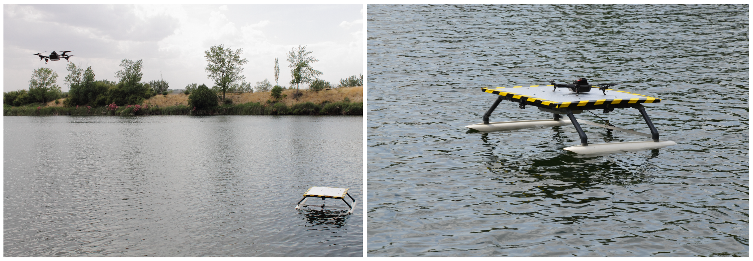
Our aim is that this vehicle supports small USVs remote sensing in fluvial environments, which are easy to replicate, portable, and have an affordable market price (most of the vessels referenced in the literature for which data is available have prices above the thousand euros mark). Figure 1 illustrates a possible scenario where the proposed system can be used.
3. Materials and Methods
This section describes the prototype design and the different tasks that made up its construction. This includes the chassis construction, the sizing of the actuators, both the motor and the servo motor controlling the rudder and the on-board electronics as well as the needed mechanical elements for the operation of the vessel. A detailed list of materials and costs can be found in the project’s repository under the Supplementary Materials Section.
Before starting to develop the USV a set of system requirements have been defined. The vessel must be able to carry its instrumentation and additional electronics along with a big enough payload associated with most common drone models. It must provide an interface for its teleoperation and autonomous control. Portability must be optimized to make access to study sites easy. Low-cost manufacturing is considered to make possible eventual deployment of multiple units for wide area coverage. In addition, finally, the vessel must have enough autonomy to cover survey and/or tracking missions while maintaining a cruise speed suitable for such missions. Table 1 summarizes and lists the aforementioned system requirements.
Concerning the environment and its effect on the design parameters, still calm waters have been considered. This assumption fits the expected operation conditions of the platform in inland waters. Current speed in rivers and fluvial lakes where the vessel will operate are low and often negligible, aided too by the low profile of the hulls. Nevertheless, to take into account the possible inaccuracies of the used approach and the assumptions made, a cruise speed five times higher than required has been used for the design. This leaves room for faster cruise speeds and includes a wide margin of safety to overcome factors not considered during the design.
3.1. Chassis Construction
For the prototype design and construction, several requirements had to be considered. First, a wide platform surface was needed that offers a large margin of error at the time of landing, as well as good compatibility with different UAV models. This way, the device would have a high versatility. The use of PVC as material for the vehicle structure, was chosen for its optimal resistance in relation to volume and weight. For the shape of the base, PVC elbows and Ts were put together with slow drying glue. Through this method, an easy assembly was achieved. Furthermore, remote-controlled hydroplane skates with a high flotation capacity for contact with water were placed as the key element for the platform. A light surface with wide landing area was essential, thus a polyurethane foam, a low-density material that has good resistance, was used. A 90° aluminum plate to carry the rudder was placed in the vessel, connecting the two rear legs of the base, and allowing its movement. Finally, a waterproof electrical box under the landing surface was needed to include the necessary electronics.
3.2. Motor and Rudder Servo Sizing
To select the necessary hardware for the vessel an analysis of the forces acting on the body and rudder of the vessel was performed. This analysis will help define the requirements related to engine power and the rudder servo minimum torque.
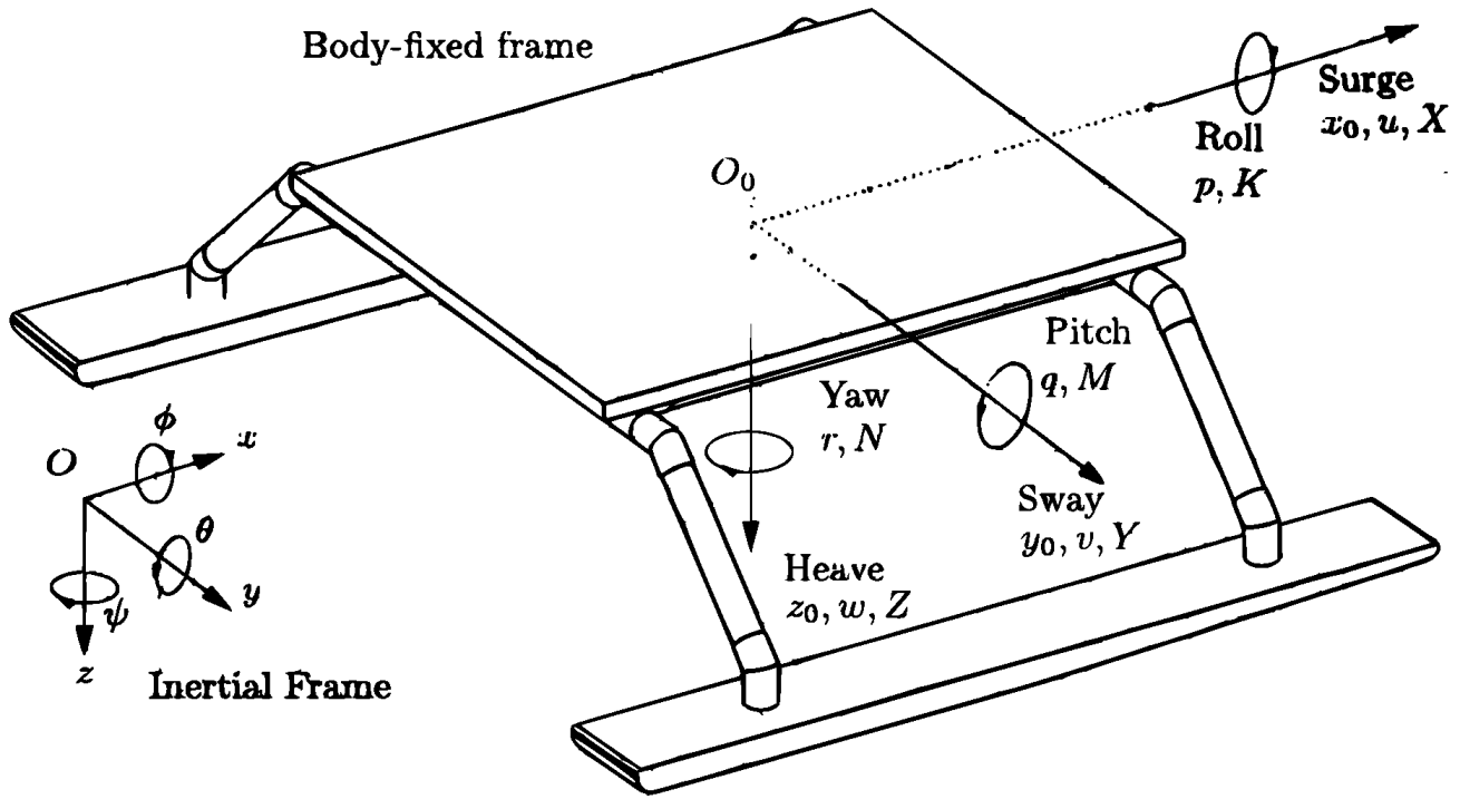
For this analysis we will first set a suitable workspace for notation. The Strider V1.0 was considered as a single rigid solid [20], with an inertial reference frame attached to the Earth and a body-fixed reference frame. The inertial frame was defined with the standard notation of SNAME (Society of Naval Architects and Marine Engineers), following the NED convention, pointing North, East and Down respectively (see Figure 4).
Angular motion is defined in terms of the Euler angles being the roll, pitch and yaw angles respectively as shown in Figure 4. We will also define and as the angular velocities and the torques about the and directions with respect to the body frame.
Concerning linear motion, stands for the linear position of the body-fixed frame with respect to the body-fixed frame. While stands for the linear velocity of the vessel and for the forces and torques applied to the body, both referenced in the body-fixed frame. Motions on the direction are usually called surge, sway, and heave, respectively.
We start the analysis by using Newton’s second law, to describe translational motion:
where is the mass of the vessel. From this expression we can then divide the force vector into its different components to analyze the forces applied to the body of the vessel. This description of the force vector is really simple but sufficient for motor sizing.
where and are air and water drag horizontal forces derived from movement through both fluids and is the thrust produced by the propeller. is the buoyancy force and are other forces not considered under normal operation such as exogenous forces or forces not relevant or considered for motor sizing.
Since the only force opposing the thrust force of the vessel, disregarding for motor sizing, are and we will characterize them to obtain the necessary motor power to move the vessel.
Now, for the calculation of air and water resistance, a fluid dynamics approach was used. Reynolds number was calculated using Equation (3) to characterize drag forces in both fluids.
where and are the density and dynamic viscosity of the studied fluid, u is the surge speed as described by Figure 4 and is the characteristic length of the drag surfaces. Reynolds number characterizes the type of flow (laminar or turbulent) of the fluid, which affects the calculation of the friction coefficient :
With this in mind, we can calculate the drag forces opposing surge motion by identifying all the contact surfaces that contribute to the drag, both in water and air. Figure 5 shows all the surfaces contributing to the drag force and their fluid of origin, which lets us, in conjunction with Equation (6) calculate all the surge drag forces at play.
where is the density of the fluid which drag force is being calculated, u is the surge speed, is the friction coefficient and is the front surface area of the marked elements in Figure 5. A value of surge speed was selected to ensure compliance with the requirements established by Table 1. The high value (regarding the requirement) of this design parameter selection is due to the necessity of a safety margin due to the possible inaccuracies of the model and assumptions made. This also ensures the inclusion of top speed headroom above the required cruise speed.
We can calculate then the necessary power to overcome the surge drag forces as:
where is the sum of all surge drag forces and u is the surge speed.
3.2.1. Motor Sizing
Now that we have established a way to model drag forces we can determine the necessary power for the motor of the Strider V1.0. We can start by remembering the relationship between motor power , torque and angular velocity :
Now, using the above equation and Equation (8), where we take into account that the torque is expressed as the product of a force times a radius of action we obtain the following expression:
where is the real necessary power of the motor, is the motor angular velocity, is the radius of action of the motor, is the sum of all the drag forces in the surge direction. is a performance coefficient bigger than one that corrects the theoretical power to the real necessary power taking into account the efficiency of the motor (taken as the average performance coefficient for electrical motors ), other smaller contributions to the drag forces not taken into account while sizing and absorbs the term.
3.2.2. Rudder Servo Motor Sizing
The vessel is oriented through the rudder action, which movement is executed by a servo motor. Concerning its sizing the forces produced over the surface of the rudder in operation were considered. The force exerted was calculated with the distribution of pressures on its surface:
where is gravitational acceleration, is the rudder length, its width and the vertical that corresponds to the height in a Cartesian coordinate system. Through the rudder action radius, the torque exerted by the servo is expressed by:
For the setup of the Strider V1.0 the values of this design parameters are and .
3.3. Embedded System and On-Board Electronics
The USV was equipped with a central control unit and a perception system. These components were chosen to comply with the minimum cost requirement and enable different navigation modes. The sensors that made up the perception system are detailed bellow and shown in Figure 6:
- HC SR04 ultrasonic sensors for obstacle detection, with a range of 4 m.
- IMU GY-85. Inertial measurement unit with nine degrees of freedom since it features three axis acceleration, gyroscopic and magnetic field measurements. The IMU is used to obtain the acceleration (and speed), the attitude and the heading of the vessel. The speed of the vessel is obtained through integration of the filtered acceleration values obtained by the IMU. It is in a separate box, outside the electronics box to suppress the disturbances that might be caused by the influence of the motor’s magnetic field. Attached to the surface through a sponge to absorb vibrations.
- GPS GY-NEO6MV2, for obtaining the platform position. The GPS module was placed at the top of the platform, and includes: the GPS module, a ceramic antenna, and a voltage divider to enable the Arduino ADC reading.
An outline of how the control unit elements are organized and interconnected is presented in Figure 6. Figure 7 shows the system architecture used for the system. The on-board elements marked in the figure are listed below and labeled in the figure:
- Arduino Mega 2560 processor. The selection of the model was due to the large number of pins required. A basic model such as the Arduino Uno might be insufficient.
- L298N motor controller. Controller for engine power control and direction of rotation.
- HC 06 Bluetooth Board. Enables remote control of the platform through a Smartphone application.
- XBee-xbp24 antennas For wireless connection within a 1 km of range.
- 4000 mAh Battery (7.2 V). For long period power supply for the system.
- MicroSD Reader Catalex is used as a black box, records system navigation data.
- Battery measurement. The platform is equipped with a battery management system. When the battery is low, a buzzer is activated, giving an acoustic signal that alerts the user when the battery needs to be recharged.
- Servo HDKJ D3015 for turning the rudder during vessel operation. It features a maximum torque of 2.5 Kg cm.
- Electric motor thrust, with 43 W of power and a 7.2 V input voltage.
3.4. Mechanical Elements
The set of elements in charge of making the operation of the prototype possible is composed of:
- Torque Reducer 3:1. For the purposes of this project, a greater force is required to move the total weight of the system, which includes the structure and the landed drone. For this purpose, a gearbox was used to increase the torque exerted by the engine while reducing the angular speed. The gear ratio of the used torque reducer is 3:1.
- Propeller. Converts the rotation motion of the shaft into propulsion for the vessel.
- Drive shaft. It transmits the movement from the output of the reducer to the propeller introduced in the water. It is made of stainless steel to prevent deformation and corrosion.
- Cardan. Articular linkage between the gearbox and the transmission shaft. Allows transmission of rotary motion.
- Rudder. Control device used to produce steering forces in the vessel and change the heading.
You can see in Figure 8 the layout of these elements.
4. Modeling and Control
This section provides a dynamic model of the vessel based on Maneuvering Theory which is then used implemented in a simulator. A simple controller and a waypoint-based algorithm is implemented to showcase some of the capabilities of the simulator. The objective of the simulator is to eventually be a platform for prototyping control strategies before their deployment in the real robot, reducing development and debugging time.
Besides the dynamic model and its applications, this section describes the implemented navigation modes whose controllers can be found in the accompanying open-source repository of the USV, it being a teleoperated mode and an autonomous obstacle avoidance controller.
4.1. Dynamic Modeling
The application of model-based design approaches to controller prototyping allows for quick deployment and debugging of control strategies before implementing them in the real platform. For the Strider V1.0 a dynamic model has been obtained and can be used to evaluate more complex control policies that can be implemented in the future.
There exist many different approaches to surface vessel dynamic modeling. In [21] a wide array of different models for the description of the vessel motion are covered.
For the Strider V1.0 model, a Maneuvering Theory approach was used. It considers the vessel’s movement at a constant positive speed or with small variations. Only surge, sway and yaw of the vessel are considered due to its assumption of calm waters and low swell. Besides this, we will make the following assumptions due to the symmetry and small size of platform:
- The body-fixed frame axes coincide with the principal axes of inertia of the body
- The moments of inertia are constant.
- Body symmetry with respect to the center of mass is assumed.
- The body-fixed frame origin is coincident with the center of mass.
- Restricted, calm, and still-water bodies are assumed. This implies that no currents or waves affect the motion of the ship.
- Heave, roll and pitch motions are neglected due to a zero-frequency wave excitation assumption.
- Surge motion is decoupled from sway and yaw motion due to the symmetry of the vessel hulls.
- Added mass effects on the hulls are neglected since only steady motion will be considered.
If we deem the previous points and the symmetry of the boat fixed axes, we obtain the following expression, derived from the general motion equation for a rigid solid considering the made assumptions. A more detailed description of the dynamic model development and the components of the force and torque vectors can be found in [20]:
where is the mass of vessel and is the diagonal inertia matrix with respect to the body frame. If we apply the assumptions under Maneuvering Theory, the obtained expression from the simplified above matrix equation is:
4.1.1. Example Controller and Simulation
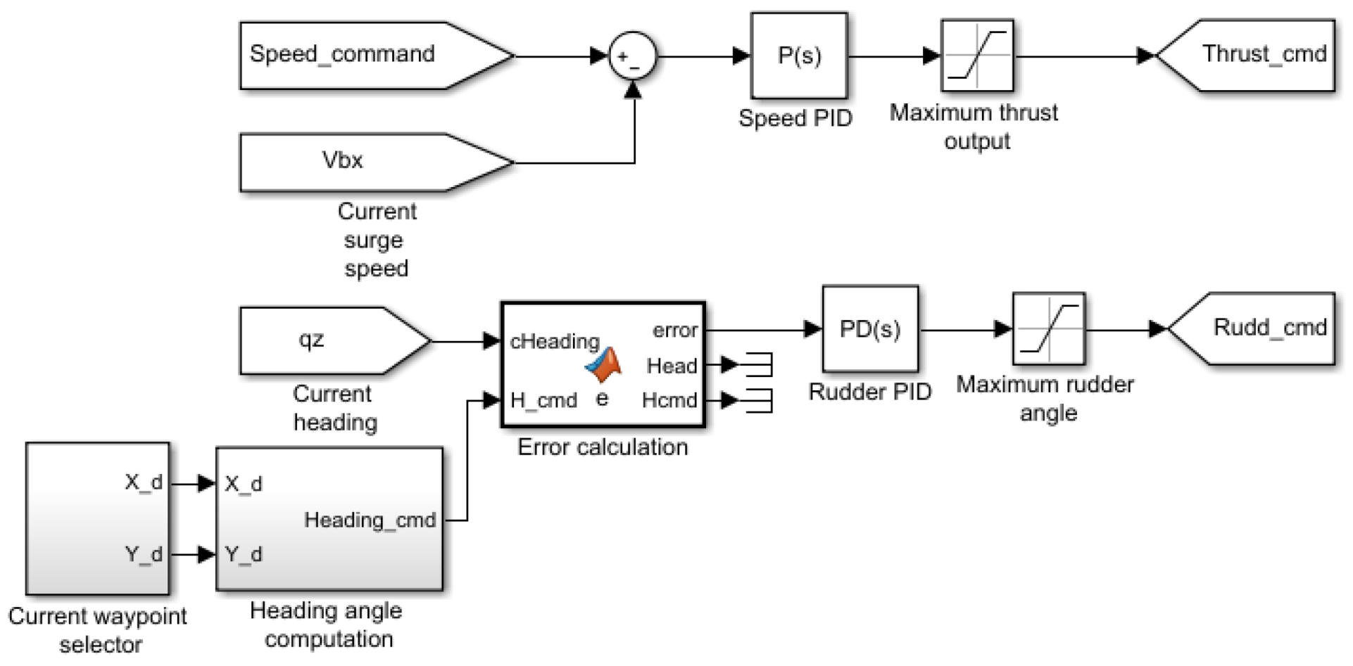
From this model, a suitable controller for the system can be prototyped. As a showcase of the capabilities of this model-based design (MBD) approach and to eventually use the model for quick prototyping, a tracking algorithm based on route points was implemented. Waypoints are represented by latitude and longitude coordinates () for representing an ordered database of points, as seen in Equation (16). Two PID-based (P and PD) controllers were used for orientation and speed (through the rudder and the propeller). The control architecture is depicted in Figure 9.
The desired orientation angle from the position of the vessel ( regarding the inertial frame) was obtained from the expression in Equation (17). The calculation of the desired angle does not take into consideration the landing platform heading. Moreover, the calculation of a final heading when reaching a point was not considered in this work as a line-of-sight guidance approach was used. The expression has been written in latitude and longitude terms, coinciding with the inertial frame shown in Figure 4, following the NED convention.
where and are current the latitude and longitude of the vessel and and de selected waypoint coordinates. Once a waypoint has been reached, the next waypoint () is selected, resulting in a new . For this purpose, the concept of circle of acceptance is adopted. Once the vessel is within a circle of radius m the next waypoint is selected.
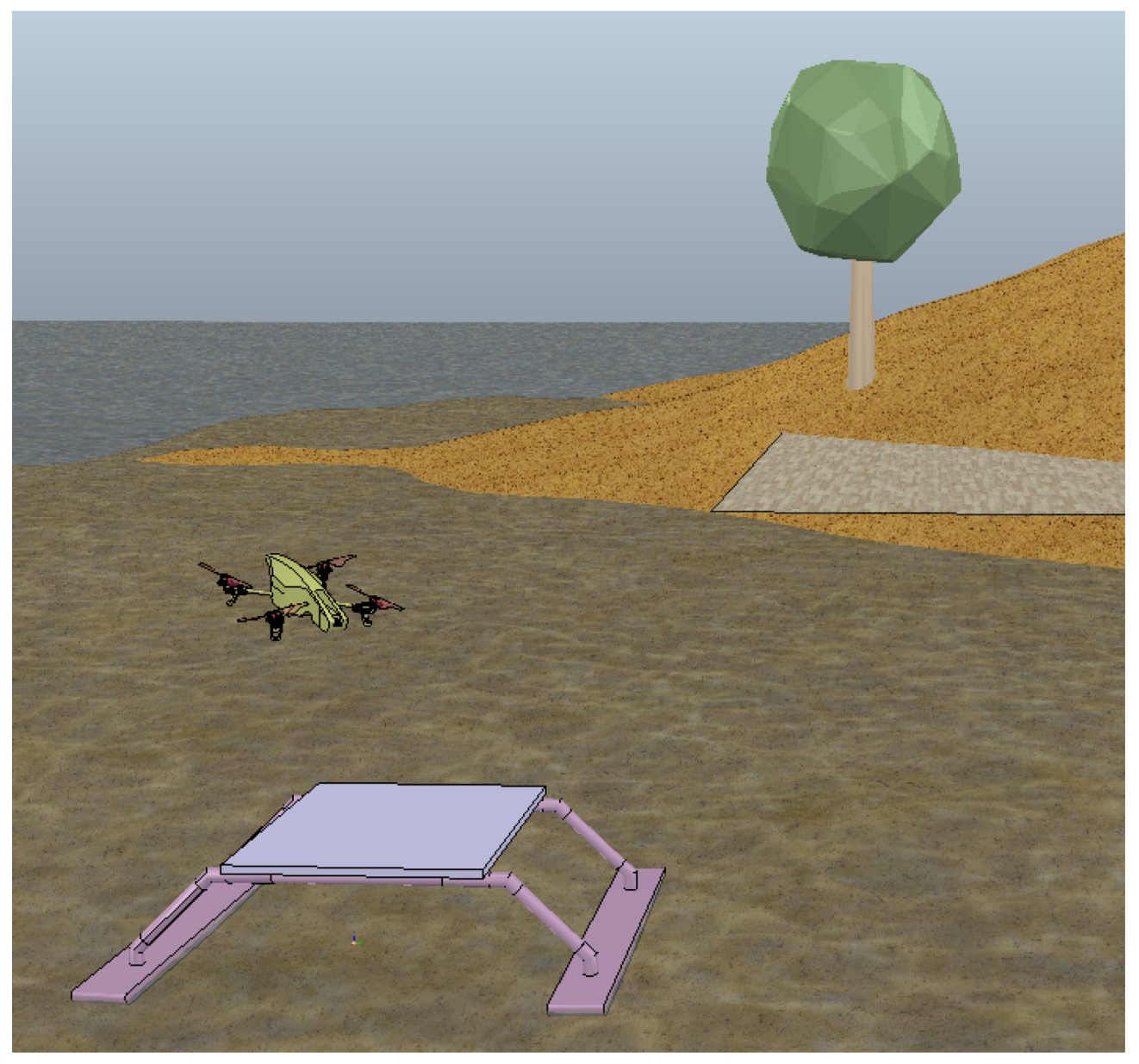
The simulation of the model was implemented using V-REP while the control architecture was built in MATLAB/Simulink. Figure 10 shows a screenshot of the simulation environment (which is also able to simulate UAVs and interaction between both robots).
4.2. Navigation Modes
The prototype has two different navigation modes: Manual, through a teleoperation device (remote control) by the user. In addition, with an algorithm that calculates forthcoming actions, based on the obstacles present in its trajectory, while trying to keep a constant surge speed and heading selected by the user.
4.2.1. Teleoperated
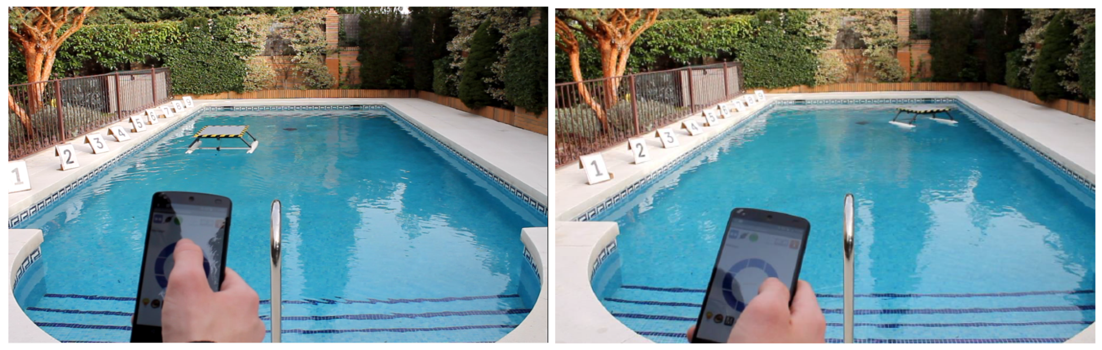
The remote control can be handled by two different methods of communication: Via a smartphone application for Android, programmed for simple commands, using a Bluetooth connection to the control base. In addition, via a PC, with a XBee PC-Prototype connection. Figure 11 shows the tele-operation interface being used during a test. A video showcasing this feature can be found in the Supplementary Materials Section.
Both methods have an eight directions discrete joystick control and it is possible to adjust the speed for each situation, with a toggle option for manual and automatic control modes. On the smartphone mode, the platform parameters and the sensors readings are recorded in a micro SD card, while on the PC option it is also possible to visualize the information in real time.
4.2.2. Obstacle Avoidance
The programming of the autonomous obstacle avoidance controller was carried out following the fundamental idea of reactive behavior. This is described as an action-reaction system. An immediate response to a stimulus received from its environment [23]. This obstacle evasion function responds to the necessity of maneuvering in complicated environments. For this, the proportional control law detailed below has been used:
is a controller command parameter to send to the servos, k is the regulator gain determined by the Ziegler-Nichols method, and the is the difference between the distance set as safe and the obstacle to evade (Safe distance has been taken as 0.5 m). In relation to this, if we define the distance that the sensor measured towards the obstacle as , and the safety distance of the platform as , we can describe two possible scenarios with lateral obstacles in the following way:
1. . When the distance to the obstacle measured by the sensor is greater than twice the safety limit, there is no reaction from the system.
2. . Between the safety distance and its double, the response is proportional, namely, as the obstacle to evade approaches, the rudder updates its position in real time proportionally until the maximum rotation angle is reached. In this way, there is a constant regulation of the rotation angle of the platform with an optimal response for each situation.
In case of a frontal obstacle, the system will retreat, turn, and move away until a safe distance is reached to resume its new direction.
5. Results
This section collects the results of the performed tests and experiments. Tests performed with the real vessel were performed to ensure the correct functioning and design specifications. The performed tests correspond to the three navigation modes from Section 4.2. They are accompanied by test results from the simulation environment, using the obtained dynamic model of the vessel, showing similar dynamics, and showcasing its quick prototyping possibilities. Simulation tests show three setups with the controllers from Section 4.1.1.
Test environmental conditions during the real and simulated tests were similar. Wind speed and water current were minor and negligible at the time of testing. For the simulation, only sensor noise was added to the speed and heading controllers to equate test conditions. These conditions are close to the expected operating conditions of the multi-robot system, as it is intended for calm inland water environments where water flow and wind speeds are low, conditions needed for correct operation and data collection with the UAV robot.
5.1. Manual and Autonomous Mode
Three different tests with the real platform were carried out: two in manual mode using a smartphone to send commands, and one in autonomous mode. The aim of these tasks are to show the correct performance of the platform, including the control of the structure by the requirements of the user and the algorithm calculations avoiding obstacles. The heading and speed commands presented in the figures of this section represent the reference values given to the operator of the vessel to track them during the experiments.
5.1.1. Manual Mode: Straight Line
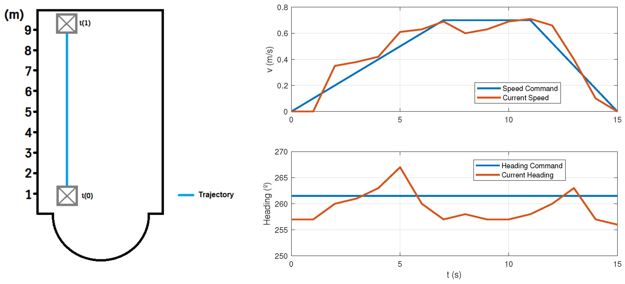
A straight-line trajectory was performed to observe the efficacy of the vessel’s propulsion system and course keeping. Figure 12 shows the results obtained during the test. Three speed profiles where commanded: first an acceleration command, an intermediate section with constant speed, and a final breaking phase. In the intermediate part, slight variations of speed by corrections on the trajectory can be seen.
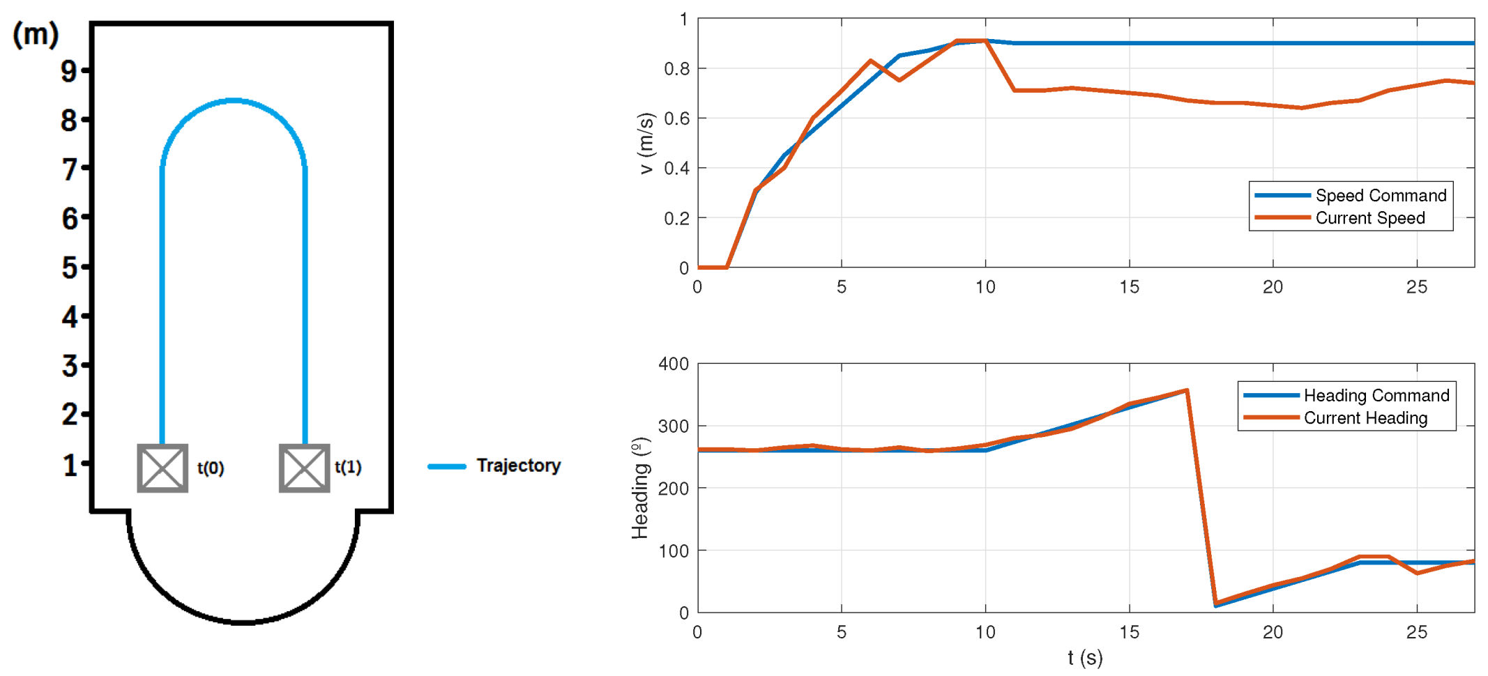
5.1.2. Manual Mode: U
This test is similar to the previous one, but presents a mid-travel change in the orientation (t = 8 s), performing a U-shaped trajectory. Figure 13 shows the speed and heading profiles during the test. As it can be seen from the plots, reference tracking for heading is good. Reference tracking for surge speed shows an offset once the turning maneuver starts, due to the offset between the velocity of the vessel and the surge speed when the yaw angle changes (sway speed appears). This offset remains constant and once the turning maneuver finishes speed values stabilize around the commanded speed.
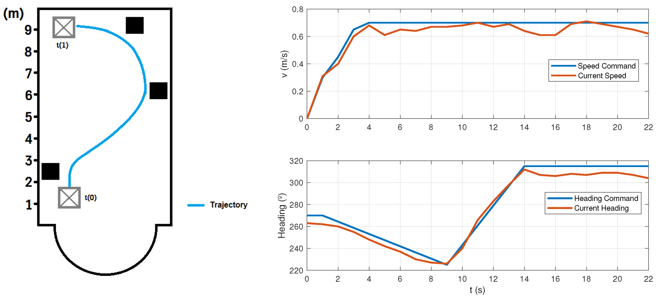
5.1.3. Autonomous Mode with Obstacle Evasion
In this mode, the USV can maintain a determined surge speed (controlled by manual feedback) while autonomously avoiding potential obstacles using the algorithm described in Section 4.2.2 by changing its heading. This allows to perform safe roaming maneuvers finding and obstacle free path. In this experiment a set of obstacles have been placed to demonstrate the behavior of the logic implemented. In this experiment the controller parameters were set at and for the proportional gain and offset parameter, which yielded the best results.
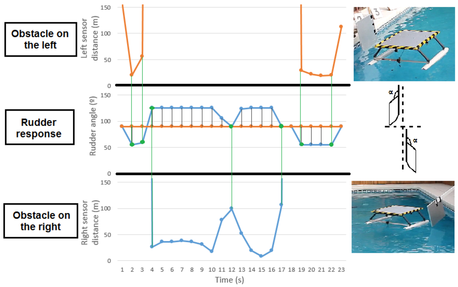
We can observe in Figure 14a significant change of orientation of the platform at times t = 4 s, t = 12 s and t = 19 s, moments where the obstacles were detected. Again, we see the small dip in speed due to the change in orientation; however, for these small heading changes, the offset regarding the reference and the rising time to the commanded speed is much faster and barely noticeable. Figure 15 shows the measurements read by the right and left sensors, and the rudder response during the test (where the neutral position of the rudder is 90°).
5.2. Simulation Results
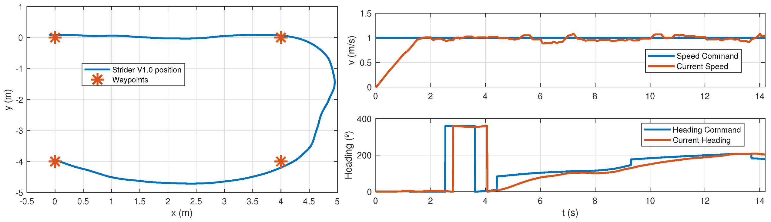
Concerning the performed simulations, we will showcase three test runs. The tests will use the implemented waypoint tracking algorithm and P and PD-based controllers for the surge speed and heading of the vessel respectively from Section 4.1.1. The three simulated runs correspond to a U-shaped and a straight-line trajectory and a GPS waypoint trajectory tracking. The presence of heavy disturbances was neglected because this vehicle was not developed to navigate in the sea, but in calm inland water environments where the oscillations are approximately null. Nevertheless, an effort was made to introduce noise in the regulators.
The implemented controllers for surge speed and heading where tuned using an initial estimate from a Ziegler-Nichols’ tuning and then fine-tuned manually to a rise time below 2 s and no oscillations. The final gains for both controllers where for the surge speed controller and for the heading controller, where are the proportional and derivative gains and the filter coefficient respectively. The radius of acceptance used was m.
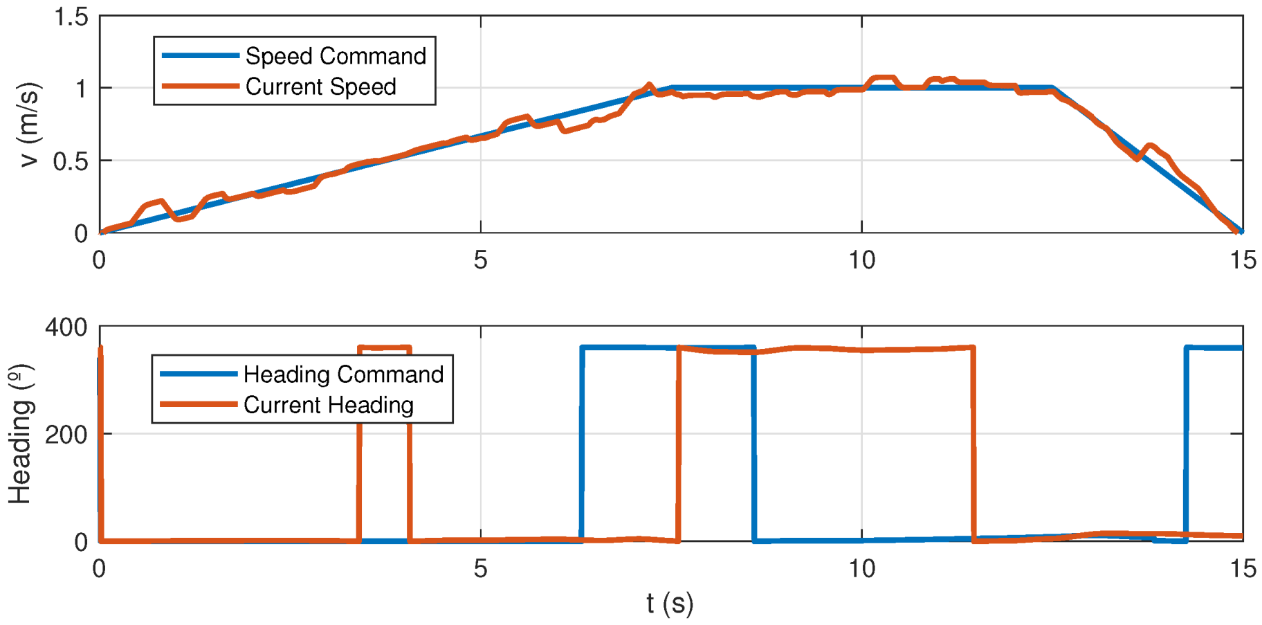
Figure 16 shows the results for a “U” shaped trajectory simulation with added noise (Gaussian) at the controller input, to evaluate their performance. Figure 17 also illustrates velocity and heading tracking in a straight-line trajectory under noise. The heading angle convention used measures clockwise from north in degrees 0° to 359°, where 0° is north, 90° east, 180° south and 270° west. Sensor noise has been modeled as white noise with zero mean and and standard deviation. Sample time for the noise was . As it can be seen from the results, the implemented controllers are sufficiently robust to deal with the noise while maintaining control of the vessel.
6. Discussion and Conclusions
With the aim of flying a UAV over fluvial environments, a mobile platform was designed and developed as a support vehicle. Among the main features of this platform are its low cost of manufacturing (less than 500 euros), ease of transport (weight less than 5 Kg and its dimensions are less than 1 m) and ease of control using a mobile phone or PC.
The built platform can carry different UAV models and meets all the design requirements indicated in Table 1. This was possible due to the combination of lightweight and affordable materials such as PVC, polyurethane, and electronics such as Arduino. The simplicity of the design implies easy maintenance and repair of the vessel, without disregarding any of the design requirements, and contributes to its low price. Table 3 lists the fulfilled design requirements set along a short description. For more detailed and additional information on the requirement fulfillment please refer to the project’s repository included in the Supplementary Materials Section.
Furthermore, a dynamic model from the built platform was also obtained to provide a rapid channel for control prototyping and system configuration without the need to carry out test directly in the physical platform.
To evaluate the success of the design several experiments were performed with the vessel. Real tests demonstrate the capabilities and robustness of the platform and showcase the use of the implemented navigation modes from Section 4.2. Simulation tests verify the suitability of the vessel model and the performance of the P and PD controllers for speed and heading, respectively. Noise disturbance rejection of the implemented controllers in simulation tests yielded stable behavior under disturbances and exogenous effects. Considering the simplicity of the control architecture, the achieved results are sufficient for the given application, although better control schemes can be designed and applied in the future.
Using the obtained dynamic model for prototyping and deploying controllers has proved to be a good approach to reduce deployment and development time while testing in a risk-free environment. As future work, it is intended to develop a second prototype with more sensory and processing capacity to test further control schemes and collaborative behaviors with the UAVs in different environment conditions. For example, the speed of the vessel is achieved via integration of the acceleration values obtained from the IMU. Although this method suffers from some drift in the values in long tests an EKF fusing GPS and IMU data to obtain velocity will be implemented in the future. Further modifications will also be done in the landing base to enable the attachment of backpack strips for easier transportation by a person.
Finally, to the best of our knowledge this is the smaller double-hull USV ever built and we believe that will be an added value point in future aerial remote sensing mission in aquatic environments.
Supplementary Materials
The source code of the prototype and the video with the tests performed can be acquired in the following links respectively: github.com/davodav93/Strider and youtu.be/8sj1Q5ENeWA.
Author Contributions
Design, D.B. and J.V.; Manufacturing, D.B.; Trials and validations, D.B. and O.V.; Modeling and control, O.V.; Writing—review and editing, D.B., J.V. and O.V.
Funding
The research leading to these results has received funding from the RoboCity2030-III-CM project (Robótica aplicada a la mejora de la calidad de vida de los ciudadanos. fase III; S2013/MIT-2748), funded by Programas de Actividades I+D in Comunidad de Madrid and cofunded by Structural Funds of the EU.
Conflicts of Interest
The authors declare no conflict of interest.
Abbreviations
The following abbreviations are used in this manuscript:
| COLREGs | International Regulations for Preventing Collisions at Sea 1972 |
| EU | European Union |
| EKF | Extended Kalman Filter |
| IMO | International Maritime Organization |
| NED | North, East, Down |
| PID | Proportional Integral Derivative |
| PVC | PolyVinyl Chloride |
| SNAME | Society of Naval Architects and Marine Engineers |
| UAV | Unmanned Aerial Vehicle |
| USV | Unmanned Surface Vehicle |
References
- European comission. A Healthy and Sustainable Environment for Present and Future Generations; The European Union Explained; Unión Europea: Bruselas, Belgium, 2014. [Google Scholar]
- Oscoz, J.; Martínez, J.G.; Ector, L.; Sánchez, J.C.; Pardos, M.; Durán, C. A comparative study of the ecological state of the Ebro watershed rivers by means of macroinvertebrates and diatoms. Limnetica 2007, 26, 143–158. [Google Scholar]
- Peãa, R.; Serrano, M.L.; Ruiz-verdú, A. Studies of impact on fluvial ecosystems by airborne remote sensing: Thermal discharges in river Tajo and suspended solids diffusion in rivers Esera and Cinca (Spain). Limnetica 1999, 16, 99–107. [Google Scholar]
- Díaz-Paniagua, C.; Aragonés, D. Permanent and temporary ponds in Doñana National Park (SW Spain) are threatened by desiccation. Limnetica 2015, 34, 407–424. [Google Scholar]
- Zhang, C.; Kovacs, J.M. The application of small unmanned aerial systems for precision agriculture: A review. Precis. Agric. 2012, 13, 693–712. [Google Scholar] [CrossRef]
- Cândido, A.K.A.A.; Filho, A.C.P.; Haupenthal, M.R.; da Silva, N.M.; de Sousa Correa, J.; Ribeiro, M.L. Water quality and chlorophyll measurement through vegetation indices generated from orbital and suborbital images. Water Air Soil Pollut. 2016, 227, 224. [Google Scholar] [CrossRef]
- Morsy, S.; Shaker, A.; El-Rabbany, A. Using multispectral airborne LIDAR data for land/water discrimination: A case study at Lake Ontario, Canada. Appl. Sci. 2018, 8, 349. [Google Scholar] [CrossRef]
- Dunbabin, M.; Marques, L. Robots for Environmental Monitoring: Significant Advancements and Applications. IEEE Robot. Autom. Mag. 2012, 19, 24–39. [Google Scholar] [CrossRef]
- Rodríguez, J.M.R.; Hernández, J.J.D.; de Betoño, C.M.F. Estándares de interoperabilidad europea en los sistemas marítimos no tripulados. In Proceedings of the 53 Congreso de Ingeniería Naval e Industria Marítima, Cartagena, Spain, 9 October 2014. [Google Scholar]
- Wang, T.; Wu, C.; Wang, J.; Ge, T. Modeling and control of negative-buoyancy tri-tilt-rotor autonomous underwater vehicles based on immersion and invariance methodology. Appl. Sci. 2018, 8, 1150. [Google Scholar] [CrossRef]
- Sun, X.; Wang, G.; Fan, Y.; Mu, D.; Qiu, B. An automatic navigation system for unmanned surface vehicles in realistic sea environments. Appl. Sci. 2018, 8, 193. [Google Scholar] [CrossRef]
- Arrichiello, F.; Das, J.; Heidarsson, H.; Chiaverini, S.; Sukhatme, G.S. Experiments in autonomous navigation with an under-actuated surface vessel via the Null-Space-based Behavioral control. In Proceedings of the 2009 IEEE/ASME International Conference on Advanced Intelligent Mechatronics, Singapore, 14–17 July 2009; pp. 362–367. [Google Scholar]
- Han, J.; Park, J.; Kim, T.; Kim, J. Precision navigation and mapping under bridges with an unmanned surface vehicle. Auton. Robot. 2015, 38, 349–362. [Google Scholar] [CrossRef]
- Seedhouse, E. SpaceX’s Dragon: America’s Next Generation Spacecraft, 1st ed.; Springer International Publishing: Basel, Switzerland, 2016. [Google Scholar]
- Von Ellenrieder, K. Free running tests of a waterjet propelled unmanned surface vehicle. J. Mar. Eng. Technol. 2013, 12, 3–11. [Google Scholar] [CrossRef]
- Caccia, M.; Bruzzone, G.; Bono, R. A Practical Approach to Modeling and Identification of Small Autonomous Surface Craft. IEEE J. Ocean. Eng. 2008, 33, 133–145. [Google Scholar] [CrossRef]
- Bertaska, I.R.; Shah, B.; von Ellenrieder, K.; Švec, P.; Klinger, W.; Sinisterra, A.J.; Dhanak, M.; Gupta, S.K. Experimental evaluation of automatically generated behaviors for {USV} operations. Ocean Eng. 2015, 106, 496–514. [Google Scholar] [CrossRef]
- Djapic, V.; Prijic, C.; Bogartz, F. Autonomous takeoff landing of small UAS from the USV. In Proceedings of the OCEANS 2015—MTS/IEEE, Washington, DC, USA, 19–22 October 2015; pp. 1–8. [Google Scholar]
- Pinto, E.; Marques, F.; Mendonça, R.; Lourenço, A.; Santana, P.; Barata, J. An autonomous surface-aerial marsupial robotic team for riverine environmental monitoring: Benefiting from coordinated aerial, underwater, and surface level perception. In Proceedings of the 2014 IEEE International Conference on Robotics and Biomimetics (ROBIO), Bali, Indonesia, 5–10 December 2014; pp. 443–450. [Google Scholar]
- Velasco, O.; Blanco, P.J.A.; Valente, J. Smooth autonomous take-off and landing maneuvers over a double-hulled watercraft. In Proceedings of the 14th International Conference on Informatics in Control, Automation and Robotics ICINCO, INSTICC, Madrid, Spain, 26–28 July 2017; SciTe Press: Setubal, Portugal, 2017; Volume 2, pp. 389–396. [Google Scholar] [CrossRef]
- Fossen, T.I. Handbook of Marine Craft Hydrodynamics and Motion Control; John Wiley & Sons: Hoboken, NJ, USA, 2011. [Google Scholar]
- Ardumotive Arduino Greek Playground. 2018. Available online: http://www.ardumotive.com/ (accessed on 5 July 2018).
- Murphy, R.R. Introduction to AI Robotics; MIT Press: Cambridge, MA, USA, 2000. [Google Scholar]
Figure 1.
The above figures illustrate a possible collaborative mission between an aerial robotic system and the Strider V1.0 in a fluvial environment.
Figure 1.
The above figures illustrate a possible collaborative mission between an aerial robotic system and the Strider V1.0 in a fluvial environment.

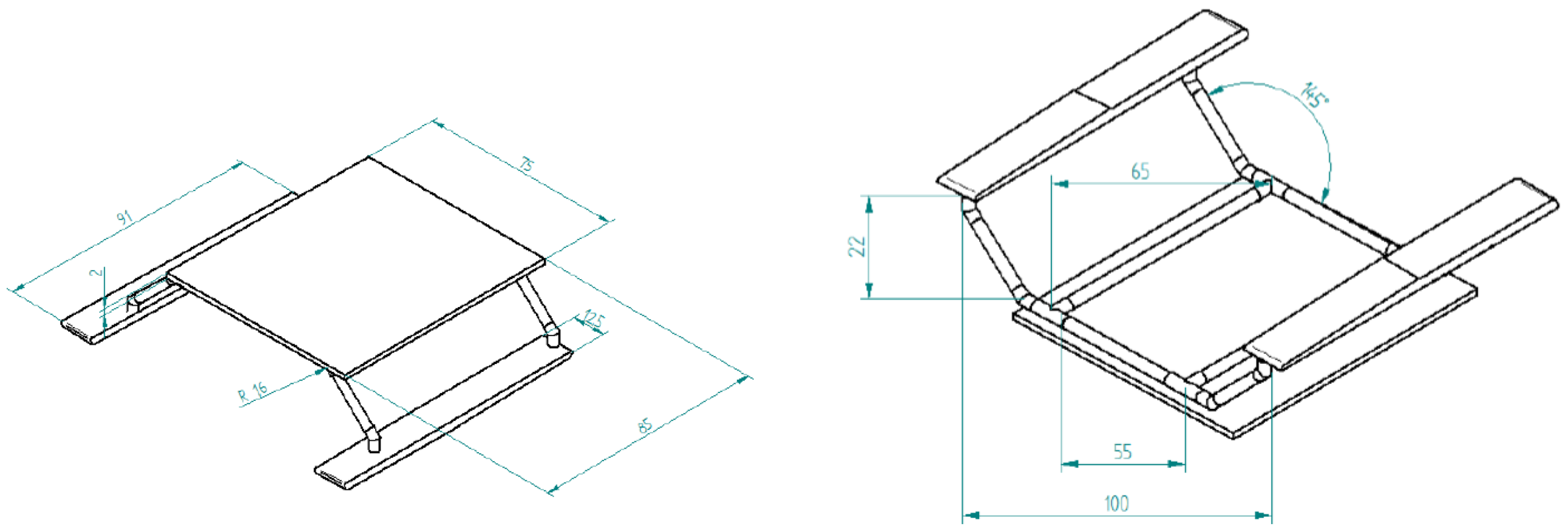
Figure 2.
Top and bottom view of the CAD design.

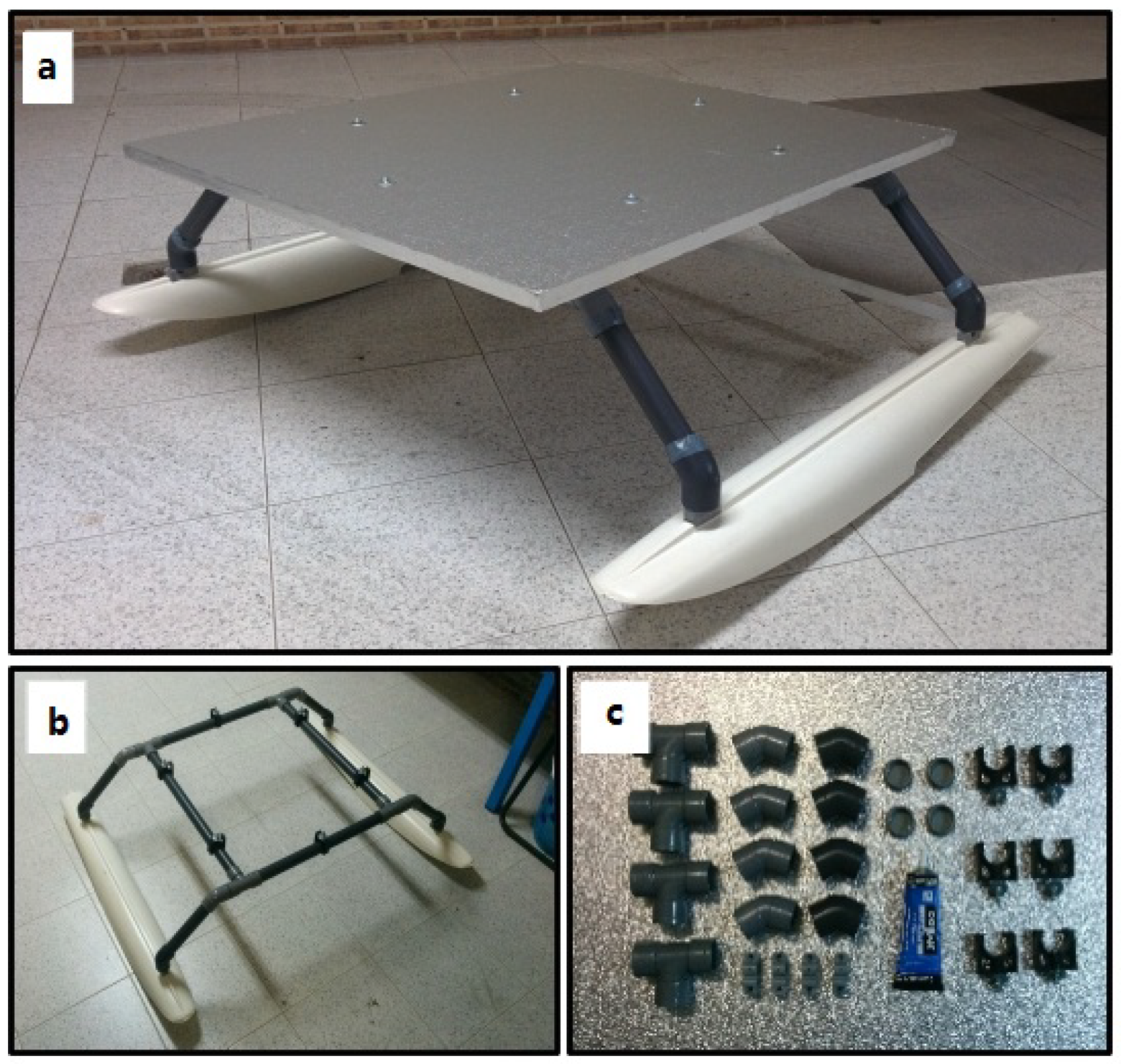
Figure 3.
Material used in the structure construction: (a) Final assembly, (b) Structure without the polyurethane foam base, (c) The PVC materials used.
Figure 3.
Material used in the structure construction: (a) Final assembly, (b) Structure without the polyurethane foam base, (c) The PVC materials used.

Figure 4.
Standard notation and sign conventions for ship motion description on the Strider V1.0.

Figure 5.
Forces affecting the system. On the left: areas of the skate and landing surface where the water and air resistance forces affect, respectively. On the right: frontal areas affected by air.
Figure 5.
Forces affecting the system. On the left: areas of the skate and landing surface where the water and air resistance forces affect, respectively. On the right: frontal areas affected by air.

Figure 6.
On-board electronics and embedded system. The watertight box with the central control unit was placed in the under the landing pad. The enumerated elements in the figure list the on-board elements present in the system. The GPS was placed in the top of the platform, while the compass was placed underneath.

Figure 7.
General system architecture. Describing the power and communication relationships among the different modules that comprise it.
Figure 7.
General system architecture. Describing the power and communication relationships among the different modules that comprise it.

Figure 8.
Main mechanical elements for propulsion and direction: (a) 3-blade propeller; (b) Rudder; (c) steel transmission shaft; (d) and waterproof servo for rudder control.
Figure 8.
Main mechanical elements for propulsion and direction: (a) 3-blade propeller; (b) Rudder; (c) steel transmission shaft; (d) and waterproof servo for rudder control.

Figure 9.
StriderV1.0 controllers block diagram in MATLAB.

Figure 10.
V-REP simulation environment for testing control strategies and interaction between robots.
Figure 10.
V-REP simulation environment for testing control strategies and interaction between robots.

Figure 11.
Counter-clockwise U turn via remote control using a modified version of the Ardumotive Bluetooth Controller [22].
Figure 11.
Counter-clockwise U turn via remote control using a modified version of the Ardumotive Bluetooth Controller [22].

Figure 12.
Straight-line test results. Position of the Strider V1.0 (Left) and current and reference speed and heading values during test (Right).
Figure 12.
Straight-line test results. Position of the Strider V1.0 (Left) and current and reference speed and heading values during test (Right).

Figure 13.
U-shaped trajectory test results. Position of the Strider V1.0 (Left) and current and reference speed and heading values during test (Right).
Figure 13.
U-shaped trajectory test results. Position of the Strider V1.0 (Left) and current and reference speed and heading values during test (Right).

Figure 14.
Autonomous test results. Position of the Strider V1.0 (Left) and current and reference speed and heading values during test (Right).
Figure 14.
Autonomous test results. Position of the Strider V1.0 (Left) and current and reference speed and heading values during test (Right).

Figure 15.
The upper plot shows the measured distance read by the left side sensor while the lower plot the measurements of the right-side sensor. In the central plot, the rudder response was represented as the rudder angle vs. time. Variations in the rudder angle are produced by the vessel’s response to obstacles.

Figure 16.
Position of the Strider V1.0 during the U-shaped trajectory test (left) and current and commanded speed and heading for the U-shaped trajectory test (Right).
Figure 16.
Position of the Strider V1.0 during the U-shaped trajectory test (left) and current and commanded speed and heading for the U-shaped trajectory test (Right).

Figure 17.
Current and commanded speed and heading for the straight-line trajectory test.

Figure 18.
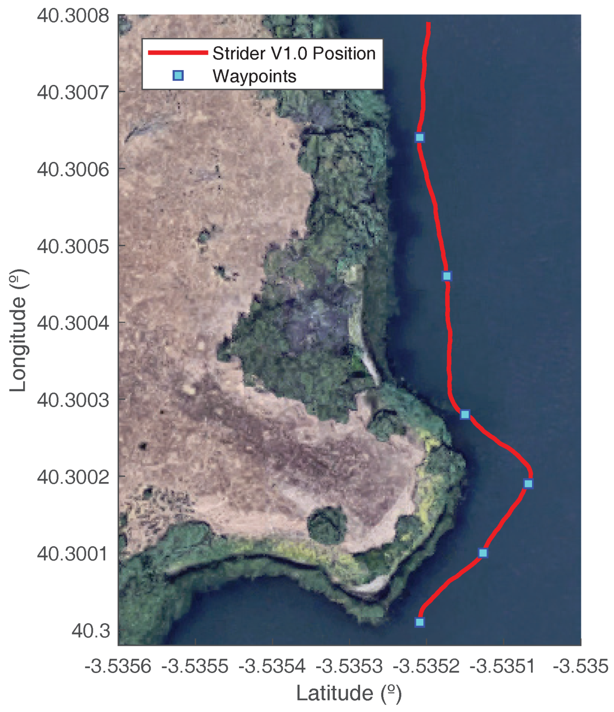
The figure illustrates the trajectory followed by the vessel during the waypoint tracking test. The starting waypoint is the southernmost. The map and coordinates correspond to a testing area for the Strider V1.0.
Figure 18.
The figure illustrates the trajectory followed by the vessel during the waypoint tracking test. The starting waypoint is the southernmost. The map and coordinates correspond to a testing area for the Strider V1.0.


Table 1.
System design requirements.
| Requirement | Description |
|---|---|
| Payload | Ability to carry all the instrumentation and electronics necessary for navigation, as well as an UAV with an area less than 100 cm and a maximum weight of 2.5 Kg. |
| Portability | It can be transported by a person. |
| Speed | Ability to maintain a cruise speed up to 1 m/s. |
| Autonomy | With a range between 30 to 60 min. |
| Teleoperated | Remote control through a Smartphone connection. |
| Automatic | Autonomous navigation and obstacle avoidance. |
| Price | Low-cost manufacturing. |
Table 2.
Ordered waypoint vector with latitude and longitude coordinates.
| Waypoint No. | 1 | 2 | 3 | 4 | 5 | 6 |
|---|---|---|---|---|---|---|
| Latitude (°) | −3.5352 | −3.5351 | −3.5350 | −3.5352 | −3.5352 | −3.5352 |
| Longitude (°) | 40.3000 | 40.3001 | 40.3002 | 40.3003 | 40.3005 | 40.3006 |
Table 3.
System design requirements fulfillment.
| Requirement | Fulfilled | Details |
|---|---|---|
| Payload | Yes | The prototype can carry the chosen UAV with a total payload of 2.5 Kg during the tests while meeting all other design requirements. Please refer to Figure 1 where the Ar. Drone (~2 Kg payload) sits on it. Please refer to the supplementary materials for more detailed information. |
| Portability | Yes | Thanks to the low weight (5 Kg) of the vessel handling of the vessel and transportation is simple. If necessary, it can be easily strapped to the back for ease of transportation to study sites without being excessively cumbersome. Please refer to table provided in the supplementary materials with detailed weights. |
| Speed | Yes | Constant cruise speed of 1 m/s can be achieved by the vessel. Please refer to Figure 13. |
| Autonomy | Yes | Autonomy of the vessel during continuous use was around 60 min. Since the system does not operate at full thrust continuously the 4000 mAh battery achieved almost 60 min of operation during the tests. |
| Teleoperated | Yes | Tele-operation of the vessel is possible and allows remote control of the vessel, either through manual commands or autonomously. Please refer to the video provided in the supplementary materials. |
| Price | Yes | Final price of the vessel was less than 500 €, making this USV platform affordable and accessible. Please refer to table provided in the supplementary materials with detailed costs. |
© 2018 by the authors. Licensee MDPI, Basel, Switzerland. This article is an open access article distributed under the terms and conditions of the Creative Commons Attribution (CC BY) license (http://creativecommons.org/licenses/by/4.0/).
Share and Cite
MDPI and ACS Style
Borreguero, D.; Velasco, O.; Valente, J. Experimental Design of a Mobile Landing Platform to Assist Aerial Surveys in Fluvial Environments. Appl. Sci. 2019, 9, 38. https://0-doi-org.brum.beds.ac.uk/10.3390/app9010038
AMA Style
Borreguero D, Velasco O, Valente J. Experimental Design of a Mobile Landing Platform to Assist Aerial Surveys in Fluvial Environments. Applied Sciences. 2019; 9(1):38. https://0-doi-org.brum.beds.ac.uk/10.3390/app9010038
Chicago/Turabian StyleBorreguero, David, Omar Velasco, and João Valente. 2019. "Experimental Design of a Mobile Landing Platform to Assist Aerial Surveys in Fluvial Environments" Applied Sciences 9, no. 1: 38. https://0-doi-org.brum.beds.ac.uk/10.3390/app9010038
Note that from the first issue of 2016, this journal uses article numbers instead of page numbers. See further details here.