Article

Dynamic Measurement Error Modeling and Analysis in a Photoelectric Scanning Measurement Network

1
State Key Laboratory of Precision Measuring Technology and Instruments, Tianjin University, Tianjin 300072, China
2
Beijing Institute of Spacecraft Environment Engineering, Beijing 100094, China
*
Author to whom correspondence should be addressed.
Submission received: 30 October 2018 / Revised: 13 December 2018 / Accepted: 19 December 2018 / Published: 25 December 2018
(This article belongs to the Special Issue Precision Dimensional Measurements)

Abstract

:

Featured Application

A photoelectric scanning measurement network has the potential for three-dimensional (3-D) dynamic coordinate measurement in industrial manufacturing. It can be applied in aircraft assembly and leveling, digital shipbuilding, tooling monitoring, AGV navigation, and so on.

Abstract

A photoelectric scanning measurement network is a kind of distributed measurement system based on the principle of angle intersection, in which transmitters and photoelectric receivers are the main parts. The scanning lasers in transmitters emit signals and they are obtained by receivers at the measured points. Then the coordinate of the receiver can be calculated by the optimization algorithm. Its outstanding static measurement performance and network scalability capacity give it great potential in large-scale metrology. However, when it comes to moving targets, the angle intersection failure will produce a dynamic error, which limits its further application. Nowadays the research on error modeling and compensation is also insufficient though it has been the crucial concern. In this paper, we analyzed error causes and constructed a dynamic error model. Dynamic error characteristics and the law of propagation were discussed. The measurement uncertainty at different movement speeds was quantized through simulation experiments. To verify the error model, experiments were designed and the dynamic error was evaluated in practice. It matched well with simulations. The model was tested to be reasonable, and provided theoretical support for error compensation.

Graphical Abstract

1. Introduction

The concept of “Industry 4.0” introduces the future trends in industrial development, and the growing interest in intelligent manufacturing has highlighted the need to research novel methods in large-scale metrology [1,2]. Integration of advanced measurement instruments with traditional technologies is recognized as an effective approach to achieve the prospection. Dimensional metrology in manufacturing, which is an important factor for quality insurance, has the characteristics of large measurement range, requirements for high precision and efficiency, and strong environmental interference. In recent years, the breakthroughs in optical technologies and low-cost, fast computers stimulated the wide use of laser tracker and photogrammetry systems. They both provide abundant solutions for three-dimension coordinate measurement [3,4,5].
A laser tracker is based on length measurement by interferometer and angle measurement by encoder. Leica AT series and Faro Vantage series are representatives in this field of research. With sophisticated environmental parameter compensation, they can gain an accuracy of 15 um + 6 um/m and a measurement frequency of up to 1000 Hz. The measurement range is about 80 m. In most cases, it is seen as the benchmark in metrology and gives compensation to positioning error in other instruments [6,7]. However, the laser tracker has its limitations. Firstly, it only conducts single target measurement each time and the efficiency is relatively lower. For example, in large aircraft leveling, hundreds of points on the whole fuselage need to be measured, which may take one or more days. It is time-consuming and unacceptable. Secondly, in a large-scale space, a multi-station network is often necessary for full coverage of the measurement zone. The measurement error is prone to accumulate during coordinate system transformation and distance increase. The system performance will be affected to a great degree [8,9].
Close-range photogrammetry experienced a revolution at the beginning of the 2000s [10] and it has been widely used in applications ranging from automobile manufacturing to aerospace [11,12,13,14,15]. Monocular vision and binocular vision are common solutions for positioning and orientation in large-scale metrology and they enjoy an accuracy of submillimeter. Nevertheless, limited by the image processing and matching algorithm, photogrammetry methods have a relatively lower measurement frequency, which leads to unideal dynamic measurement capacity. Even worse, photogrammetry systems have strict requirements for the environment and measured objects. Light flection from the surface of objects, such as aircraft skin and body-in-white, may lead to low image quality and match failure [16].
In the past few years, we have also witnessed the rapid development of stationary distributed measurement network and it is now widely used in aircraft manufacturing, digital shipbuilding, and tooling monitoring. The workshop measurement positioning system (wMPS) is a representative composed of transmitters, photoelectric receivers, signal processors, and a terminal computer. Each transmitter contains a rotation head and a static base, as shown in Figure 1.
Two line-laser modules are embedded in the rotation head with an intersection angle of 90°. The head rotates about the z-axis of the local coordinate system at a speed of 1500–3000 rev/min. In the static base synchronization lasers are in circular distribution and they will shine when the rotation head goes across the pre-defined reference point in the encoder. The receiver at the measured point obtains the synchronization signal and record it as the start time. After that, laser module 1 and 2 will scan over the receiver in turn. The time difference between synchronization signal and scanning signals is captured through precise timing. It is in a linear relationship with two scanning angles. In this way, the spatial relationship between the transmitter and receiver can be determined solely. Combing signals from multiple transmitters, the coordinate of the receiver can be obtained by the optimization algorithm [17]. At present, the research on static measurement performance of wMPS has been carried out and it gains an accuracy of 0.2 mm + 0.01 mm/m at a frequency of 20 Hz.
However, with the development of industrial automation, dynamic positioning has been increasingly required. In aircraft and ship assembly, large components are carried by industrial robots for docking. The real-time positions of components are necessary for feedback control. Besides, the relative position between different robots is also important to avoid the deformation caused by measurement asynchronization [18,19]. For indoor autonomous guided vehicle (AGV), accurate positioning in global positioning system (GPS) denied conditions is the foundation for navigation and control. On the one hand, wMPS has the potential for dynamic measurement, fast dynamic response, and good static stability. On the other hand, limited by the principle of angle intersection measurement, the error is inherent and non-negligible when the receiver is in motion. Dynamic error analysis and compensation has been the key to further improve the system performance and extend the application area.
In this article, we first introduce the dynamic error causes of wMPS. Then we construct the error model, discuss the error characteristics, and quantize the measurement uncertainty at different cases through simulation experiments. Finally, practical experiments are carried out to validate the proposed model.

2. Measurement Principle and Causes of Dynamic Error

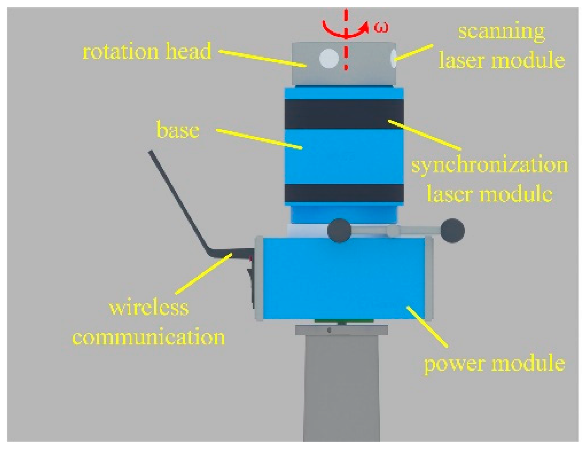
2.1. Measurement Principle

Specifically, the measurement model of wMPS can be abstracted as two rotating laser planes. The normal vectors and z-axis intercepts of two laser planes at the reference point are described as:
[ a i j b i j c i j d i j ] T
where i and j indicate the i’th transmitter and j’th laser module. They are constant after the transmitter is assembled.
When the two lasers scan across the receiver counterclockwise, the normal vectors can be expressed as:
[ a i j θ b i j θ c i j θ d i j θ ] = [ cos ( ω i t i j ) sin ( ω i t i j ) 0 0 sin ( ω i t i j ) cos ( ω i t i j ) 0 0 0 0 1 0 0 0 0 1 ] [ a i j b i j c i j d i j ]
ω i refers to the rotation speed of the i’th transmitter, and t i j refers to the time difference between the synchronization signal and j’th scanning signal.
When a laser plane scans over a receiver, the receiver will locate on the plane and the constraint formula between the laser plane and receiver can be constructed:
[ a i j θ b i j θ c i j θ d i j θ ] [ R 11 R 12 R 13 T x R 21 R 22 R 23 T y R 31 R 32 R 33 T z 0 0 0 1 ] [ x g y g z g 1 ] T = 0
R and T represent the rotation and translation components from the global coordinate system to the local coordinate system respectively. They are derived from measurement network calibration [17]. [ x g y g z g 1 ] represents the homogeneous coordinate of the receiver in the global coordinate system. There are three unknowns in the coordinate of each receiver and they will be calculable as long as more than three formulas are available. Consequently, signals from more than two transmitters with different rotation speeds will be capable for coordinate calculation. The accuracy is positively related to the number of transmitters scanning across the receiver.

2.2. Causes of Dynamic Error

As stated in Section 2.1, laser signals from at least two transmitters with different rotation speeds are necessary for coordinate calculation. For each transmitter, a receiver will obtain a synchronization pulse and two scanning pulses in sequence as shown in Figure 2. In the measuring network, the synchronization pulses from different transmitters are irrelevant in the time domain.
If the receiver is static, laser planes have a unique intersection point and the time difference between signals has no influence on measurement accuracy. However, for a moving receiver, in the period of obtaining signals from the two transmitters, i.e., t 1 to t 22 , it has been at different positions and the trajectory during that is unknown. Calculating the coordinate of the receiver directly will lead to certain dynamic error.
We define single transmitter dynamic time error δ t s _ k as the time difference between synchronization pulse and scanning pulse 1, pulse 2 ( t 1 and t 11 , t 1 and t 12 ), and the multi-transmitter dynamic error δ t m _ k is defined as the time difference between synchronization pulses from different transmitters ( t 1 and t 2 ). Note that multi-transmitter dynamic error δ t m _ k is strictly related with rotation periods and it will accumulate over rotation cycles.
δ t m _ k = mod ( N ( T k T 1 ) , T 1 )
N represents the rotation cycles and T k represents the rotation period of the transmitter k . T 1 is the rotation period of the primary transmitter in the network. δ t s _ k is determined by the distribution of two laser modules. They have an intersection angle of 90°. δ t m _ k is determined by the rotation cycles of all transmitters in the network. When the measurement network is built, it remains unchanged. δ t s _ k and δ t m _ k are uncorrelated and lead to dynamic error δ θ s _ k and δ θ m _ k in scanning angle respectively. δ θ e _ k is the static angle error and it is related with the straightness error of the laser module and centering error of the receiver. It is uncorrelated with the two error resources above. Therefore, the total dynamic error of wMPS can be expressed in Equation (5):
δ θ k = δ θ e _ k + δ θ s _ k + δ θ m _ k
The static measurement error of a single transmitter has been evaluated after it is assembled. It obeys the normal distribution and the standard deviation is about 2”. Besides, the static error at each measurement is independent and the covariance is zero. For the other two error resources, simulation experiments based on MATLAB are conducted for time error quantization.
Basing on the principle of intersection measurement, the coordinates of the receiver can be calculable if it obtains signals from two transmitters. However, there is no constraint redundancy and the accuracy and stability are relatively lower. With the increase of the transmitter amount, the accuracy will also be improved. In application, we generally construct a four-transmitter network to gain better performance. Taking it into account, a four transmitters network was built and they were in a “C” type layout, which had been tested to gain a higher accuracy than others [20]. The rotation speeds were 1600, 1800, 2000 and 2200 rev/min, respectively. A trajectory generator was applied to produce a spatial trajectory and the receiver moved along it at different speeds, i.e., 30 mm/s, 60 mm/s, and 120 mm/s. The dynamic time error δ t s _ k + δ t m _ k , i.e. the time difference between the first synchronization signal and the last scanning signal, was captured at each measurement. Experimental configuration and results are shown in Figure 3 and Figure 4:
As displayed in Figure 4, the maximum and minimum error at v = 30 mm/s are 32.24 ms and 28.06 ms. The time error corresponds to a periodic curve in the time-domain. The deviations at different speeds are lower than 0.05 ms and they are negligible in this research. Change the trajectory in subsequent simulations and we find that in the whole measurement zone the time error has great similarity with that of v = 30 mm/s. It is dependent on the rotation speeds of transmitters in the network. With the increase of rotation speeds, δ t s _ k and δ t m _ k will decrease. However, the speed and position of the receiver have little influence on dynamic time error.
In wMPS we generally set a primary transmitter. The global coordinate system will be aligned with the coordinate system of the primary transmitter. The rotation and displacement relationship between the primary transmitter and others transmitters will be calibrated during the construction of the network. Each transmitter has a certain pose and position in the global coordinate system. On the basis of the conclusion above, we divide the movement speed of the receiver into three directions: radial speed v r , tangential speed v t and axial speed v a in Figure 5. Here the radial, tangential, and axial directions mean those of each separate transmitter.
According to the transmitter model, the radial speed has little influence on the dynamic error on account of the fast light speed. Therefore, the scanning angle error caused by time error can be expressed as:
δ θ s _ k + δ θ m _ k = ( v t x 2 + y 2 + tan φ × v a x 2 + y 2 ) ( δ t s _ k + δ t m _ k )
( x y z ) is the position of the receiver in the local coordinate system. φ refers to the intersection angle between the rotation axis and laser plane. In this way, the dynamic error resources in wMPS are presented.

3. Dynamic Error Modeling and Uncertainty Analysis

3.1. Dynamic Error Modeling

In Section 2.2 we have analyzed the dynamic error mechanism. The measurement error in scanning angles causes the coordinate error of the moving receiver. The error propagation model is included in the following equations F ( P , θ ) = 0 :
{ F 1 = [ a 11 b 11 c 11 d 11 ] [ cos θ 11 sin θ 11 0 0 sin θ 11 cos θ 11 0 0 0 0 1 0 0 0 0 1 ] [ R 1 T 1 0 1 ] [ x g y g z g 1 ] T = 0 F 2 = [ a 12 b 12 c 12 d 12 ] [ cos θ 12 sin θ 12 0 0 sin θ 12 cos θ 12 0 0 0 0 1 0 0 0 0 1 ] [ R 1 T 1 0 1 ] [ x g y g z g 1 ] T = 0 F 2 n 1 = [ a n 1 b n 1 c n 1 d n 1 ] [ cos θ n 1 sin θ n 1 0 0 sin θ n 1 cos θ n 1 0 0 0 0 1 0 0 0 0 1 ] [ R n T n 0 1 ] [ x g y g z g 1 ] T = 0 F 2 n 2 = [ a n 2 b n 2 c n 2 d n 2 ] [ cos θ n 2 sin θ n 2 0 0 sin θ n 2 cos θ n 2 0 0 0 0 1 0 0 0 0 1 ] [ R n T n 0 1 ] [ x g y g z g 1 ] T = 0
The sources of coordinate uncertainty are scanning angles θ 1 , θ 2 , θ 2 n 1 , θ 2 n . They are independent of each other and generally obey the normal distribution in Figure 6. The distribution center is determined by the dynamic error and the variance is determined by the static error.
The covariance matrix θ , also seen as the input, can be expressed as:
θ = [ u 2 ( θ 1 ) 0 0 u 2 ( θ 2 n ) ]
According to the derivative rule for implicit functions [21],
d P d θ = ( d F d P ) + d F d θ
P = [ x y z 1 ] and it is the homogeneous coordinate of the receiver in the global coordinate system. d F d P and d F d θ are the Jacobian matrices of F relative to P and θ . ( d F d P ) + is the generalized inverse matrix of d F d P .
In simulations we found that the numerical stability of θ is unsatisfactory and it is highly sensitive to round-off error in programming, so the other algorithm is tried which depends on the following steps [22]:
  • Divide θ into a lower triangular matrix λ C and its transposed matrix: θ = λ C T λ C .
  • Divide d F d θ into the product of an orthogonal matrix Q C and an upper triangular matrix W C : d F d θ = Q C W C .
  • Divide d F d P into the product of a lower triangular matrix L P and an upper triangular matrix W P : d F d P = L P W P .
  • Calculate matrix M 1 through W P T M 1 = I , M = λ C W C T Q C T ( L P T ) 1 M 1 .
  • Divide M into the product of an orthogonal matrix Q M and an upper triangular matrix R M : M = Q M W M .
  • Describe the uncertainty u x y z as: u x y z = u P = W M T W M .

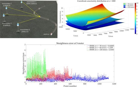
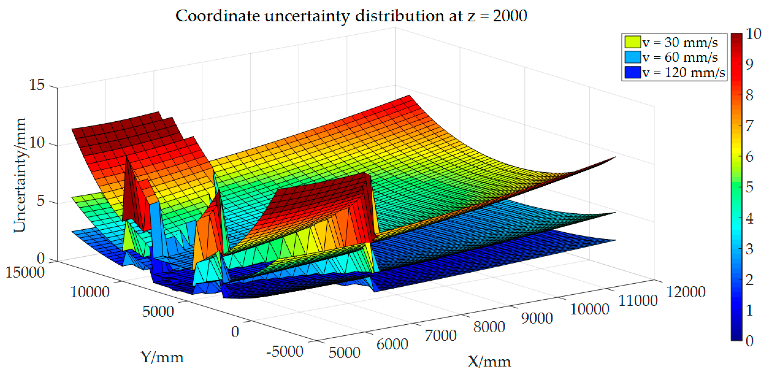
3.2. Uncertainty Simulation and Analysis

Basing on the mathematical solution in Section 3.1, simulation experiments were carried out in MATLAB. A measurement network with four transmitters was built and the layout was the same as Section 2.2. A receiver moved at different speeds, 30, 60, and 120 mm/s respectively. We set 4800 points at three horizontal planes (z = 0, z = 1000, and z = 2000) uniformly as Figure 7. The coordinate uncertainty components of each point, i.e., u x , u y and u z , were calculated. In Figure 8, Figure 9 and Figure 10 we have displayed the compound uncertainty u which indicates the distance between the theoretical point and measurement result.
u = u x 2 + u y 2 + u z 2
We can draw a conclusion from Figure 8, Figure 9 and Figure 10 that the dynamic error is in a linear relationship with the movement speed of the receiver. With the increase of receiver speed, the dynamic error will also get larger. Although in all cases it contains a constant static error, it occupies a small part in the total dynamic error. The single transmitter dynamic error and multi-transmitter dynamic error are dominating. Moreover, the layout of the network also influences the dynamic error. The optimal intersection angle for measurement is 110°. In the margin area, where the intersection angle is extremely small, the measurement error may be enlarged, which has the same characteristics as static conditions [20].

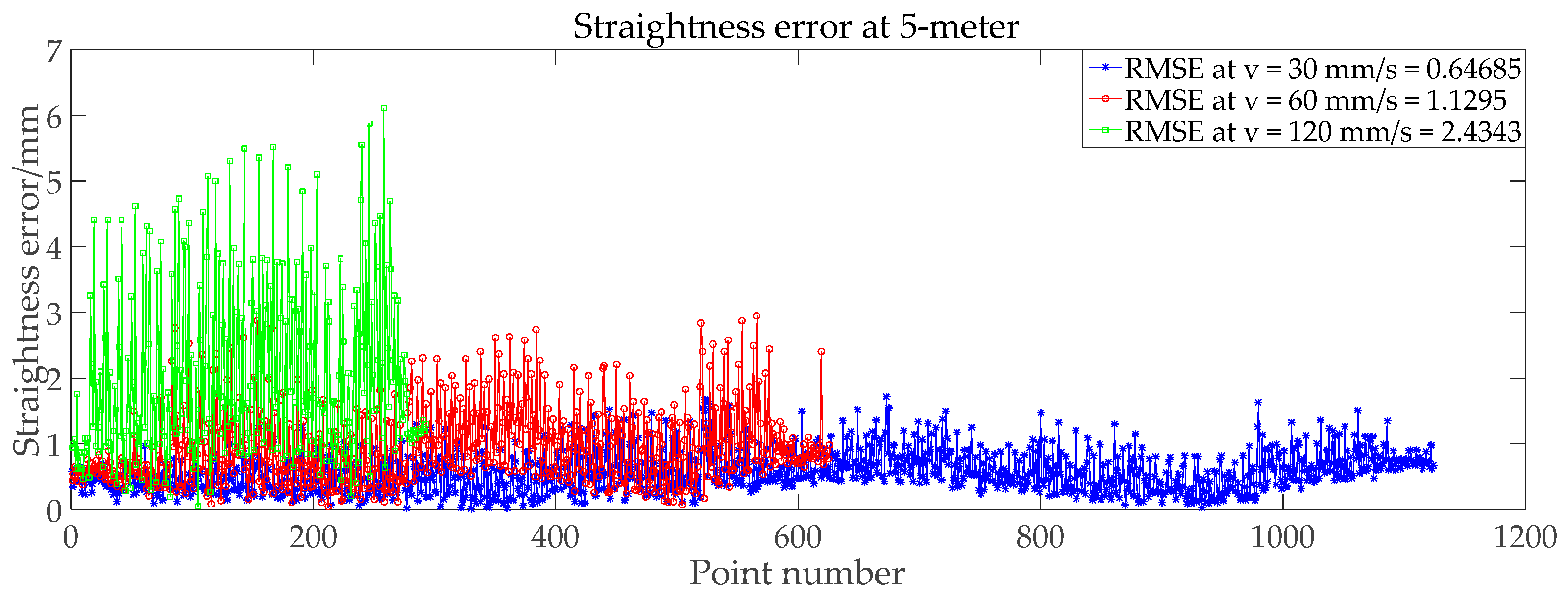
4. Experimental Verification

To verify the mathematic model of wMPS dynamic error, practical experiments are designed and the configuration is displayed in Figure 11:
We first constructed a measurement network with four transmitters. The rotation speeds of transmitters were set as 1600, 1800, 2000, and 2200 rev/min respectively. They were consistent with those in simulations in Section 2.2. The orientation parameter of transmitters was calibrated according to a coordinate control network [17]. A linear guide with a maximum travel distance of 800 mm was applied to generate a standard linear trajectory and its straightness error was better than 0.07 mm after calibration with an interferometer. It is much smaller than dynamic error and the linear guide can be seen as a reference in experiments. A receiver was located on the platform and moves with it synchronously. Movement speeds were set as 30 mm/s, 60 mm/s, and 120 m/s respectively. Experiments were carried out in two conditions successively: the linear guide was 5 m/7 m in front of the primary transmitter. To break the specificity in speed direction, in both conditions the linear guide had a horizontal angle of 45° and a vertical angle of 20° in the global coordinate system.
The real-time coordinates of the receiver during each motion were recorded. Then we fitted a spatial line. The dynamic error was evaluated by the straightness error and the root-mean-square errors at each case were also calculated in Figure 12 and Figure 13.
For further comparison, Table 1 lists the deviations between practical experiment results and corresponding simulation results. We can see that the experimental results match with the simulation results, and the maximum deviation between them is 0.091 mm. The dynamic error model of wMPS is validated to be reasonable.

5. Conclusions

Dynamic coordinate measurement in industrial manufacturing is a popular issue which needs to be solved urgently. wMPS is now recognized as a promising solution because of its great potential. Nevertheless, the dynamic error caused by measurement principle gains little research and limits its further development. In this article, we first analyzed the mechanism of dynamic error. Then error modeling and simulations experiments about the uncertainty were carried out. The characteristics of the dynamic error were expounded. To validate the mathematical model, practical experiments were done and the results matched well with simulations. It laid the foundation for error compensation and performance improvement. It is noteworthy that we have made an assumption that the receiver moves at a constant speed. As stated in Section 1, wMPS has a measurement frequency of 20 Hz. It is often used in industrial manufacturing such as aircraft assembly and leveling, digital shipbuilding, and tooling monitoring. There is often no jump in acceleration for moving targets on such occasions. In a measurement cycle, i.e., 50 ms, the speed of the target can be seen as constant. The assumption is acceptable in practice.
In the future, we will focus our research on error compensation through hardware and software enhancement. The inertial measurement unit (IMU) can sense its own acceleration at a frequency of 400 Hz (such as STIM 300) and it will be embedded in the receiver. At each measurement cycle, the IMU will provide the real-time speed of the receiver. The model may be further optimized. Besides, the rotation speed of the transmitter has a great influence on the dynamic error. We will try more advanced shaft system and improve the rotation speed, which can also ensure a longer working life. As for software, a model-based compensation algorithm may be a good choice for dynamic error restriction. The development of machine learning provides novel ideas for our future work.

Author Contributions

Conceptualization, methodology, experiment design, and original draft, S.S. and L.Y.; experiment and analysis, R.D. and Z.Z.; software, J.L.; supervision and funding acquisition, J.Z. and C.L.; review and editing, S.S.

Funding

This research was funded by the National Key Research and Development Program of China, Grant No. 2017YFF0204802; National Natural Science Foundation of China, Grant Nos. 51721003, 51775380, 51705023 and Natural Science Foundation of Tianjin, Grant No. 16JCZDJC38100.

Conflicts of Interest

The authors declare no conflict of interest.

References

  1. Zhou, K.L.; Liu, T.G.; Zhou, L.F. Industry 4.0: Towards future industrial opportunities and challenges. In Proceedings of the 12th International Conference on Fuzzy Systems and Knowledge Discovery (FSKD), Zhangjiajie, China, 15–17 August 2015; pp. 2147–2152. [Google Scholar]
  2. Zhong, R.Y.; Xu, X.; Klotz, E.; Newman, S.T. Intelligent manufacturing in the context of industry 4.0: A review. Engineering 2017, 3, 616–630. [Google Scholar] [CrossRef]
  3. Schmitt, R.H.; Peterek, M.; Morse, E.; Knapp, W.; Galetto, M.; Hartig, F.; Goch, G.; Hughes, B.; Forbes, A.; Estler, W.T. Advances in large-scale metrology—Review and future trends. CIRP Ann. 2016, 65, 643–665. [Google Scholar] [CrossRef]
  4. Muralikrishnan, B.; Phillips, S.; Sawyer, D. Laser trackers for large-scale dimensional metrology: A review. Precis. Eng. J. Int. Soc. Precis. Eng. Nanotechnol. 2016, 44, 13–28. [Google Scholar] [CrossRef]
  5. Franceschini, F.; Galetto, M.; Maisano, D.; Mastrogiacomo, L. Large-scale dimensional metrology (LSDM): From tapes and theodolites to multi-sensor systems. Precis. Eng. 2014, 15, 1739–1758. [Google Scholar] [CrossRef]
  6. Aguado, S.; Santolaria, J.; Samper, D.; Velazquez, J.; Javierre, C.; Fernandez, A. Adequacy of technical and commercial alternatives applied to machine tool verification using laser tracker. Appl. Sci. 2016, 6, 16. [Google Scholar] [CrossRef]
  7. Wang, Z.; Maropolous, P.G. Real-time error compensation of a three-axis machine tool using a laser tracker. Int. J. Adv. Manuf. Technol. 2013, 69, 919–933. [Google Scholar] [CrossRef]
  8. Muralikrishnan, B.; Lee, V.; Blackburn, C.; Sawyer, D.; Phillips, S.; Ren, W.; Hughes, B. Assessing ranging errors as a function of azimuth in laser trackers and tracers. Meas. Sci. Technol. 2013, 24, 6. [Google Scholar] [CrossRef]
  9. Hughes, B.; Forbes, A.; Lewis, A.; Sun, W.; Veal, D.; Nasr, K. Laser tracker error determination using a network measurement. Meas. Sci. Technol. 2011, 22, 12. [Google Scholar] [CrossRef]
  10. Luhmann, T. Close range photogrammetry for industrial applications. ISPRS J. Photogramm. Remote Sens. 2010, 65, 558–569. [Google Scholar] [CrossRef]
  11. Sun, B.; Zhu, J.G.; Yang, L.H.; Yang, S.R.; Guo, Y. Sensor for in-motion continuous 3d shape measurement based on dual line-scan cameras. Sensors 2016, 16, 15. [Google Scholar] [CrossRef] [PubMed]
  12. Jung, K.; Kim, S.; Im, S.; Choi, T.; Chang, M. A photometric stereo using re-projected images for active stereo vision system. Appl. Sci. 2017, 7, 10. [Google Scholar] [CrossRef]
  13. Montironi, M.A.; Castellini, P.; Stroppa, L.; Paone, N. Adaptive autonomous positioning of a robot vision system: Application to quality control on production lines. Robot. Comput. Integr. Manuf. 2014, 30, 489–498. [Google Scholar] [CrossRef]
  14. Huang, S.R.; Shinya, K.; Bergstrom, N.; Yamakawa, Y.; Yamazaki, T.; Ishikawa, M. Dynamic compensation robot with a new high-speed vision system for flexible manufacturing. Int. J. Adv. Manuf. Technol. 2018, 95, 4523–4533. [Google Scholar] [CrossRef]
  15. Di Leo, G.; Liguori, C.; Pietrosanto, A.; Sommella, P. A vision system for the online quality monitoring of industrial manufacturing. Opt. Lasers Eng. 2017, 89, 162–168. [Google Scholar] [CrossRef]
  16. Liu, T.; Yin, S.B.; Guo, Y.; Zhu, J.G. Rapid global calibration technology for hybrid visual inspection system. Sensors 2017, 17, 16. [Google Scholar] [CrossRef] [PubMed]
  17. Zhao, Z.Y.; Zhu, J.G.; Lin, J.R.; Yang, L.H.; Xue, B.; Xiong, Z. Transmitter parameter calibration of the workspace measurement and positioning system by using precise three-dimensional coordinate control network. Opt. Eng. 2014, 53, 8. [Google Scholar] [CrossRef]
  18. Guo, F.Y.; Wang, Z.Q.; Kang, Y.G.; Li, X.N.; Chang, Z.P.; Wang, B.B. Positioning method and assembly precision for aircraft wing skin. Proc. Inst. Mech. Eng. Part B J. Eng. Manuf. 2018, 232, 317–327. [Google Scholar] [CrossRef]
  19. Mei, Z.Y.; Maropoulos, P.G. Review of the application of flexible, measurement-assisted assembly technology in aircraft manufacturing. Proc. Inst. Mech. Eng. Part B J. Eng. Manuf. 2014, 228, 1185–1197. [Google Scholar] [CrossRef]
  20. Guo, S.Y.; Lin, J.R.; Ren, Y.J.; Yang, L.H.; Zhu, J.G. Study of network topology effect on measurement accuracy for a distributed rotary-laser measurement system. Opt. Eng. 2017, 56, 8. [Google Scholar] [CrossRef]
  21. Golub, G.H.; Van Loan, C.F. Matrix Computations, 4th ed.; The John Hopkins University Press: Baltimore, MD, USA, 2012; pp. 63–105. [Google Scholar]
  22. Joint Committee for Guides in Metrology. Evaluation of Measurement Data—Supplement 2 to the “Guide to the Expression of Uncertainty in Measurement”—Extension to Any Number of Output Quantities; Joint Committee for Guides in Metrology: Paris, France, 2011. [Google Scholar]
Figure 1. Transmitter configuration.
Applsci 09 00062 g001
Figure 2. Time sequence of signals from two transmitters.
Applsci 09 00062 g002
Figure 3. Configuration of simulation experiments.
Applsci 09 00062 g003
Figure 4. Dynamic time error in the four-transmitter network.
Applsci 09 00062 g004
Figure 5. Transmitter model and speed decomposition.
Applsci 09 00062 g005
Figure 6. Scanning angle error distribution.
Applsci 09 00062 g006
Figure 7. Points distribution in the measurement zone.
Applsci 09 00062 g007
Figure 8. Coordinate uncertainty distribution of points at z = 0.
Applsci 09 00062 g008
Figure 9. Coordinate uncertainty distribution of points at z = 1000.
Applsci 09 00062 g009
Figure 10. Coordinate uncertainty distribution of points at z = 2000.
Applsci 09 00062 g010
Figure 11. Experiment configuration: (a) Overview; (b) linear guide and receiver.
Applsci 09 00062 g011
Figure 12. Straightness error of practical trajectory at 5-m at different speeds.
Applsci 09 00062 g012
Figure 13. Straightness error of practical trajectory at 7-m at different speeds.
Applsci 09 00062 g013
Table 1. Deviation between simulation and practical experiments.
Straightness Error/mm
Simulation ExperimentsPractical ExperimentsDeviation
5 m7 m5 m7 m
v = 30 mm/s0.6350.8290.6470.9060.0120.077
v = 60 mm/s1.0821.6271.1301.6930.0480.066
v = 120 mm/s2.3523.0702.4343.1610.0820.091

