Seismic Response of Steel Moment Frames (SMFs) Considering Simultaneous Excitations of Vertical and Horizontal Components, Including Fling-Step Ground Motions


Abstract
:1. Introduction
2. The Effects and Characteristics of Near-Field Earthquakes
- (1)
- The velocity and acceleration history of these earthquakes have long-period pulses.
- (2)
- The ratio of maximum velocity to the maximum acceleration of ground is significant in these earthquakes.
- (3)
- Sometimes near-field quakes lead to major permanent transformations of the earth [31].
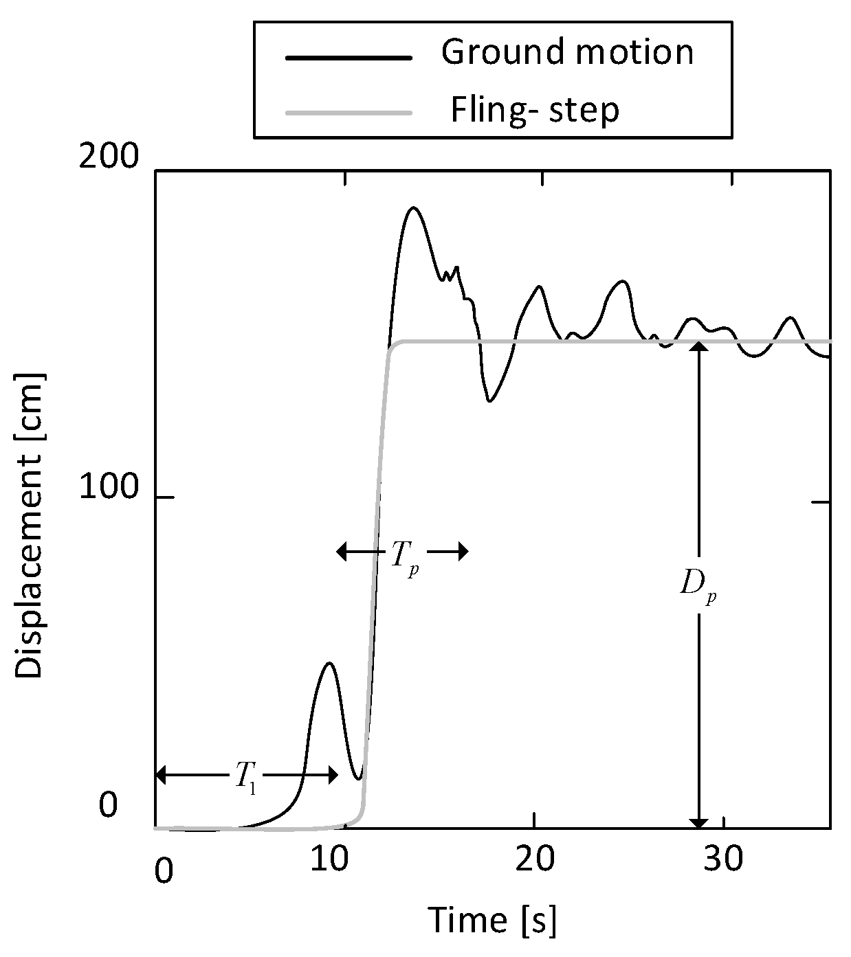
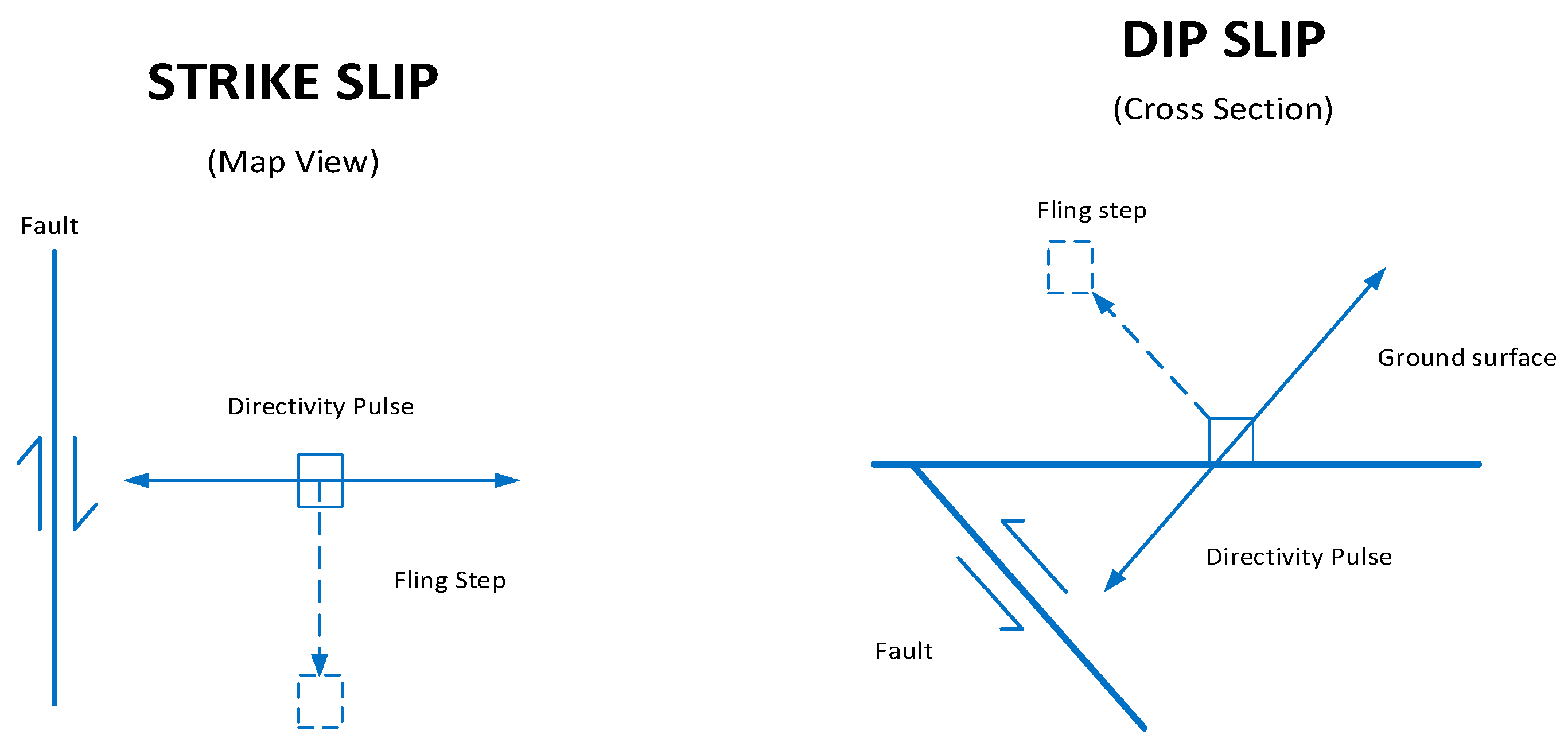
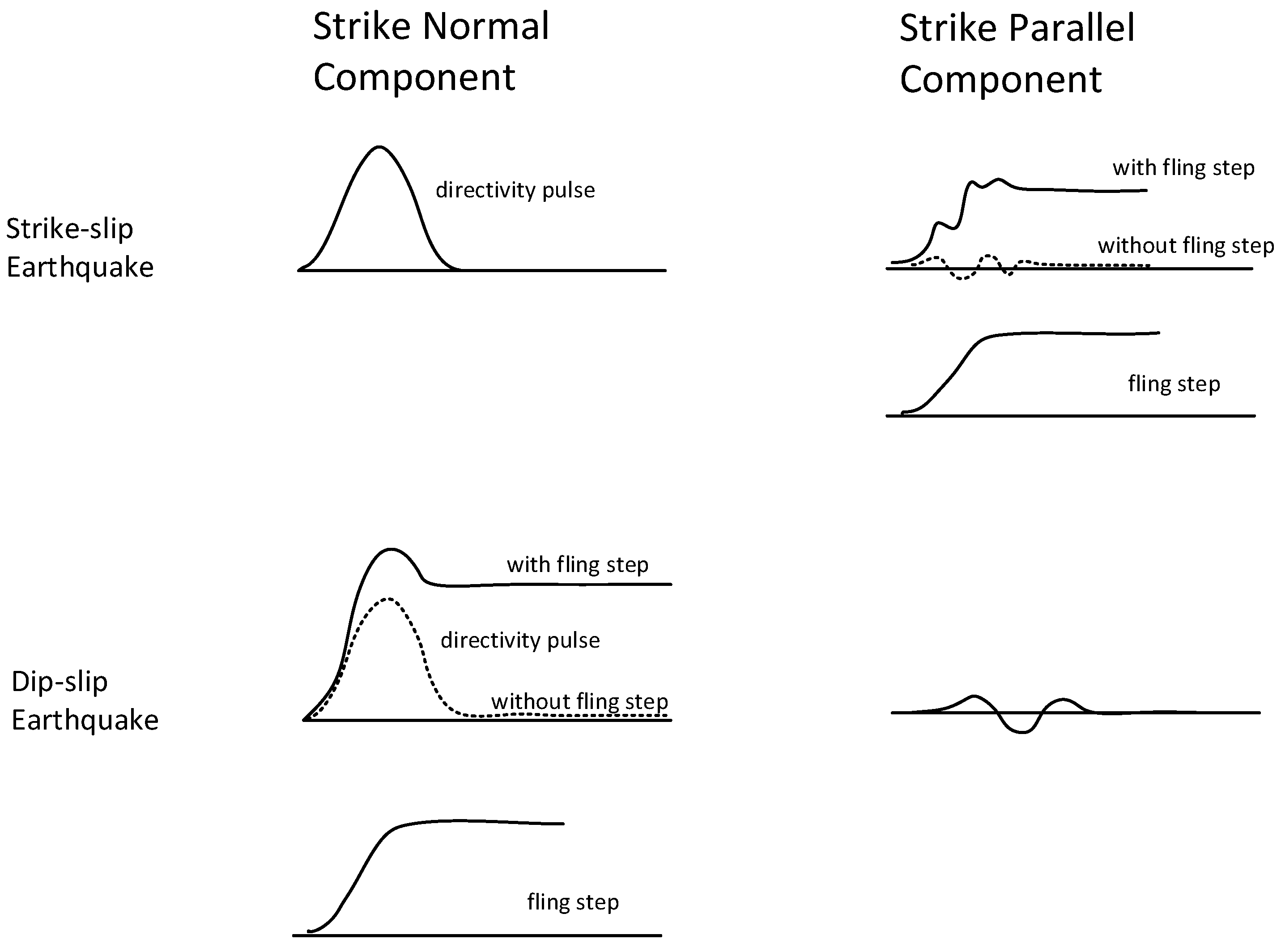
Fling-Step Effect
3. Numerical Models
3.1. Selected Numerical Models
3.2. Records Selection
4. Evaluating the Seismic Response of Structures
5. Conclusions
Author Contributions
Funding
Conflicts of Interest
References
- Bolt, B.A.; Abrahamson, N.A. 59 Estimation of strong seismic ground motions. Int. Geophys. 2003, 81, 983–1001. [Google Scholar] [CrossRef]
- Ventura, C.E.; Archila, M.; Bebamzadeh, A.; Liam Finn, W.D. Large coseismic displacements and tall buildings. Struct. Des. Tall Spec. Build. 2011, 20, S85–S99. [Google Scholar] [CrossRef]
- Grimaz, S.; Malisan, P. Near field domain effects and their consideration in the international and Italian seismic codes. Boll. Geofis. Teor. Appl. 2014, 55, 717–738. [Google Scholar] [CrossRef]
- Avossa, A.M.; Pianese, G. Damping effects on the seismic response of base-isolated structures with LRB devices. Ing. Sismica 2017, 34, 3–29. [Google Scholar]
- Carydis, P.; Lekkas, E. The Haiti Earthquake Mw = 7.0 of January 12 th 2010: Structural and geotechnical engineering field observations, near-field ground motion estimation and interpretation of the damage to buildings and infrastructure in the Port-au-Prince area. Ing. Sismica 2011, 28, 24–42. [Google Scholar]
- Bhandari, M.; Bharti, S.D.; Shrimali, M.K.; Datta, T.K. Seismic Fragility Analysis of Base-Isolated Building Frames Excited by Near- and Far-Field Earthquakes. J. Perform. Constr. Facil. 2019, 33. [Google Scholar] [CrossRef]
- Tajammolian, H.; Khoshnoudian, F.; Talaei, S.; Loghman, V. The effects of peak ground velocity of near-field ground motions on the seismic responses of base-isolated structures mounted on friction bearings. Earthq. Struct. 2014, 7, 1159–1282. [Google Scholar] [CrossRef]
- Kalkan, E.; Kunnath, S.K. Effects of fling step and forward directivity on seismic response of buildings. Earthq. Spectra 2006, 22, 367–390. [Google Scholar] [CrossRef]
- Mavroeidis, G.P.; Dong, G.; Papageorgiou, A.S. Near-fault ground motions, and the response of elastic and inelastic single-degree-of-freedom (SDOF) systems. Earthq. Eng. Struct. Dyn. 2004, 33, 1023–1049. [Google Scholar] [CrossRef]
- Somerville, P.G.; Smith, N.F.; Graves, R.W.; Abrahamson, N.A. Modification of empirical strong ground motion attenuation relations to include the amplitude and duration effects of rupture directivity. Seismol. Res. Lett. 1997, 68, 199–222. [Google Scholar] [CrossRef]
- Baker, J.W. Identification of near-fault velocity pulses and prediction of resulting response spectra. In Proceedings of the Geotechnical Earthquake Engineering and Soil Dynamics IV, Sacramento, CA, USA, 18–22 May 2008. [Google Scholar]
- Akkar, S.; Yazgan, U.; Gülkan, P. Drift estimates in frame buildings subjected to near-fault ground motions. J. Struct. Eng. 2005, 131, 1014–1024. [Google Scholar] [CrossRef]
- MacRae, G.A.; Morrow, D.V.; Roeder, C.W. Near-fault ground motion effects on simple structures. J. Struct. Eng. 2001, 127, 996–1004. [Google Scholar] [CrossRef]
- Malhotra, P.K. Response of buildings to near-field pulse-like ground motions. Earthq. Eng. Struct. Dyn. 1999, 28, 1309–1326. [Google Scholar] [CrossRef]
- Wong, K.K.F.; Yang, R. Comparing response of SDF systems to near-fault and far-fault earthquake motions in the context of spectral regions. Earthq. Eng. Struct. Dyn. 2001, 30, 1769–1789. [Google Scholar] [CrossRef]
- Mohseni, I.; Lashkariani, H.A.; Kang, J.; Kang, T.H.K. Dynamic response evaluation of long-span reinforced arch bridges subjected to near- and far-field ground motions. Appl. Sci. 2018, 8, 1243. [Google Scholar] [CrossRef]
- Zhao, D.; Liu, Y.; Li, H. Self-tuning fuzzy control for seismic protection of smart base-isolated buildings subjected to pulse-type near-fault earthquakes. Appl. Sci. 2017, 7, 1185. [Google Scholar] [CrossRef]
- Gillie, J.L.; Rodriguez-Marek, A.; McDaniel, C. Strength reduction factors for near-fault forward-directivity ground motions. Eng. Struct. 2010, 32, 273–285. [Google Scholar] [CrossRef]
- Jalali, R.S.; Trifunac, M.D. A note on strength-reduction factors for design of structures near earthquake faults. Soil Dyn. Earthq. Eng. 2008, 28, 212–222. [Google Scholar] [CrossRef]
- Burks, L.S.; Baker, J.W. A predictive model for fling-step in near-fault ground motions based on recordings and simulations. Soil Dyn. Earthq. Eng. 2016, 80, 119–126. [Google Scholar] [CrossRef]
- Farid Ghahari, S.; Jahankhah, H.; Ghannad, M.A. Study on elastic response of structures to near-fault ground motions through record decomposition. Soil Dyn. Earthq. Eng. 2010, 30, 536–546. [Google Scholar] [CrossRef]
- Shahbazi, S.; Khatibinia, M.; Mansouri, I.; Hu, J.W. Seismic evaluation of special steel moment frames undergoing near-field earthquakes with forward directivity by considering soil-structure interaction effects. Sci. Iran. 2018. [Google Scholar] [CrossRef]
- Nastri, E.; D’Aniello, M.; Zimbru, M.; Streppone, S.; Landolfo, R.; Montuori, R.; Piluso, V. Seismic response of steel Moment Resisting Frames equipped with friction beam-to-column joints. Soil Dyn. Earthq. Eng. 2019, 119, 144–157. [Google Scholar] [CrossRef]
- Dell’Aglio, G.; Montuori, R.; Nastri, E.; Piluso, V. Consideration of second-order effects on plastic design of steel moment resisting frames. Bull. Earthq. Eng. 2019. [Google Scholar] [CrossRef]
- Piluso, V.; Pisapia, A.; Castaldo, P.; Nastri, E. Probabilistic Theory of Plastic Mechanism Control for Steel Moment Resisting Frames. Struct. Saf. 2019, 76, 95–107. [Google Scholar] [CrossRef]
- Mansouri, I.; Shahbazi, S.; Hu, J.W.; Arian Moghaddam, S. Effects of pulse-like nature of forward directivity ground motions on the seismic behavior of steel moment frames. Earthq. Struct. 2019, in press. [Google Scholar]
- Sánchez-Olivares, G.; Tomás Espín, A. Design of planar semi-rigid steel frames using genetic algorithms and Component Method. J. Constr. Steel Research. 2013, 88, 267–278. [Google Scholar] [CrossRef]
- Macedo, L.; Silva, A.; Castro, J.M. A more rational selection of the behaviour factor for seismic design according to Eurocode 8. Eng. Struct. 2019, 188, 69–86. [Google Scholar] [CrossRef]
- Mansouri, I.; Saffari, H. A new steel panel zone model including axial force for thin to thick column flanges. Steel Compos. Struct. 2014, 16, 417–436. [Google Scholar] [CrossRef]
- Saffari, H.; Mansouri, I.; Bagheripour, M.H.; Dehghani, H. Elasto-plastic analysis of steel plane frames using Homotopy Perturbation Method. J. Constr. Steel Research. 2012, 70, 350–357. [Google Scholar] [CrossRef]
- Li, S.; Xie, L.L. Progress and trend on near-field problems in civil engineering. Acta Seismol. Sin. 2007, 20, 105–114. [Google Scholar] [CrossRef]
- Stewart, J.P.; Chiou, S.J.; Bray, J.D.; Graves, R.W.; Somerville, P.G.; Abrahamson, N.A. Ground Motion Evaluation Procedures for Performance-Based Design; PEER Report 2001/09; Pacific Earthquake Engineering Research Center, University of California Berkeley: Berkeley, CA, USA, 2001. [Google Scholar]
- Kalkan, E.; Adalier, K.; Pamuk, A. Near source effects and engineering implications of recent earthquakes in Turkey. In Proceedings of the 5th international conference on case histories in geotechnical engineering, New York, NY, USA, 13–17 April 2004. [Google Scholar]
- Standard2800. In Iranian Code of Practice for Seismic Resistant Design of Buildings, 4th ed.; Building and Housing Research Center: Tehran, Iran, 2014.
- Etemadi Mashhadi, M.R. Development of Fragility Curves for Seismic Assessment of Steel Structures with Consideration of Soil-Structure Interaction. Master’s Thesis, University of Birjand, Birjand, Iran, 2015. [Google Scholar]
- Shahbazi, S.; Mansouri, I.; Hu, J.W.; Sam Daliri, N.; Karami, A. Seismic response of steel SMFs subjected to vertical components of far- and near-field earthquakes with forward directivity effects. Adv. Civ. Eng. 2019, 2019, 2647387. [Google Scholar] [CrossRef]
- Shahbazi, S.; Mansouri, I.; Hu, J.W.; Karami, A. Effect of soil classification on seismic behavior of SMFs considering soil-structure interaction and near-field earthquakes. Shock Vib. 2018, 2018, 4193469. [Google Scholar] [CrossRef]
- Lignos, D.G.; Krawinkler, H. Sidesway Collapse of Deteriorating Structural Systems under Seismic Excitations; Rep. No. 172; John A. Blume Earthquake Engineering Center, Stanford University: Stanford, CA, USA, 2009. [Google Scholar]
- Gupta, A.; Krawinkler, H. Seismic Demands for Performance Evaluation of Steel Moment Resisting Frame Structures; Rep. No. 132; John A. Blume Earthquake Engineering Center, Stanford University: Stanford, CA, USA, 1999. [Google Scholar]
- OpenSees. Open System for Earthquake Engineering Simulation. Available online: http://opensees.berkeley.edu:PEER (accessed on 16 May 2019).
- Ibarra, L.F.; Krawinkler, H. Global Collapse of Frame Structures under Seismic Excitations; Rep. No. 152; John A. Blume Earthquake Engineering Center, Stanford University: Stanford, CA, USA, 2005. [Google Scholar]


| No. | Column | Beam | No. | Column | Beam | ||
|---|---|---|---|---|---|---|---|
| 3-story | 1 | Box 200 × 200 × 20 | IPE 300 | 8-story | 1 | Box 280 × 280 × 20 | IPE 400 |
| 2 | Box 200 × 200 × 20 | IPE 300 | 2 | Box 280 × 280 × 20 | IPE 400 | ||
| 3 | Box 200 × 200 × 20 | IPE 270 | 3 | Box 240 × 240 × 20 | IPE 360 | ||
| 4 | Box 280 × 280 × 20 | IPE 400 | 4 | Box 180 × 180 × 20 | IPE 330 | ||
| 5 | Box 280 × 280 × 20 | IPE 300 | 5 | Box 400 × 400 × 20 | IPE 400 | ||
| 6 | Box 280 × 280 × 20 | IPE 270 | 6 | Box 340 × 340 × 20 | IPE 450 | ||
| 5-story | 1 | Box 240 × 240 × 20 | IPE 330 | 7 | Box 300 × 300 × 20 | IPE 400 | |
| 2 | Box 240 × 240 × 20 | IPE 360 | 8 | Box 240 × 240 × 20 | IPE 360 | ||
| 3 | Box 180 × 180 × 20 | IPE 240 | |||||
| 4 | Box 300 × 300 × 20 | IPE 330 | |||||
| 5 | Box 300 × 300 × 20 | IPE 360 | |||||
| 6 | Box 240 × 240 × 20 | IPE 240 |
| No | #Earthquakes | Year | Event | Mech a | Station | Comp | Site Class | Mw | PGA (g) | PGV (cm/s) | PGD (cm) | Fling Disp. (cm) |
|---|---|---|---|---|---|---|---|---|---|---|---|---|
| (a) Far-Field Recordings Vertical | ||||||||||||
| 1 | #EQFV1 | 1992 | Big Bear | SS | Desert Hot Spr. | 90 | Soil | 6.4 | 0.11 | 10 | 1.21 | - |
| 2 | #EQFV2 | 1952 | Kern County | TH/REV | Taft | 111 | Soil | 7.5 | 0.11 | 7 | 5.76 | - |
| 3 | #EQFV3 | 1989 | Loma Prieta | OB | Cliff House | 90 | Stiff Soil | 7.0 | 0.06 | 0.07 | 1.43 | - |
| (b) Far-Field Recordings Horizontal | ||||||||||||
| 1 | #EQFH1 | 1992 | Big Bear | SS | Desert Hot Spr. | 90 | Soil | 6.4 | 0.23 | 19.14 | 4.53 | - |
| 2 | #EQFH2 | 1952 | Kern County | TH/REV | Taft | 111 | Soil | 7.5 | 0.18 | 17.50 | 8.79 | - |
| 3 | #EQFH3 | 1989 | Loma Prieta | OB | Cliff House | 90 | Stiff Soil | 7.0 | 0.11 | 19.79 | 5.02 | - |
| (c) Near-Field Recordings (Fling-step) Horizontal | ||||||||||||
| 1 | #EQNH1 | 1999 | Chi-Chi | TH | TCU084 | NS | Soil | 7.6 | 0.42 | 42.63 | 64.91 | 59.43 |
| 2 | #EQNH2 | 1999 | Chi-Chi | TH | TCU052 | NS | Soil | 7.6 | 0.44 | 216 | 709.09 | 697.12 |
| 3 | #EQNH3 | 1999 | Chi-Chi | TH | TCU0129 | NS | Soil | 7.6 | 0.61 | 54.56 | 82.70 | 67.54 |
| (d) Near-Field Recordings (Fling-step) Vertical | ||||||||||||
| 1 | #EQNV1 | 1999 | Chi-Chi | TH | TCU084 | NS | Soil | 7.6 | 0.32 | 25 | 13.24 | - |
| 2 | #EQNV2 | 1999 | Chi-Chi | TH | TCU052 | NS | Soil | 7.6 | 0.34 | 38.8 | 24.39 | - |
| 3 | #EQNV3 | 1999 | Chi-Chi | TH | TCU0129 | NS | Soil | 7.6 | 0.19 | 24.4 | 154 | - |
| (e) Near-Field Recordings (Non Fling-step) | ||||||||||||
| 1 | #EQN1 | 1989 | Loma Prieta | OB | LGPC | 00 | Stiff Soil | 7.0 | 0.56 | 94.81 | 41.13 | - |
| 2 | #EQN2 | 1994 | Northridge | TH | Olive view | 360 | Soil | 6.7 | 0.84 | 130.37 | 31.72 | - |
| 3 | #EQN3 | 1992 | Cape Mendocino | TH | Petrolia | 90 | Stiff Soil | 7.1 | 0.66 | 90.16 | 28.89 | - |
| Story | Field | Inter-Story Drift Ratio (Max)Ave | Near/Far | DisplacementAve (m) | Near/Far |
|---|---|---|---|---|---|
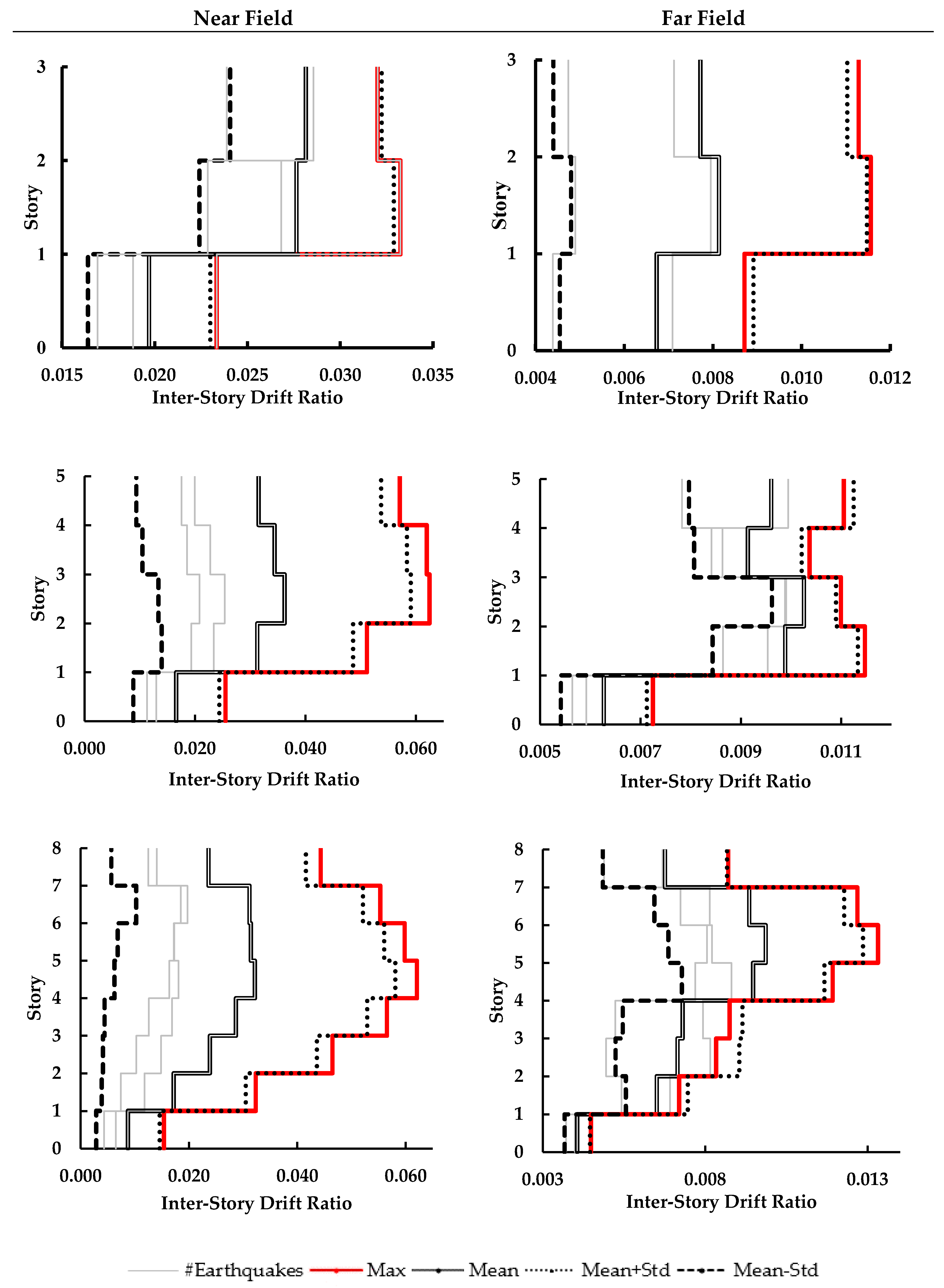
| 3 | Near | 0.03 | 3 | 0.23 | 3.29 |
| Far | 0.01 | 0.07 | |||
| 5 | Near | 0.04 | 4 | 0.47 | 3.36 |
| Far | 0.01 | 0.14 | |||
| 8 | Near | 0.03 | 3 | 0.58 | 3.41 |
| Far | 0.01 | 0.17 | |||
| Axial ForceAve (kN) | MomentAve (kN·m) | ||||
| 3 | Near | 500.8 | 2.16 | 552.7 | 2.64 |
| Far | 232.1 | 209.5 | |||
| 5 | Near | 1173.5 | 1.75 | 1078.2 | 2.35 |
| Far | 672.6 | 458.3 | |||
| 8 | Near | 2250.9 | 1.55 | 1376.1 | 1.9 |
| Far | 1448 | 723.1 | |||
| AccelerationAve (m/s2) | VelocityAve (m/s) | ||||
| 3 | Near | 17.76 | 2.09 | 1.42 | 2.12 |
| Far | 8.48 | 0.67 | |||
| 5 | Near | 18.57 | 1.74 | 2.06 | 1.93 |
| Far | 10.67 | 1.07 | |||
| 8 | Near | 20.48 | 2.02 | 2.39 | 2.06 |
| Far | 10.15 | 1.16 |
| Field | Story ShearAve (kN) | Near/Far | |
|---|---|---|---|
| 3 | Near | 3856.2 | 1.37 |
| Far | 2816.4 | ||
| 5 | Near | 11,288.9 | 1.47 |
| Far | 7704.8 | ||
| 8 | Near | 35,543.9 | 1.68 |
| Far | 21,204.1 |
| Story | Near Field | Inter-Story Drift Ratio (Max)Ave | F-S/Non F-S | DisplacementAve (m) | F-S/Non F-S |
|---|---|---|---|---|---|
| 3 | F-S (fling-step) | 0.03 | 0.75 | 0.23 | 0.68 |
| Non-F-S | 0.04 | 0.34 | |||
| (Non-fling-step) | |||||
| 5 | F-S | 0.04 | 0.8 | 0.47 | 0.89 |
| Non-F-S | 0.05 | 0.53 | |||
| 8 | F-S | 0.03 | 0.75 | 0.58 | 0.92 |
| Non-F-S | 0.04 | 0.63 | |||
| Axial ForceAve (kN) | MomentAve (kN·m) | ||||
| 3 | F-S | 500.8 | 0.78 | 552.7 | 0.83 |
| Non-F-S | 638.26 | 663.72 | |||
| 5 | F-S | 1173.5 | 0.82 | 1078.2 | 0.89 |
| Non-F-S | 1427.43 | 1210.37 | |||
| 8 | F-S | 2250.9 | 0.86 | 1376.1 | 0.79 |
| Non-F-S | 2618.67 | 1734.04 | |||
| AccelerationAve (m/s2) | VelocityAve (m/s) | ||||
| 3 | F-S | 17.76 | 0.65 | 1.42 | 0.55 |
| Non-F-S | 27.28 | 2.56 | |||
| 5 | F-S | 18.57 | 0.69 | 2.06 | 0.75 |
| Non-F-S | 26.84 | 2.75 | |||
| 8 | F-S | 20.48 | 0.8 | 2.39 | 0.89 |
| Non-F-S | 25.46 | 2.68 |
| Near Field | Story shearAve (kN) | F-S/Non F-S | |
|---|---|---|---|
| 3 | F-S | 3856.2 | 2.28 |
| Non-F-S | 1693.12 | ||
| 5 | F-S | 11,288.9 | 2.66 |
| Non-F-S | 4243.55 | ||
| 8 | F-S | 35,543.9 | 3.11 |
| Non-F-S | 11,412.65 |
| No. Story | Max Inter-Story Drift Ratio | Max Displacement (m) | Max Acceleration (m/s2) | Max Velocity (m/s) | Max Column Axial Force (kN) | Max Story shear (kN) | Max Moment Force (kN·m) | ||||||||||||||
|---|---|---|---|---|---|---|---|---|---|---|---|---|---|---|---|---|---|---|---|---|---|
| FF | NF | Ratio | FF | NF | Ratio | FF | NF | Ratio | FF | NF | Ratio | FF | NF | Ratio | FF | NF | Ratio | FF | NF | Ratio | |
| 3 | 0.01 | 0.03 | 3 | 0.10 | 0.28 | 2.80 | 10.86 | 28.41 | 2.62 | 0.90 | 1.56 | 1.73 | 294.43 | 580.12 | 1.97 | 2777.89 | 3347.99 | 1.21 | 265.49 | 614.71 | 2.32 |
| 5 | 0.01 | 0.06 | 6 | 0.14 | 0.82 | 5.86 | 12.65 | 19.53 | 1.54 | 1.18 | 2.51 | 2.13 | 712.57 | 147,438.80 | 2.07 | 6183.12 | 8786.29 | 1.42 | 522.48 | 1578.54 | 3.02 |
| 8 | 0.01 | 0.06 | 6 | 0.21 | 1.15 | 5.48 | 12.08 | 23.20 | 1.92 | 1.40 | 3.56 | 2.54 | 1579.56 | 299,140.4 | 1.89 | 17,242.75 | 23,608.33 | 1.37 | 798.33 | 2305.15 | 2.89 |
| Near Field | |||||||||||||||||||||
| No. Story | Max Inter-Story Drift Ratio | Max Displacement (m) | Max Acceleration (m/s2) | Max Velocity (m/s) | Max Column Axial Force (kN) | Max Story Shear (kN) | Max Moment Force (kN·m) | ||||||||||||||
| H | H+V | Ratio | H | H+V | Ratio | H | H+V | Ratio | H | H+V | Ratio | H | H+V | Ratio | H | H+V | Ratio | H | H+V | Ratio | |
| 3 | 0.03 | 0.03 | 1 | 0.28 | 0.28 | 1 | 28.41 | 28.38 | 1 | 1.56 | 1.57 | 1 | 580.12 | 582.11 | 1 | 3347.99 | 3940.83 | 1.18 | 614.71 | 613.56 | 1 |
| 5 | 0.06 | 0.06 | 1 | 0.82 | 0.82 | 1 | 19.53 | 19.49 | 1 | 2.51 | 2.50 | 1 | 1474.39 | 1534.49 | 1.04 | 8786.29 | 11,727.70 | 1.33 | 1578.54 | 1578.02 | 1 |
| 8 | 0.06 | 0.06 | 1 | 1.15 | 1.15 | 1 | 23.20 | 23.34 | 1 | 3.56 | 3.56 | 1 | 2991.40 | 3109.87 | 1.04 | 23,608.33 | 42,066.76 | 1.78 | 2305.15 | 2316.94 | 1 |
| Far Field | |||||||||||||||||||||
| No. Story | Max Inter-Story Drift Ratio | Max Displacement (m) | Max Acceleration (m/s2) | Max Velocity (m/s) | Max Column Axial Force (kN) | Max Story Shear (kN) | Max Moment Force (kN·m) | ||||||||||||||
| H | H+V | Ratio | H | H+V | Ratio | H | H+V | Ratio | H | H+V | Ratio | H | H+V | Ratio | H | H+V | Ratio | H | H+V | Ratio | |
| 3 | 0.01 | 0.01 | 1 | 0.10 | 0.10 | 1 | 10.86 | 10.81 | 1 | 0.90 | 0.91 | 1.01 | 294.43 | 289.49 | 0.98 | 2777.89 | 3519.26 | 1.27 | 265.49 | 265.62 | 1 |
| 5 | 0.01 | 0.01 | 1 | 0.14 | 0.14 | 1 | 12.65 | 12.74 | 1.01 | 1.18 | 1.18 | 1 | 712.57 | 712.57 | 1 | 6183.12 | 9929.37 | 1.61 | 522.48 | 522.54 | 1 |
| 8 | 0.01 | 0.01 | 1 | 0.21 | 0.21 | 1 | 12.08 | 12.02 | 1 | 1.40 | 1.40 | 1 | 1579.56 | 1598.53 | 1.01 | 17,242.75 | 2799.27 | 1.62 | 798.33 | 796.82 | 1 |
© 2019 by the authors. Licensee MDPI, Basel, Switzerland. This article is an open access article distributed under the terms and conditions of the Creative Commons Attribution (CC BY) license (http://creativecommons.org/licenses/by/4.0/).
Share and Cite
Shahbazi, S.; Karami, A.; Hu, J.W.; Mansouri, I. Seismic Response of Steel Moment Frames (SMFs) Considering Simultaneous Excitations of Vertical and Horizontal Components, Including Fling-Step Ground Motions. Appl. Sci. 2019, 9, 2079. https://0-doi-org.brum.beds.ac.uk/10.3390/app9102079
Shahbazi S, Karami A, Hu JW, Mansouri I. Seismic Response of Steel Moment Frames (SMFs) Considering Simultaneous Excitations of Vertical and Horizontal Components, Including Fling-Step Ground Motions. Applied Sciences. 2019; 9(10):2079. https://0-doi-org.brum.beds.ac.uk/10.3390/app9102079
Chicago/Turabian StyleShahbazi, Shahrokh, Armin Karami, Jong Wan Hu, and Iman Mansouri. 2019. "Seismic Response of Steel Moment Frames (SMFs) Considering Simultaneous Excitations of Vertical and Horizontal Components, Including Fling-Step Ground Motions" Applied Sciences 9, no. 10: 2079. https://0-doi-org.brum.beds.ac.uk/10.3390/app9102079