A Worm-Inspired Robot Flexibly Steering on Horizontal and Vertical Surfaces

Abstract

Based on the motion principle of bionic earthworms, we designed and fabricated a novel crawling robot driven by pneumatic power. Its structure is divided into four segments, and its motion process is periodic with high stability. Due to the pneumatic suction cups mounted on its feet, it is able to crawl on smooth horizontal, inclined, or vertical walls. On this basis, we designed a novel underactuated steering mechanism. Through the tendons on both sides and the springs installed on the side of the robot, we accurately controlled the steering motion of the robot. We analyzed the steering process in detail, calculated the influence of external parameters on the steering process of the robot, and simulated the trajectory of the robot in the steering process. The experimental results validated our analysis. In addition, we calculate the maximum thrust that each segment of the robot can provide, and determine the maximum load that the robot can bear during climbing motions.

1. Introduction

For a long time, the principle of bionic motion has been widely applied in the design of various crawling robots, and has attracted attention from many researchers all over the world. Bionic legged robots such as the climbing lizard described in [1] provide excellent motion performances and load capacity on not only horizontal surface, but also inclines and vertical surfaces [2,3,4]. However, as each joint of the legs needs to be actuated precisely, the mechanical structures of these robots are complex, which makes it hard to conduct miniaturization design.

Among those bionic principles, the bionic worm-inspired motion is considered to be one of the most novel, lightweight, and compact structures. The worm’s motion in nature is divided into several types; however, what has been most widely studied is the movement of earthworm, which is able to move flexibly in complex spatial environments on the surface or underground with a simple body structure [5]. It is also because of this feature that earthworms have become a source of inspiration for many research projects [6,7,8,9,10,11,12,13,14].

One of the greatest advantages of the earthworm motion is that it occupies small space when it moves, because its body does not need to be bent or arched during crawling. Therefore, this principle of bionic motion is also widely used in robots that work in confined space such as pipeline inspection robots and miniature robots.

In previous research, multiple actuation methods have been applied into earthworm-inspired robots, among which the most widely used one is the pneumatic driving method [15,16,17], whose advantages are simple structure and easy control. For example, the multi-material–multi-actuator soft robot introduced in [15] totally uses pneumatic power to drive its motion. Its structure is divided into three air chambers, two of which are used as radial actuators, while the other one is used as a liner actuator. Through changing the input air pressure in each of the chambers periodically, the robot achieves bidirectional motion along pipelines.

Some worm-inspired robots also adopt shape memory alloys (SMA) for actuation, which is particularly common in miniature robots [18,19,20]. The omega-shaped inchworm-inspired crawling robot described in [6] is a novel miniature robot that is actuated by two pairs of SMA-driven four-bar linkages. Under the control of input electric signals, the SMA spring actuators on both of the linkages will periodically perform telescopic motions and thus provide actuation force for the crawling motion of the robot. According to the frequency of the input signal, SMA-actuated robots may achieve relatively high-speed motion compared with their own sizes [20]. However, as it is hard to control the position and velocity of SMA precisely [19], this actuation method is usually applied on smaller robots with simple structures and only liner motion capacity. Solenoid actuation is another actuation method in worm-inspired robots [21]. The two adjacent segments of the miniaturized segmented robot are connected by a pair of independent solenoid actuators. The robot can achieve linear and turning motions with symmetrical and asymmetrical actuations of the solenoid pair.

For designing crawling robots with the earthworm’s motion principle, another difficulty lies in how to simulate the bristle of the earthworm and realize the fixation between the segments of the robot and the working platform, which is an essential problem for the robot to work on inclined or even vertical surfaces. The in-pipe robot introduced in [8] adopted a frictional self-locking mechanism to fix itself to the inner surface of the pipeline. The magnets on the front and rear clamps of the robot are pushed against the inner wall of the pipeline, and thus provide the robot with frictional force against its unidirectional motion trend along the pipeline. This principle allows the robot to move along vertical pipelines with heavy loads. Another method is based on microstructures such as micro hooks to provide friction force against working surface. For example, the Kirigami skin structure of the robot described in [16] imitates the scales of snakes and prevents the robot from unidirectional sliding on the working surface. The above-mentioned method is very suitable for rough and soft working surfaces; however, as the friction force provided by microstructures is hugely affected by the pressure and roughness of the surface, its performance on vertical and large angle inclined planes is limited.

For most earthworm-inspired robots with only liner motion capacity, the structure and control system design are simple. The robot has a segmented structure and liner telescopic actuators between two adjacent segments. The robot will move forward when those actuators work in a predesigned sequence. For example, the earthworm-inspired friction-controlled soft robot described in [16] uses two independent elastic airbags at the front and rear ends, in which the friction coefficient with the working surface changes with the air pressure. The third airbag is located in the middle, which will perform telescopic movement. During motion, the pressure in each airbag is independently controlled and works in a predesigned sequence. Considering the elasticity of the airbag, the whole structure can be regarded as a double mass–spring–damper model, and thus its position, velocity, and posture can be solved at any moment during motion.

In order to have the capacity of more flexible motion, such as two-dimensional steering motion, the structure and control system design of the robot have to be much more complex. For pipeline inspection robots, the ability to pass through elbow pipes is necessary. Therefore, earthworm-inspired pipe robots are usually designed with elastic structures that can help them move along curved pipes [9,10]. For example, the pipe inspection robot introduced in [9] is designed to pass through complex elbow pipe systems. On the one hand, each segment of the robot is made of elastic materials such as rubber and springs to gain flexibility. On the other hand, two different motion patterns are developed in order to adapt to different pipe situations such as continuous elbow pipes and straight pipes. However, such design does not have the ability to conduct steering motion independently, which may become a serious problem when these robots reach the intersection points in complex pipeline systems.

Based on the motion principle of bionic earthworms, we designed and fabricated a novel worm-like robot that can overcome the above limitations. By adopting the principle of underactuation [22], this robot is able to creep on a plane that is inclined at any angle from horizontal to vertical with a controllable and autonomous steering capability. The organization of this paper is as follows. Section 2 gives an introduction of the structure of the robot, Section 3 analyzes the motion process of the robot on the horizontal ground based on theoretical analysis and experiments, and Section 4 analyzes the working performance of the robot on vertical walls, combining the theory and experiments.

2. Structural Design and Fabrication

2.1. The Structural Design of the Skeleton

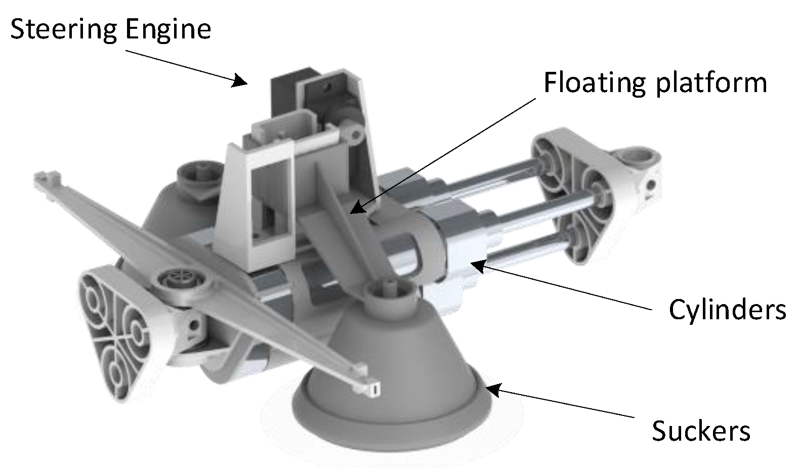
The robot’s structure is mainly composed of four segments. The structure of the first three segments of the robot is similar. As shown in Figure 1, each segment of the first three segments is arranged with cylinders along the axial direction. In order to increase the thrust of the cylinder and the rigidity of the structure, a structure in which three cylinders of the same stroke are arranged side by side is employed. The cylinder can be freely extended or shortened under the drive of the air pump, thereby changing the length of each segment and generating thrust for the movement of the robot.

There is a pair of feet in each segment of the robot. Considering the need for adsorption when the robot climbs a vertical wall, the feet adopt sealed air suction cups that can be stably adsorbed on the working surface under the driving of an air pump. The foot is mounted on a floating platform that can move along a vertical rail. Each segment of the robot is equipped with a miniature motor that changes the height of the floating platform through the slider crank mechanism. The miniature motor is independently controlled to corporate with the cylinder motion in order to prevent contact wear between the working surface and the feet. The feet are lifted up before the corresponding segment of the robot moves. After the robot becomes stationary, the feet are lowered under the control of the motor so that the feet can be adsorbed to the wall surface, the process of which is as shown in Figure 2a,b.

The main structure of the above robot skeleton is made of three-dimensional (3D) printed nylon, with high strength and rigidity. Taking into account the need for sealing, the robot’s feet are made of a denser resin and silicone rubber. For the non-load structure of the robot, such as the cover and the base for mounting electronic components, they are made of 3D printed polylactic acid (PLA).

2.2. The Design of the Steering Mechanism

As shown in Figure 3, the two adjacent segments of the robot are connected by a bearing hinge, and can rotate without resistance within a certain angle range. The left and right sides of the robot are each provided with a tendon, of which one end is fixed at the front end of Segment 1, and the other end is sequentially passed through the pulleys on the two sides of segments 2, 3 and 4, and finally wound on reels at both sides of Segment 4. The two reels are each consolidated with the output shaft of a digital servo. Since the tendon is made of nylon (0.3 mm in diameter), it can be approximated as rigidity. Therefore, by dominating the rotation angle of the digital servo, the length of the tendons can be accurately controlled, thereby realizing the controllable steering motion of the robot. For example, when the tendon on the left side is stretched and the tendon on the right side is contracted, the robot bends to the right side in the shape of a letter “C”, and vice versa.

Since the skeleton structure has three hinges, three degrees of freedom are generated. However, there only two digital servos on the left and right sides to control the structure, so the robot is in an unconstrained state. In this regard, between the first and second segments, and between the third and fourth segments, a spring is arranged on both sides of the robot, whose elastic force will assist the robot in stable motion. The specific principles of this will be detailed in Section 3. From this, we have obtained a steering mechanism based on the underactuated control principle.

2.3. The Design of the Gas Circuit and the Electric Circuit

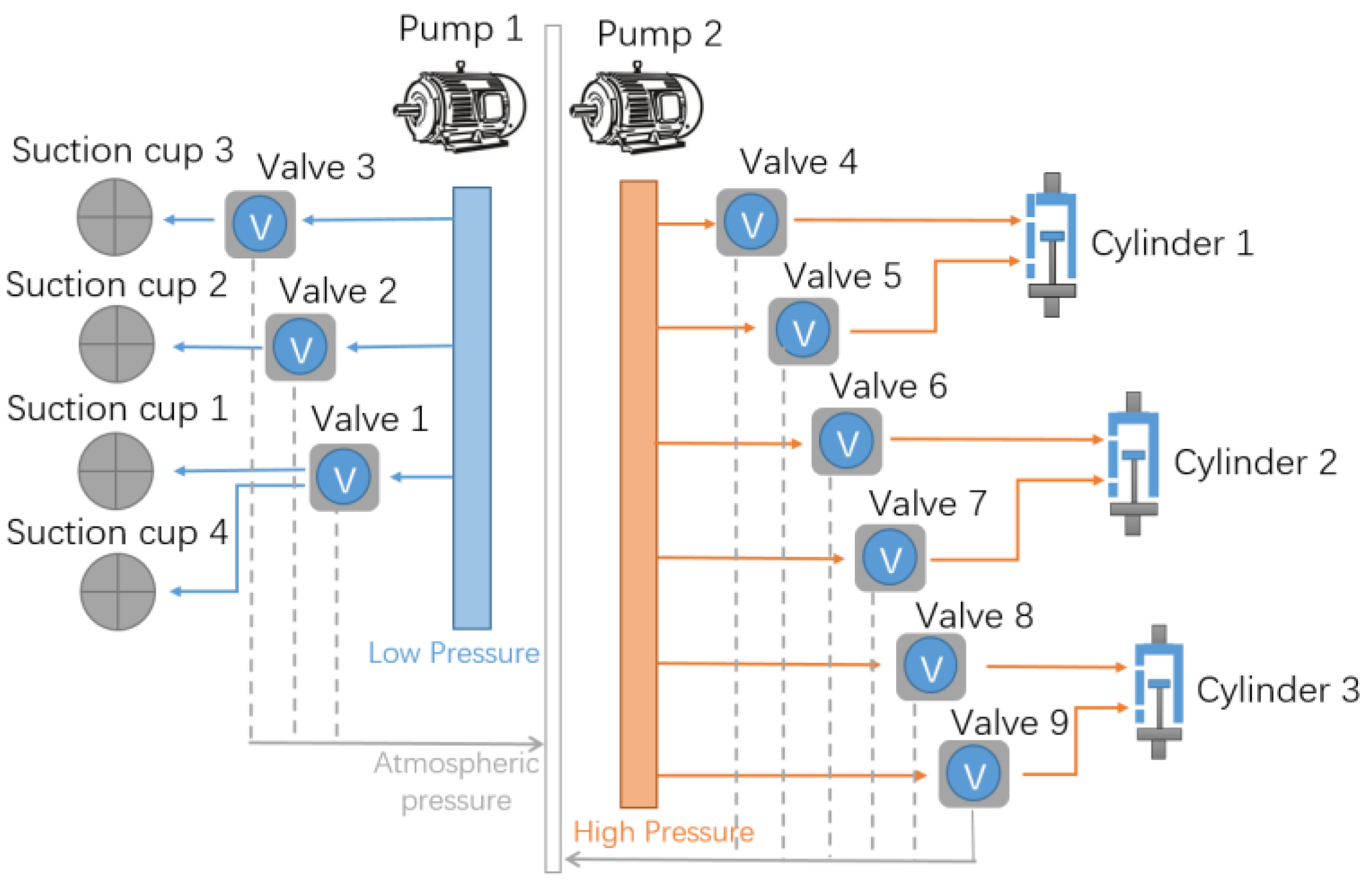
The suction cups and cylinders of the robot need to be driven by an air pump. When the robot is stationary, a single air pump can meet the requirement. However, in the process of motion, taking into account the limited gas flow rate of the air pump output, the air pressure output of the air pump may undergo a dramatic change, which is not conducive to the stable adsorption of the suction cup on the working surface. Therefore, in this particular prototype, we set up two independent gas circuits, each driven by identical but independent air pumps. As shown in Figure 4, the first air pump outputs a positive pressure for driving the telescopic movement of the cylinder, while the second air pump outputs a negative pressure for the suction cups.

We control the negative pressure in the suction cup and the positive pressure in each chamber of the cylinder through a two-position three-way electromagnetic valve, which will connect the suction cups or the chambers of cylinders with either the pump or the ambient air. Since the movements of each segment are independent from each other, it is necessary to precisely control each segment. Considering that the current in the actuators such as electromagnetic valves, air pumps, and steering gears is large and fluctuated, the voltage in the circuit might be unstable, which may affect the operation of control components such as the microcontroller unit and relays. Thus, we have set up two sets of independent circuits to power the actuator and control components, respectively.

3. Motion Process Analysis and Experiment on Horizontal Platform

3.1. Worm-Inspired Motion Process

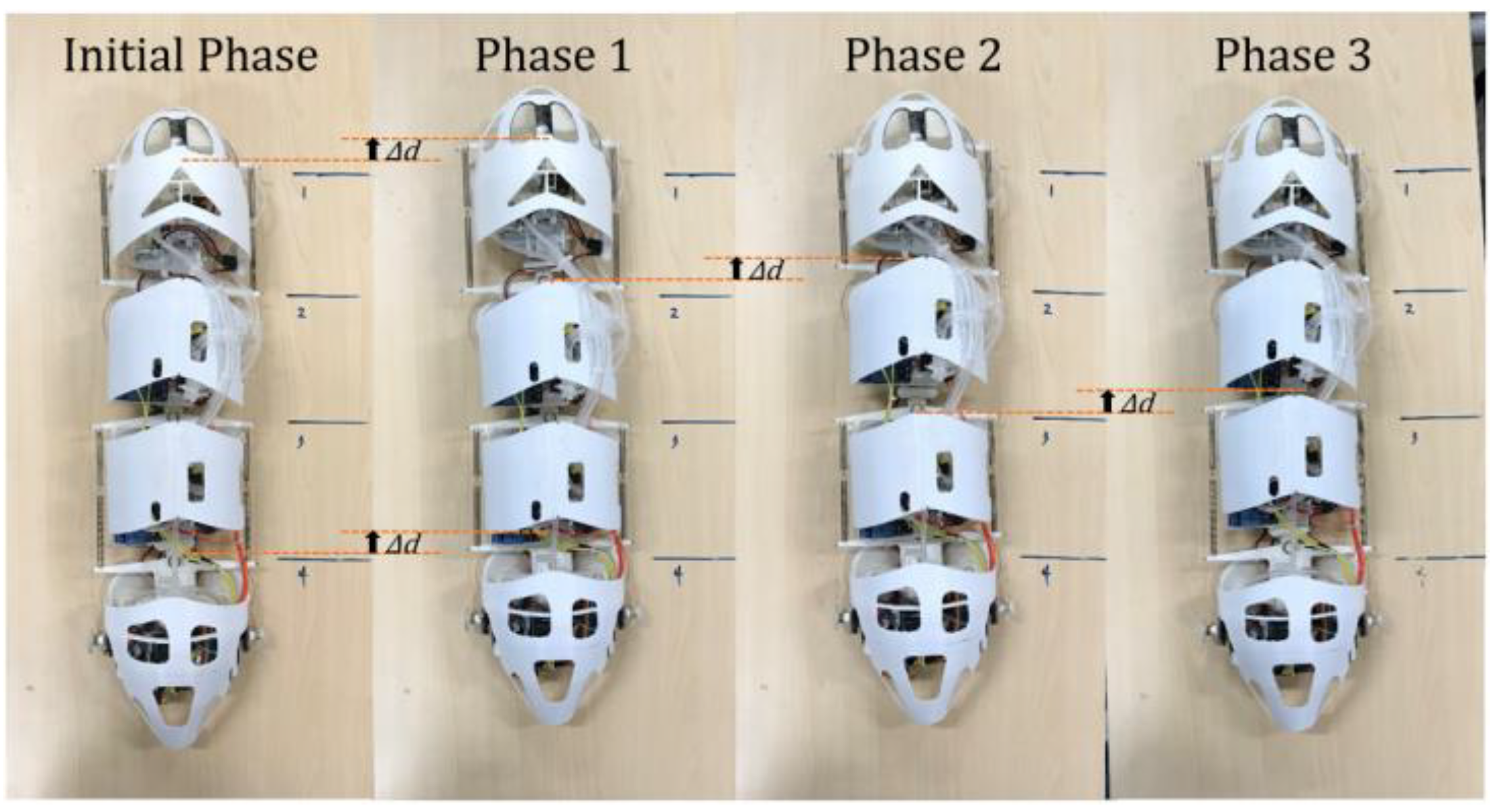
Similar to the worm movement in nature, the motion of this robot is in cycles. During each movement cycle, each segment of the worm-like robot moves forward once one by one to achieve the forward movement of the overall position. In particular, for this robot prototype, its motion cycle is divided into three phases. Assume that the state in the initial phase is as follows: cylinders in Segment 1 and Segment 2 are in the shortened state, the cylinder in the Segment 3 is in the extended state, and each foot is adsorbed on the working surface. Then, the following movements occur during the next motion cycle:

Phase 1: The feet of Segment 1 and Segment 4 are off the work surface and lifted; the remaining feet are still attached to the work surface. Then, the cylinders of Segment 1 extend and the cylinder of Segment 3 shortens; thus, Segment 1 and Segment 4 move forward until the limit stroke of the cylinder. After that, the motor drives the feet of Segment 1 and Segment 4 to be lowered, and a negative pressure is generated in the suction cups, which is then adsorbed on the working surface.

Phase 2: The feet of Segment 2 are off the work surface and lifted; the remaining feet are still attached to the work surface. Then, the cylinders of Segment 1 shorten, and the cylinder of Segment 2 extends; thus, Segment 2 moves forward until the limit stroke of the cylinder. After that, the motor drives the feet of Segment 2 to be lowered, and a negative pressure is generated in the suction cups, which is then adsorbed on the working surface.

Phase 3: The feet of Segment 3 are off the work surface and lifted; the remaining feet are still attached to the work surface. Then, the cylinders of Segment 3 extend, and the cylinder of Segment 2 shortens; thus, Segment 3 moves forward until the limit stroke of the cylinder. After that, the motor drives the feet of Segment 3 to be lowered, and a negative pressure is generated in the suction cups, which is then adsorbed on the working surface.

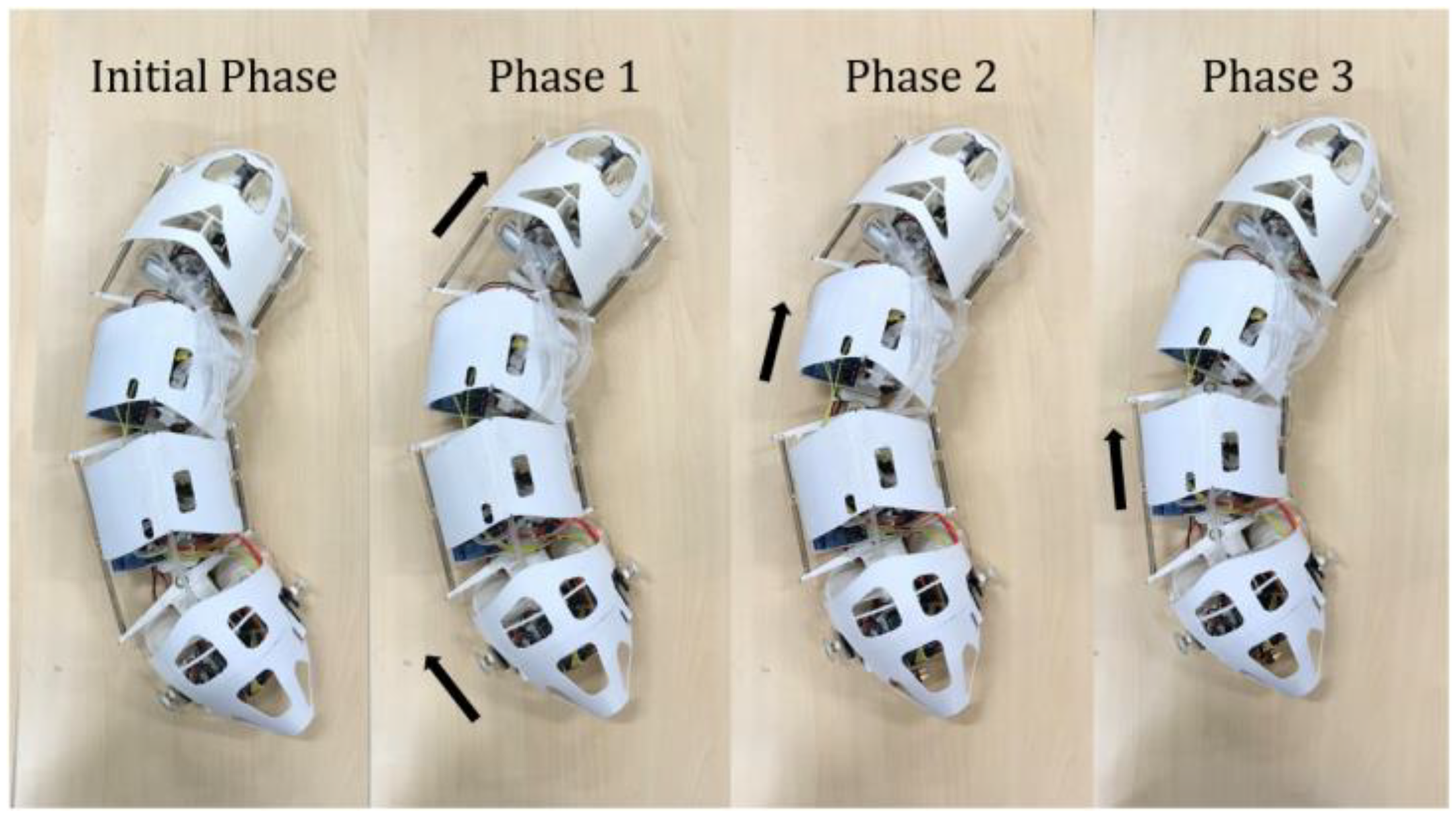
The steering motion of the worm-like robot takes place in Phase 1. When the feet of Segment 1 and Segment 4 are separated from the work surface and lifted, Segment 1 and Segment 4 are deflected to one side, centering on the hinge point by controlling the length of the tendons on the left and right sides. In subsequent movements, the robot will achieve a steering creep movement in one direction. The specific parameter control will be analyzed in Section 3.2.

The specific work processes of linear crawling and steering crawling are shown in Figure 5 and Figure 6, respectively. Figure 7 shows the input signal variation of the valve system shown in Figure 4 during a single motion cycle. It can be seen that in Phase 1, there are two segments in motion at the same time, which is a little different from phases 2 and 3, where there is only one segment in motion, respectively.

3.2. Crawling Process Analysis

The movement of this worm-inspired robot as it crawls in straight lines and turns is briefly described in Section 3.1 above. The straight crawling motion of the robot is very simple; thus, it will not be discussed here. However, the parameter control during the more complicated steering motion, that is, the specific influences of the tendons’ length on the robot posture and the subsequent motion process, is not analyzed in detail above. So, in this regard, this segment will discuss the above issue in detail.

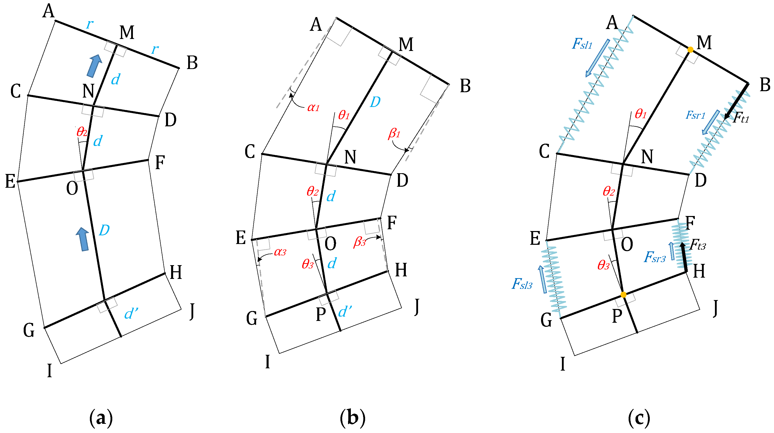
Taking the steering movement to the right as an example, as shown in Figure 8a,b, we define ${\theta }_1$, ${\theta }_2$ and ${\theta }_3$ as the deflection angles of Segment 1, Segment 2, and Segment 3 of the robot, respectively.

In Phase 1, segments 1 and 4 move forward, while segments 2 and 3 are consolidated with the ground, so the deflection angle ${\theta }_2$ is constant. At the end of Phase 1, ${\theta }_1$ and ${\theta }_3$ are mainly affected by the lengths $L_1$ and $L_2$ of the left and right tendons, so the values of ${\theta }_1$ and ${\theta }_3$ can be adjusted by changing the values of $L_1$ and $L_2$. In this way, the head and tail of this robot are deflected to one side, producing an effect similar to the worm’s steering. Assuming that width (AB) of the worm-like robot is 2r, the length of the cylinder $L_{max}=D$ and $L_{min}=d$, and the length of tendon (GI) from pulley to reel in Segment 4 is $d^{\prime }$, the geometric algorithm for the robot posture at the end of Phase 1 is solved below.

Given:

$$AM=MB=CN=NB=EO=OF=GP=PH=r$$

(1)

$$MN=NO=d$$

(2)

$$JA=BK=d^{\prime }$$

(3)

The following can be obtained from the geometric relationship:

$$BD=\sqrt{{\left(MN-MB\sin ({\theta }_1)\right)}^2+{\left(ND-MB\cos \left({\theta }_1\right)\right)}^2}$$

(4)

$$AC=\sqrt{{\left(MN+AM\sin \left({\theta }_1\right)\right)}^2+{\left(CN-AM\cos ({\theta }_1)\right)}^2}$$

(5)

$$DF=\sqrt{{\left(NO-ND\sin \left({\theta }_2\right)\right)}^2+{\left(OF-ND\cos ({\theta }_2)\right)}^2}$$

(6)

$$CE=\sqrt{{\left(NO+CN\sin \left({\theta }_2\right)\right)}^2+{\left(EO-CN\cos ({\theta }_2)\right)}^2}$$

(7)

$$FH=\sqrt{{\left(PO-OF\sin \left({\theta }_3\right)\right)}^2+{\left(PH-OF\cos ({\theta }_3)\right)}^2}$$

(8)

$$EG=\sqrt{{\left(PO+EO\sin ({\theta }_3)\right)}^2+{\left(GP-EO\cos ({\theta }_3)\right)}^2}$$

(9)

The above parameters meet:

$$L_1=JA+AC+CE+EG$$

(10)

$$L_2=KB+BD+DF+FH$$

(11)

With the simultaneous use of equations of (10) and (11), ${\theta }_1$ and ${\theta }_3$ that satisfy the condition alone can be found, thereby determining the result of the robot’s geometric posture at the end of the Phase 1. However, through building the prototype, we found in the experiment that due to the slight elastic deformation of the tendon, the actual and the theoretical values have a large deviation. Therefore, we introduced a set of springs, as shown in Figure 8c, whose original length is $x_0$, and elastic coefficient is k, and is connected between B and D, F and H, E and G, C and A, forming a new set of constraint relationships. However, in order to prevent the over-constrained phenomenon caused by the overlapping of the constraint relationship with the original geometric constraint, we put the tendon on the left in a relatively slack state (tension T is 0), thereby canceling one of the original constraints (relationship (10)).

From the perspective of force balance, since Segment 2 and Segment 3 remain stationary in Phase 1, Segment 1 can be regarded as rotating around the N-point hinge. In the figure, assuming that the deflection angle of the left spring (the angle between AC and MN) is ${\alpha }_1$, and the deflection angle of right spring (the angle between BD and the cylinder axis direction of Segment 1 (MN) is ${\beta }_1$, then the torque generated by the spring force is:

$$T_{k1}=\left(BD-x_0\right)kr\cos \left({\beta }_1\right)-\left(AC-x_0\right)kr\cos \left({\alpha }_1\right)$$

(12)

Assuming that the tendon on the right side has a pulling force of $F_{t1}$ on Segment 1, the torque generated is:

$$T_{F1}=F_{t1}r\cos ({\beta }_1)$$

(13)

According to the torque balance and simultaneous use of equations of (12) and (13), we can get:

$$T_{k1}=T_{F1}$$

(14)

$$F_{t1}r\cos ({\beta }_1)=\left(BD-x_0\right)kr\cos ({\beta }_1)-\left(AC-x_0\right)kr\cos \left({\alpha }_1\right)$$

(15)

$$F_{t1}=\frac{\left(BD-x_0\right)kr\cos \left({\beta }_1\right)-\left(AC-x_0\right)kr\cos \left({\alpha }_1\right)}{r\cos ({\beta }_1)}$$

(16)

Similarly, segments 3 and 4 can be seen as rotating around the P-point hinge. Assuming that the deflection angle of the left spring (the angle between EG and the cylinder of Segment 3 (OP)) is ${\alpha }_3$, and the deflection angle of the right spring (the angle between FH and OP) is ${\beta }_3$, then the torque generated by the spring force is:

$$T_{k3}=\left(FH-x_0\right)kr\cos \left({\beta }_3+{\theta }_3\right)-\left(EG-x_0\right)kr\cos \left({\theta }_3-{\alpha }_3\right)$$

(17)

Assuming that the tendon on the right side has a pulling force of $F_{t3}$ on Segment 4, the torque generated is:

$$T_{F3}=F_{t3}r\cos \left({\beta }_3+{\theta }_3\right)$$

(18)

According to the torque balance and simultaneous use of Equations (17) and (18), we can get:

$$T_{k3}=T_{F3}$$

(19)

$$F_{t3}r\cos \left({\beta }_3+{\theta }_3\right)=\left(FH-x_0\right)kr\cos \left({\beta }_3+{\theta }_3\right)-\left(EG-x_0\right)kr\cos \left({\theta }_3-{\alpha }_3\right)$$

(20)

$$F_{t3}=\frac{\left(FH-x_0\right)kr\cos \left({\beta }_3+{\theta }_3\right)-\left(EG-x_0\right)kr\cos \left({\theta }_3-{\alpha }_3\right)}{r\cos \left({\beta }_3+{\theta }_3\right)}$$

(21)

The experiment found that during the movement in Phase 1, due to the large tension in the tendon, it rubs against the pulleys at the corner, and therefore, there is a large resistance. As a result, the actual pulling force of the tendon acting at point B is greater than that at the point H, imposing a greater impact on the actual ${\theta }_1$ and ${\theta }_3$. Since the deflection angle of the tendon is circular, the Euler–Eytelwein equation $T_{\mathrm{load}}=T_{\mathrm{hold}}{\mathrm{e}}^{\mu \theta }$ can be used to calculate the resistance, where $\mu$ is the friction coefficient between the tendon and the reel, and $\theta$ is the angle difference of the tendon between point B and point H.

By geometric relationship:

$$\theta ={\theta }_1+{\theta }_2+{\beta }_1-{\beta }_3$$

(22)

Then, the tension of the tendon to the two points of H and B satisfies:

$$F_{t1}=F_{t3}·e^{\mu \left({\theta }_1+{\theta }_2+{\beta }_1-{\beta }_3\right)}$$

(23)

According to the simultaneous use of Equations (16), (21), and (23), we can get the force constraint:

$$\begin{array}{c}\frac{\left(FH-x_0\right)kr\cos \left({\beta }_3+{\theta }_3\right)-\left(EG-x_0\right)kr\cos \left({\theta }_3-{\alpha }_3\right)}{r\cos \left({\beta }_3+{\theta }_3\right)}\\ =e^{-\mu \left({\theta }_1+{\theta }_2+{\beta }_1-{\beta }_3\right)}\frac{\left(BD-x_0\right)kr\cos ({\beta }_1)-\left(AC-x_0\right)kr\cos ({\alpha }_1)}{r\cos ({\beta }_1)}\end{array}$$

(24)

where ${\alpha }_1$, ${\alpha }_3$, ${\beta }_1$ and ${\beta }_3$ meet:

$${\alpha }_1=ta{n}^{-1}\frac{AM-CN\cos \left({\theta }_1\right)}{MN+CN\sin ({\theta }_1)}$$

(25)

$${\beta }_1=ta{n}^{-1}\frac{MB-ND\cos ({\theta }_1)}{MN-ND\sin ({\theta }_1)}$$

(26)

$${\alpha }_3=ta{n}^{-1}\frac{EO-GP\cos ({\theta }_3)}{OP+GP\sin \left({\theta }_3\right)}$$

(27)

$${\beta }_3={\tan }^{-1}\frac{OF-PH\cos \left({\theta }_3\right)}{OP-PH\sin ({\theta }_3)}$$

(28)

In summary, according to the simultaneous use of Equations (11) and (24), the values of ${\theta }_1$ and ${\theta }_3$ at the end of Phase 1 can be obtained. Bringing the known related parameters $D=143.8\mathrm{mm}$, $d=118.8\mathrm{mm}$, $d^{\prime }=80\mathrm{mm}$, $r=82\mathrm{mm}$, $x_0=85\mathrm{mm}$, and $k=0.3\mathrm{N}/\mathrm{mm}$, we calculated the variation of deflection angles ${\theta }_1$ and ${\theta }_3$ with different $L_2$ values when ${\theta }_2=20°$ is in the initial phase, which is also experimentally measured, and the results are shown in Figure 9a. We also calculated the variation of deflection angles ${\theta }_1$ and ${\theta }_3$ with different ${\theta }_2$ values when $L_2=400\mathrm{mm}$ in the initial phase, which is also experimentally measured, and the results are shown in Figure 9b.

As is shown in Figure 9a,b, the theoretical value of ${\theta }_1$ is smaller than ${\theta }_3$ at any condition due to the large frictional resistance along the tendons; such a difference may lower the efficiency of the steering motion. The experiment results are basically in accord with the theory. However, the difference between ${\theta }_1$ and ${\theta }_3$ shown in the experiments seems to be larger than theoretical expectation, which might be caused by the friction on the bearings and the elasticity of the pipelines.

As ${\theta }_2$ is known, and ${\theta }_1$ and ${\theta }_3$ can be solved, we can further solve the length of the left tendon $L_1$. As described above, at this time, the left tendon is in a slack state, and the internal tension is 0. In order to satisfy this requirement, the length of the left tendon must not be less than a geometric minimum $L_{1\min }$:

$$L_1\ge L_{1min}=GI+AC+CE+EG$$

(29)

In Phase 2, segments 1, 3, and 4 remain fixed, and as shown in Figure 10a, point C, D, and N on Segment 2 advance to the positions of the C′, D′, and N′, respectively. At this time, the length of MN′ (the cylinder length of Segment 1) is d, the length of NN′ is D-d, and the deflection angle of Segment 1 becomes ${{\theta }_1}^{\prime }$. From the geometric relationship, we can get:

$${ON}^{\prime }=\sqrt{O{N}^2+{NN}^{\prime 2}+2ON·{NN}^{\prime }·\cos \left({\theta }_1\right)}$$

(30)

$$\frac{ON}{\sin ({{\theta }_1}^{\prime })}=\frac{{ON}^{\prime }}{\sin \left({\theta }_1\right)}=\frac{{NN}^{\prime }}{\sin \left(\phi \right)}$$

(31)

According to the simultaneous use of Equations (29) and (30), the following is obtained:

$${\theta }_1^{\prime }={\sin }^{-1}\left(\frac{ON·\sin \left({\theta }_1\right)}{\sqrt{O{N}^2+{NN}^{\prime 2}+2ON·{NN}^{\prime }·\cos \left({\theta }_1\right)}}\right)$$

(32)

$$\phi ={\sin }^{-1}\left(\frac{{NN}^{\prime }·\sin \left({\theta }_1\right)}{\sqrt{O{N}^2+{NN}^{\prime 2}+2ON·{NN}^{\prime }·\cos \left({\theta }_1\right)}}\right)$$

(33)

In Phase 3, segments 1, 2, and 4 remain fixed, and as shown in Figure 10b, points E, F, and O on Segment 3 advance to the positions of the E′, F′, and O′, respectively. At this time, the length of O′N′ is d, and the deflection angle of Segment 2 becomes ${{\theta }_2}^{\prime }$, as shown in Figure 10b. From the geometric relationship, we can get:

$$O{O}^{\prime }={ON}^{\prime }-d$$

(34)

$${PO}^{\prime }=\sqrt{P{O}^2+{OO}^{\prime 2}+2PO·{OO}^{\prime }·\cos \left({\theta }_2+\phi \right)}$$

(35)

$$\frac{PO}{\sin \left({{\theta }_2}^{\prime }\right)}=\frac{{PO}^{\prime }}{\sin \left({\theta }_2+\phi \right)}$$

(36)

According to simultaneous use of Equations (35) and (34), the value of ${{\theta }_2}^{\prime }$ at the end of Phase 3 is obtained:

$${\theta }_2^{\prime }={\sin }^{-1}\left(\frac{PO·\sin \left({\theta }_2+\phi \right)}{\sqrt{P{O}^2+{OO}^{\prime 2}+2PO·{OO}^{\prime }·\cos \left({\theta }_2+\phi \right)}}\right)$$

(37)

At this point, a motion cycle ends, and the robot returns to the state at the beginning of step 1. Based on the above Equations (11), (24), and (37), the values of ${\theta }_1$, ${\theta }_2$, and ${\theta }_3$ after any of the periodic motions can be solved. The relationship between the three values and the number of cycles T is shown in Figure 11a. It can be seen that regardless of the initial state, after several cycles of the motion, ${\theta }_1$, ${\theta }_2$, and ${\theta }_3$ will tend to a fixed value.

In addition, at the end of a motion cycle, the cylinder axis direction of Segment 2 (ON) will have a steering angle $\phi$ with respect to its original position, and we define $\phi$ as the steering angle of the robot. After a plurality of cycles, the cumulative value of the angle is defined as the cumulative steering angle ∑$\phi$ of the robot, which represents the direction change of the overall robot. The relationship between $\phi$ and ∑$\phi$ and the number of cycles T is shown in Figure 11b, from which it can be seen that after the start of the motion, the steering angle tends to a fixed value, and the cumulative steering angle is approximately linear with the number of cycles.

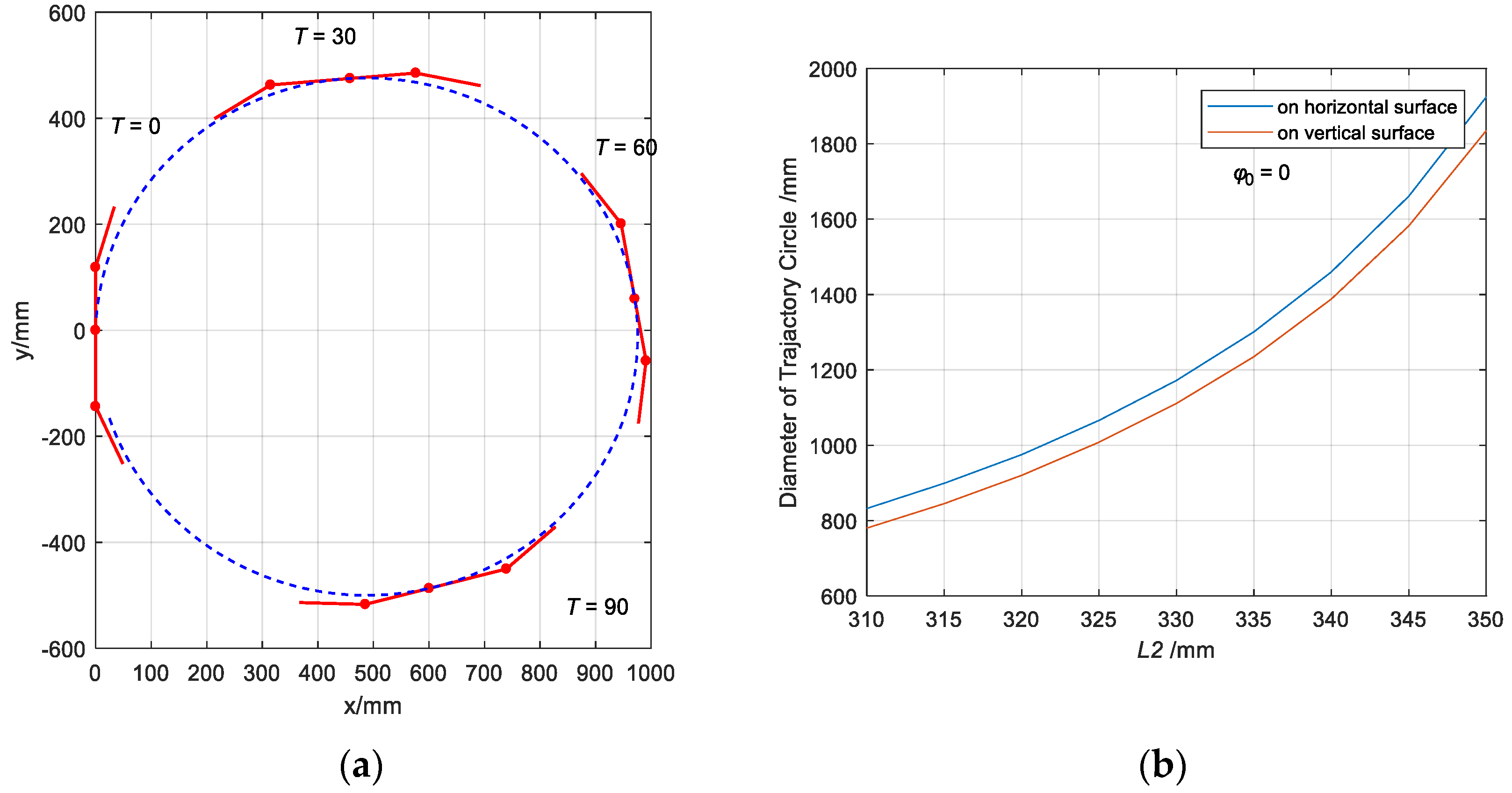
We calculate the trajectory of the robot in 120 motion cycles; the result is shown in Figure 12a. The figure shows that the motion trajectory of the robot appears to be circular if the length of the tendon remains unchanged. In a particular state, when the length of the tendon (L₂) is 400 mm, the diameter of the trajectory circle is 920 mm.

We conducted an experiment to test the steering ability of the robot. In the experiment, the robot finished a circular route and finally returned to its starting point in 128 motion cycles; the whole process took 22 minutes. The diameter of the circle is 978 mm, which is slightly bigger than the calculation results. Besides the reason of friction, which has been mentioned before, such difference might also be caused by the slippage that happened between the sucker cups and the ground.

With a scalable structure design, the robot can be added to five or more segments in practical application. In these cases, the above calculation results will be slightly different. Take an expanded robot with n segments in total for example; a single motion cycle described in Section 3.1 will consist of n−1 phases ($n\ge 3)$. During Phase 1, Segment 1 and Segment n move forward, while the others remain attached to the ground. In this process, we can still control the first and last deflection angle, ${\theta }_1$ and ${\theta }_{n-1}$ through adjusting the length of tendons, where the geometric relationship still follows the Equations (11) and (24). In any of the latter phases, only one segment moves forward, and its deflection angle and position can be solved using Equations (35) and (37). Therefore, the position and posture of the robot after a whole cycle can be precisely obtained after the motions in each phase are solved successively.

4. Climbing Performance Analysis and Experiments

4.1. Climbing Process Analysis

The robot has the ability to climb vertical walls due to the installation of pneumatic suction cups that can be attached to a vertical wall. We experimented with the climbing performance of the robot, in which the climbing process of the robot is shown in Figure 13.

However, the weight of the robot itself may affects the results in the climbing locomotion while steering sidewise. In Phase 1, the gravity of Segment 1, $M_{1}g$, and the gravity of Segment 4, $M_{4}g$ will have a torque on point N and P, as shown in Figure 14, and thus affects the value of ${\theta }_1$ and ${\theta }_3$. We define the angle between Segment 2 and the vertical direction as ${\phi }^{\prime }$, which plays an important role in Phase 1.

Similar to Equation (24), after the introduction of the torque caused by gravity, we get:

$$\begin{array}{c}\frac{\left(FH-x_0\right)kr\cos \left({\beta }_3+{\theta }_3\right)+M_{4}g·d_4\sin \left({\phi }^{\prime }-{\theta }_3\right)-\left(EG-x_0\right)kr\cos \left({\theta }_3-{\alpha }_3\right)}{r\cos \left({\beta }_3+{\theta }_3\right)}\\ =e^{-\mu \left({\theta }_1+{\theta }_2+{\beta }_1-{\beta }_3\right)}\frac{\left(BD-x_0\right)kr\cos \left({\beta }_1\right)+M_{1}g·d_1\sin \left({\phi }^{\prime }+{\theta }_1\right)-\left(AC-x_0\right)kr\cos ({\alpha }_1)}{r\cos \left({\beta }_1\right)}\end{array}$$

(38)

The angle ${\phi }^{\prime }$ in Equation (38) satisfies:

$${\phi }^{\prime }={\phi }_0+{\displaystyle \sum }\phi$$

(39)

According to Equations (11) and (38), the values of ${\theta }_1$ and ${\theta }_3$ at the end of Phase 1 can be obtained. Similar to Chapter 2, the poseur and position of the robot can be precisely calculated after a whole motion cycle. When the initial phase meets: $L_2=400\mathrm{mm}$, ${\theta }_2$ = 20°, and ${\phi }_0=0$, we calculate the trajectory of the robot during the climbing motion in 120 cycles, as shown in Figure 15a. Similar to Figure 12a, which shows the motion trajectory on a horizontal surface, this trajectory can still be considered as a circle. However, as we look closer at the figure, we find that it will take more motion cycles for the robot to return to its starting point.

We also calculate the diameter of the circle with different initial phases, as shown in Figure 15b, compared with motion on a horizontal surface, the diameter of the circle is larger during the climbing motion.

4.2. Thrust Force and Load Capacity

In order to withstand its own weight or even extra load during the climbing process, the worm-like robot needs a large traction force. As mentioned earlier, the traction force is primarily provided by the thrust of the cylinders mounted on each segment. However, in the process of the steering movement, the thrust directions of the respective cylinders are different, and considering the action of the spring and the tendon, the thrust that can be actually output finally is more affected by factors such as angles ${\theta }_1$, ${\theta }_2$, and ${\theta }_3$, and the position of the cylinder piston. Below, the thrust of the robot output in each stage will be calculated in detail, and the maximum load that each segment can withstand will also be calculated.

The prototype of the robot adopts CDJ2B16-25 cylinders; its performance parameters are shown in

Table 1. Cylinder performance parameters.

Inner Diameter	Total Minimal Length	Piston Stroke	Maximum Working Pressure
16 mm	75 mm	25 mm	±0.7 MPa

:

According to the experiment, the maximum air pressure generated by the air pump is 57 kPa, under which the maximum thrust/pull force generated by the cylinder of this type is 57 kPa. The maximum thrust $F_0$ that each cylinder can provide is $11.4\mathrm{N}$. Since each segment of the robot uses three cylinders arranged side by side, the thrust generated is $F=3F_0=34.2\mathrm{N}$.

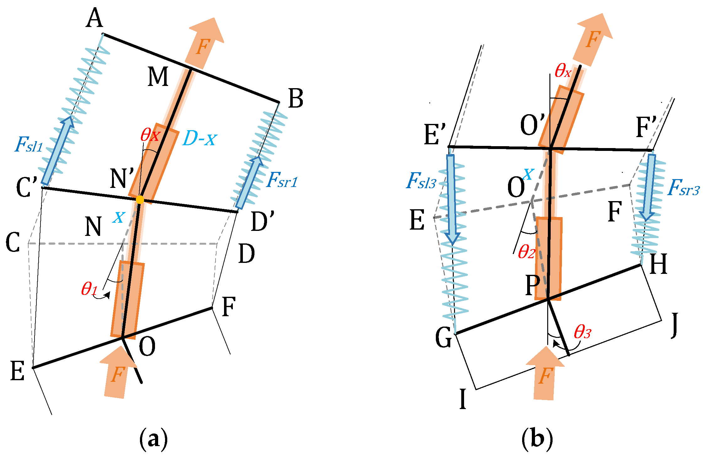
Segment 1 of the robot, during the elongation of the cylinder, is hindered by the tension of the springs on both sides and the tension of the tendon. As shown in Figure 16a, it is assumed that at a certain moment of the movement at Phase 1, the motion displacement of Segment 1 is x, the length of the first cylinder is MN $=d+x$, and the angle between Segment 1 and Segment 2 is ${\theta }_x$. Since the value of ${\theta }_x$ is small, in order to simplify the calculation, we regard AC and BD as approximately parallel. Experimental tests have shown that the above approximation has a very small adverse effect on the results. From the geometric relationship, the length of the left spring $L_{l1}\left(x\right)$ and the length of the right spring $L_{r1}\left(x\right)$ satisfy:

$$\{\begin{array}{c}{L}_{l1}\left(x\right)=r\sin ({\theta }_1)+MN\\ L_{r1}\left(x\right)=-r\sin ({\theta }_1)+MN\end{array}$$

(40)

Furthermore, the spring forces of the left spring and the right spring $F_{sl1}$ and $F_{sr1}$ meet:

$$\{\begin{array}{c}{F}_{sl1}\left(x\right)=k\left(r\sin ({\theta }_1\right)+MN-x_0)\\ F_{sr1}\left(x\right)=k\left(-r\sin ({\theta }_1\right)+MN-x_0)\end{array}$$

(41)

According to the equation of torque equilibrium centered on point N, the tension in the right tendon $F_{t1}\left(x\right)$ is obtained to satisfy:

$$F_{sl1}\left(x\right)·r=F_{sr1}\left(x\right)·r+F_{t1}·r$$

(42)

Based on simultaneous use of Equations (41) and (42), we can get:

$$F_{t1}\left(x\right)=2kr\sin ({\theta }_1)$$

(43)

The final remaining propulsion force is:

$$\begin{array}{c}{F}_1=F-F_{t1}\left(x\right)-F_{sl1}\left(x\right)-F_{sr1}\left(x\right)\\ =F-2kr\sin ({\theta }_1)-2k\left(d+x-x_0\right)\end{array}$$

(44)

It can be seen that the thrust output from Segment 1 is mainly affected by the deflection angle ${\theta }_1$ and the cylinder position $x$.

For Segment 4 of the robot, as shown in Figure 16b, the force is similar to that of Segment 1. The only difference is that the tension of the spring and the tendon is the same as the thrust of the cylinder in one direction, and the external forces will enhance the overall traction of the mechanism. In a similar way as the algorithm of Segment 1, we can get:

$$\begin{array}{c}{F}_4=F+F_{t3}\left(x\right)+F_{sl3}\left(x\right)+F_{sr3}\left(x\right)\\ =F+2kr\sin ({\theta }_3)+2k\left(D-x-x_0\right)\end{array}$$

(45)

For Segment 2 of the robot, as shown in Figure 17a, we assume that the deflection angle of Segment 1 is ${\theta }_1$ at the beginning of Phase 2. At some point in Phase 2, when the cylinder of Segment 2 has an elongation of x in the NM direction, the deflection angle of Segment 2 becomes ${\theta }_x$, as obtained by Equation (32):

$${\theta }_x={\sin }^{-1}\left(\frac{d·\sin ({\theta }_1)}{\sqrt{d^2+x^2+2dx·\cos ({\theta }_1)}}\right)$$

(46)

Since the movement of Segment 2 is affected by the simultaneous action of the front and rear cylinders, the combined thrust in the direction of motion is:

$$F_{cylinder}\left(x\right)=F\left(1+\cos ({\theta }_x)\right)$$

(47)

Since Segment 2 receives the positive tension of the spring at the same time, the following can be obtained in the same way as Equation (41):

$$\{\begin{array}{c}{F}_{sl1}\left(x\right)=k\left(r\sin ({\theta }_x\right)+{MN}^{\prime }-x_0)\\ F_{sr1}\left(x\right)=k\left(-r\sin ({\theta }_x\right)+{MN}^{\prime }-x_0)\end{array}$$

(48)

Based on the simultaneous use of Equations (47) and (48), the total traction of Segment 2 is:

$$\begin{array}{c}{F}_2=F_{cylinder}\left(x\right)+F_{sl1}\left(x\right)+F_{sr1}\left(x\right)\\ =F\left(1+\cos ({\theta }_x)\right)+k\left(D-x-x_0\right)\end{array}$$

(49)

The situation for Segment 3 is similar to that of Segment 2. The difference is that the spring force acting on Segment 3 will hinder the movement of the mechanism. From the geometric relationship, we can get:

$$\begin{array}{c}P{O}^{\prime }=\sqrt{O{O}^{\prime }{}^2+O{P}^2+2{OO}^{\prime }·OP·\cos ({\theta }_2)}\\ =\sqrt{x^2+d^2+2xd\cos ({\theta }_2)}\end{array}$$

(50)

$$\frac{OP}{\sin \left({\theta }_x\right)}=\frac{O^{\prime }P}{\sin ({\theta }_2)}$$

(51)

According to simultaneous use of Equations (50) and (51), the following is obtained:

$$\begin{array}{c}{\theta }_x={\sin }^{-1}\left(\frac{OP\sin ({\theta }_2)}{O^{\prime }P}\right)\\ ={\sin }^{-1}\left(\frac{d\sin ({\theta }_2)}{\sqrt{x^2+d^2+2xd\cos ({\theta }_2)}}\right)\end{array}$$

(52)

Similarly, since the movement of Segment 3 is affected by the simultaneous action of the front and rear cylinders, the combined thrust in the direction of motion (OO′ direction) is:

$$F_{cylinder}\left(x\right)=F\left(1+\cos ({\theta }_x)\right)$$

(53)

In the same way as Equation (41), the tension of the left spring and right spring $F_{sl3}\left(x\right)$ and $F_{sr3}\left(x\right)$ meet:

$$\{\begin{array}{c}{F}_{sl3}\left(x\right)=k\left(r\sin ({\theta }_3\right)+{PO}^{\prime }-x_0)\\ F_{sr3}\left(x\right)=k\left(-r\sin ({\theta }_3\right)+{PO}^{\prime }-x_0)\end{array}$$

(54)

According to simultaneous use of Equations (50), (53), and (54), $F_3$, the total traction of Segment 3 is:

$$\begin{array}{c}{F}_3=F_{cylinder}\left(x\right)-\left[F_{sl3}\left(x\right)+F_{sr3}\left(x\right)\right]\cos ({\theta }_x)\\ =F\left(1+\cos \left({\theta }_x\right)\right)-2k\left(\sqrt{x^2+d^2+2xd\cos ({\theta }_2)}-x_0\right)\end{array}$$

(55)

It can be seen that the thrust output in Segment 3 is mainly affected by the deflection angle of Segment 2 in the initial phase and the cylinder position $x$.

The final calculated results of each of the four segments are shown in Figure 18. If the actual conditions permit (${\theta }_1,{\theta }_2,{\theta }_3\le 25°$, $x\le 25\mathrm{mm}$), the minimum thrust of segments 1, 2, 3, and 4 are 28.59 N, 36.22 N, 66.96 N, and 62.78 N, respectively. Therefore, the maximum weight of segments 1, 2, 3, and 4 should be no more than 2.92 kg, 3.70 kg, 6.83 kg, and 6.41 kg, respectively.

5. Conclusions and Future Work

In this paper, a novel earthworm-inspired segmented crawling robot was designed, built, and tested. Its skeleton structure is made of nylon and is divided into four segments. The periodic crawling motion of the structure is actuated by pneumatic power and achieved by sequentially moving each of the segments. Compared with previous research results, this robot has the following novelties:

(1) A novel steering mechanism based on the underactuated principle is designed. By adjusting the length of tendons on both sides, the steering motion of the robot can be precisely controlled. Compared with previous worm-inspired robots with only liner motion capacity, the above steering mechanism enables our robot to have more flexible motion, similar to worms in nature. Compared with previous snake-like robots or legged robots, which use a large number of actuators to control each of the degrees of freedom independently, our robot uses only two digital servos to control the deflection angles of four segments, which makes it not only much easier to control, but also easier to fit into a miniaturization design.

(2) With suction cups mounted on the feet, the robot is able to crawl not only on horizontal planes, but also on inclined or vertical planes, which is beyond the capabilities of any of the previous earthworm-inspired robots. The floating platforms that the feet are mounted on help keep the suction cups from abrasion against the wall and make the absorption process more reliable. Moreover, as the feet of the robot adopt modular design, the suction cups can be replaced by other foot structures according to the particular environment in order to achieve better steering efficiency and speed. For example, a foot with spines can be used on porous surfaces, and magnetic feet can be used on metal surfaces.

(3) The structure of the robot is designed to be extensible, as its structure can be added to five or even more segments. Robots with different numbers of segments share the similar motion process, as discussed in Section 4.1. Such characteristics make the robot easier to be used as a general purpose modular crawling platform, because segments carrying different devices can be added to its structure in practical application.

Basing on the novelties above, we established the theoretical model of the robot during the steering process, and analyzed the theoretical relationship between the length of the tendon and the steering angle, and simulated the trajectory of the robot during the entire movement. Experiments were conducted to verify the theoretical motion characteristics. In addition, by establishing a theoretical model, we calculated the traction force that each segment of the robot can provide, and analyzed the relationship between the traction force and other parameters. We estimated the maximum load that each segment can withstand during motion.

Our robot prototype has the ability to move in two dimensions on a plane, but in further exploration, we will try to enable it to move in three dimensions, such as a pitching motion. By increasing the degree of freedom of its skeleton structure and adding a new set of tendons to control, we can enhance the robot’s working ability and obstacle avoidance in complex environments.

References

- Kim, S.; Spenko, M.; Trujillo, S.; Heyneman, B.; Mattoli, V.; Cutkosky, M.R. Whole body adhesion: Hierarchical, directional and distributed control of adhesive forces for a climbing robot. In Proceedings of the 2007 IEEE International Conference on Robotics and Automation, Roma, Italy, 10–14 April 2007; pp. 1268–1273. [Google Scholar]
- Chattunyakit, S.; Kobayashi, Y.; Emaru, T.; Ravankar, A.A. Bio-Inspired Structure and Behavior of Self-Recovery Quadruped Robot with a Limited Number of Functional Legs. Appl. Sci. 2019, 9, 799. [Google Scholar] [CrossRef]
- Yang, W.; Yang, C.; Zhang, R.; Zhang, W. A Novel Worm-inspired Wall Climbing Robot with Sucker-microspine Composite Structure. In Proceedings of the 2018 3rd International Conference on Advanced Robotics and Mechatronics (ICARM), Singapore, 18–20 July 2018; pp. 744–749. [Google Scholar]
- Armada, M.; González, P.; Jiménez, M.A.; Prieto, M. Application of CLAWAR machines. Int. J. Robot. Res. 2003, 22, 251–264. [Google Scholar] [CrossRef]
- Raven, P.H.; Johnson, G.B. Biology, 6th ed.; McGraw-Hill: New York, NY, USA, 2001; p. 1000. [Google Scholar]
- Wang, K.; Yan, G.; Ma, G.; Ye, D. An earthworm-like robotic endoscope system for human intestine: Design, analysis, and experiment. Ann. Biomed. Eng. 2009, 37, 210–221. [Google Scholar] [CrossRef] [PubMed]
- Menciassi, A.; Accoto, D.; Gorini, S.; Dario, P. Development of a biomimetic miniature robotic crawler. Auton. Robot. 2006, 21, 155–163. [Google Scholar] [CrossRef]
- Qiao, J.; Shang, J.; Goldenberg, A. Development of inchworm in-pipe robot based on self-locking mechanism. IEEE/ASME Trans. Mechatron. 2013, 18, 799–806. [Google Scholar] [CrossRef]
- Kamata, M.; Yamazaki, S.; Tanise, Y.; Yamada, Y.; Nakamura, T. Morphological change in peristaltic crawling motion of a narrow pipe inspection robot inspired by earthworm’s locomotion. Adv. Robot. 2018, 32, 386–397. [Google Scholar] [CrossRef]
- Zarrouk, D.; Sharf, I.; Shoham, M. Conditions for worm-robot locomotion in a flexible environment: Theory and experiments. IEEE Trans. Biomed. Eng. 2012, 59, 1057–1067. [Google Scholar] [CrossRef] [PubMed]
- Umedachi, T.; Shimizu, M.; Kawahara, Y. Caterpillar-Inspired Crawling Robot Using Both Compression and Bending Deformations. IEEE Robot. Autom. Lett. 2019, 4, 670–676. [Google Scholar] [CrossRef]
- Onal, C.D.; Wood, R.J.; Rus, D. An origami-inspired approach to worm robots. IEEE/ASME Trans. Mechatron. 2013, 18, 430–438. [Google Scholar] [CrossRef]
- Kamegawa, T.; Yarnasaki, T.; Igarashi, H.; Matsuno, F. Development of the snake-like rescue robot “kohga”. In Proceedings of the 2004 IEEE International Conference on Robotics and Automation (ICRA ’04), New Orleans, LA, USA, 26 April–1 May 2004; Volume 5, pp. 5081–5086. [Google Scholar]
- Daltorio, K.A.; Boxerbaum, A.S.; Horchler, A.D.; Shaw, K.M.; Chiel, H.J.; Quinn, R.D. Efficient worm-like locomotion: Slip and control of soft-bodied peristaltic robots. Bioinspir. Biomim. 2013, 8, 035003. [Google Scholar] [CrossRef] [PubMed]
- Calderón, A.A.; Ugalde, J.C.; Zagal, J.C.; Pérez-Arancibia, N.O. Design, fabrication and control of a multi-materialmulti-actuator soft robot inspired by burrowing worms. In Proceedings of the 2016 IEEE International Conference on Robotics and Biomimetics, Qingdao, China, 3–7 December 2016; pp. 31–38. [Google Scholar]
- Rafsanjani, A.; Zhang, Y.; Liu, B.; Rubinstein, S.M.; Bertoldi, K. Kirigami skins make a simple soft actuator crawl. Sci. Robot. 2018, 3, eaar7555. [Google Scholar] [CrossRef]
- Joey, Z.G.; Calderon, A.A.; Chang, L.; Perez-Arancibia, N.O. An earthworm-inspired friction-controlled soft robot capable of bidirectional locomotion. Bioinspir. Biomim. 2019, 14, 036004. [Google Scholar]
- Koh, J.S.; Cho, K.J. Omega-shaped inchworm-inspired crawling robot with large-index-and-pitch (LIP) SMA spring actuators. IEEE/ASME Trans. Mechatron. 2013, 18, 419–429. [Google Scholar] [CrossRef]
- Yuk, H.; Kim, D.; Lee, H.; Jo, S.; Shin, J.H. Shape memory alloy-based small crawling robots inspired by C. elegans. Bioinspir. Biomim. 2011, 6, 046002. [Google Scholar] [CrossRef] [PubMed]
- Kim, B.; Lee, M.G.; Lee, Y.P.; Kim, Y.; Lee, G. An earthworm-like micro robot using shape memory alloy actuator. Sens. Actuators A Phys. 2006, 125, 429–437. [Google Scholar] [CrossRef]
- Song, C.W.; Lee, S.Y. Design of a solenoid actuator with a magnetic plunger for miniaturized segment robots. Appl. Sci. 2015, 5, 595–607. [Google Scholar]
- Herath, H.; Gopura, R.; Lalitharatne, T.D. An Underactuated Linkage Finger Mechanism for Hand Prostheses. Mod. Mech. Eng. 2018, 8, 121. [Google Scholar] [CrossRef]
Figure 1.
Skeleton structure unit of the first three segments of the robot. Each unit consists of three cylinders, a pair of pneumatic suckers, and a miniature motor.
Figure 2.
The position of the feet under the control of the miniature motor: (a) the feet are lowered down when the segment is stationary; (b) the feet is lifted up before the segment’s motion starts.
Figure 3.
Top view of the overall structure of the steering mechanism. The two adjacent segment units are connected by a bearing hinge. There are two tendons on the both sides of the robot.
Figure 4.
A diagram of the air circuit that consists of two pumps, nine valves, three sets of cylinders, and four pairs of suction cups: yellow represents the positive pressure generated by the first air pump, blue represents the negative pressure generated by the second air pump, gray represents the atmospheric pressure, and the direction of the arrow is the transmission direction of the air pressure signal. This figure does not cover the up and down motion of the feet controlled by motors.
Figure 5.
Four motion phases in a single cycle of the straight crawling process.
Figure 6.
Steering crawling process in a single cycle.
Figure 7.
The solenoid valves’ control signal during the motion cycle of the robot. As shown in Figure 4, valves 1–3 control the pressure in suction cups, and valves 4–9 control the pressure in the cylinders of segments 1–3. If the solenoid valve receives high potential, the cylinder will be connected to the air pump, and if it’s low potential, the cylinder will be connected to the atmosphere.
Figure 8.
A simplified geometric model of the robot in Phase 1, where MN is the cylinder of Segment 1, NO is the cylinder of the Segment 2, and OP is the cylinder of Segment 3: (a) The state at the beginning of Phase 1; (b) The state at the end of Phase 1; (c) The simplified model after the introduction of the springs.
Figure 9.
Theoretical relationship and experimental results between the values of and and the values of and at the end of Phase 1. From the figure, we can see that is always less than , because there is a friction force on the tendon. (a) When is 20°, the relationship between the values of and and the value of ; (b) when is , the relationship between the values of and and the value of .
Figure 10.
(a) A simplified geometric model of the robot at the end of Phase 2, where ON is the cylinder of Segment 2; (b) A simplified geometric model of the robot at the end of Phase 3, where PO is the cylinder of Segment 3.
Figure 11.
The relationship between the values of , , , and at the end of Phase 1 and the number of cycles T (at the initial phase: , = 20°): (a) The curve of , , and changing with the number of cycles T; (b) the curve of steering angle and cumulative steering angle changing with the number of cycles T.
Figure 12.
(a) Simulation diagram of the motion trajectory of the robot. The blue dotted line in the figure indicates the trajectory of the robot’s center point in 120 cycles (at the initial phase: ). The red line in the figure indicates the specific position and posture of the robot when T = 0, T = 30, T = 60, and T = 90. The red dot in the figure is the three bearing hinge points of the robot. It can be seen that during the steering process, the motion trajectory of the robot is circular, and the radius is related to the initial state. (b) In a particular case, the robot can avoid an obstacle through adjusting the values of and at each of the following points: 1) A: , ; 2) B: , ; 3) C: , ; and 4) D: , .
Figure 13.
Performance demonstration of the robot climbing a vertical glass surface: (a) photos of a gait sequence on a vertical glass surface; (b) the locomotion of the robot in two minutes on a vertical glass surface; (c) the locomotion of the robot in 2 minutes on a painted wooden door.
Figure 14.
A simplified force model of the robot in Phase 1 after the introduction of gravity, where O1 is the gravity center of Segment 1, O4 is the gravity center of Segment 4, and is the angle between Segment 2 and the vertical direction.
Figure 15.
(a) Trajectory diagram of the climbing motion on a vertical surface in 120 cycles. At the initial phase (, = 20°), the trajectory can be regarded as a circle. (b) The relationship between the diameter of the circle and the length of tendon L2 in different motion patterns at the initial phase: .
Figure 16.
The force diagram at a certain point during Phase 1: (a) the force on Segment 1; (b) the force on Segment 4. In the diagram, and are the deflection angles of segments 1 and 3, and x is the cylinder elongation.
Figure 17.
(a) A brief diagram of the force in Segment 2 at a certain point during Phase 2; (b) a brief diagram of the force in Segment 3 at a certain point during Phase 3. The dotted line in the diagram is the initial position before the movement.
Figure 18.
A diagram showing the relationship between the thrust, the deflection angles of each segment, and the cylinder elongation x. Segments 2 and 3 have relatively higher thrust and thus have better load capacity, while Segment 1 and Segment 4 should be specially designed to reduce their weight.