Towards a Clinically Applicable Computational Larynx Model
by
 , ,
, ,
Hossein Sadeghi
1,* ,
,
Stefan Kniesburges
1,
Sebastian Falk
1,
Manfred Kaltenbacher
2,
Anne Schützenberger
1 and
Michael Döllinger
1 
1
Division of Phoniatrics and Pediatric Audiology at the Department of Otorhinolaryngology, Head and Neck Surgery, University Hospital Erlangen, Medical School at Friedrich-Alexander University Erlangen-Nürnberg, 91054 Erlangen, Germany
2
Institute of Mechanics and Mechatronics, Vienna University of Technology (TU Wien), 1040 Vienna, Austria
*
Author to whom correspondence should be addressed.
Appl. Sci. 2019, 9(11), 2288; https://0-doi-org.brum.beds.ac.uk/10.3390/app9112288
Submission received: 5 April 2019
/
Revised: 22 May 2019
/
Accepted: 30 May 2019
/
Published: 3 June 2019
(This article belongs to the Special Issue Computational Methods and Engineering Solutions to Voice)
Abstract
:Featured Application
Potential application in medical diagnostic and therapeutic processes in the field of voice disorders.
Abstract
The enormous computational power and time required for simulating the complex phonation process preclude the effective clinical use of computational larynx models. The aim of this study was to evaluate the potential of a numerical larynx model, considering the computational time and resources required. Using Large Eddy Simulations (LES) in a 3D numerical larynx model with prescribed motion of vocal folds, the complicated fluid-structure interaction problem in phonation was reduced to a pure flow simulation with moving boundaries. The simulated laryngeal flow field is in good agreement with the experimental results obtained from authors’ synthetic larynx model. By systematically decreasing the spatial and temporal resolutions of the numerical model and optimizing the computational resources of the simulations, the elapsed simulation time was reduced by 90% to less than 70 h for 10 oscillation cycles of the vocal folds. The proposed computational larynx model with reduced mesh resolution is still able to capture the essential laryngeal flow characteristics and produce results with sufficiently good accuracy in a significant shorter time-to-solution. The reduction in computational time achieved is a promising step towards the clinical application of these computational larynx models in the near future.
1. Introduction
Voice production is the basic and most important communication tool for humans. The ability of a person to produce normal voice or, more specifically, voiced speech depends on different factors and may change during the lifetime. These factors include predisposition, gender, training, age and state of health [1,2]. Voice disorders restrict or even inhibit the oral communication of patients. As a result, both personal and economic restrictions arise that can lead to isolation and depression in patients [3,4,5]. Furthermore, the productivity reduction of the work-related disabilities of these people can be a significant social constraint [6,7]. In this context, Ruben [8] estimated the loss to the US Gross National Product to be up to $186 billion per year assuming that only 5 to 10% of the US population suffer from communication disorders. This trend was also predicted to increase due to the change to a communication-based economy in the present century. The associated annual healthcare cost of these patients totals hundreds of million dollars, which is comparable to that for other chronic diseases [9]. In general, the negative impact of voice disorders on quality of life targets not only the occupational group but also the general population of all societies [10,11,12,13,14].
Phonation is the process of voice production in the human larynx. Periodic oscillations of the vocal folds are induced by the airflow from the lungs and produce the basic sound of the voice. This flow-induced sound is filtered in the vocal tract, forming the typical spectral characteristics of voiced speech. The production of sound sources in the larynx is a complex process which results from the fluid-structure interaction between the airflow and the structural mechanics of the tissue of the vocal folds. A major problem in voice research and clinical diagnostics is the restricted access to the larynx during phonation, which allows only visual inspection of the vibration of the vocal folds with stroboscopy [15] or high-speed videoendoscopy [16,17]. Other measuring techniques include acoustic voice measurement and electroglottography (EGG) [18], both of which provide indirect measurements of the process in the larynx. As a consequence, synthetic [19] and ex-vivo [20] larynx models have been established in experimental voice research that provide almost unconfined access to the laryngeal flow region. As an alternative and complementary method, computational models have been developed in recent decades. With the development of advanced numerical methods and improvement of computational power, more aspects of the phonation process, from glottal flow analysis [21,22,23,24,25] to mechanical analysis of oscillations of the vocal folds [26,27,28] and acoustic analysis of voice sources [29,30,31,32], have been investigated numerically in detail. These computational models have the advantage of simulating the entire process with enormously high spatial and temporal resolution in the flow region and the structural domain of the vocal fold tissue. However, the ultimate goal of employing these computational tools in clinical work, for instance as a clinically standardized pre-surgery tool, has not yet been achieved. The main reason is the high computational costs for these highly accurate simulations.
Computational fluid dynamics (CFD) and structural mechanics have been employed in recent decades to investigate biomedical processes, especially hemodynamics [33,34,35]. These computational tools have also been applied for potential pre- and post-surgical planning of cardiovascular [36,37,38] and upper airway systems [39,40,41,42,43]. Mylavarapu et al. [42] used CFD tools to develop an effective surgical strategy for patients with obstructive airway disorders by comparing different virtual surgery techniques for treating coexisting glottic and subglottic stenosis by measuring the airway resistance and pressure distribution in airway lumen. Furthermore, these tools have been employed for post-operative assessment after glottis-widening surgery to improve breathing in patients with bilateral vocal fold paralysis (BVFP) [43] and also in post-endoscopic sinus surgery of nasal cavity airflow [40].
In the field of voice disorders, only a few studies have been focused on the use of computational tools to directly support clinical work. A major problem is the incorporation of different scales in the flow and tissue dynamics and acoustics and their interactions in the phonation process. Mittal et al. [44] employed a high-resolution model based on the immersed boundary method for a fully coupled phonation process as a pre-surgery tool to identify the optimal placement position of an implant for the medialization of the paralyzed vocal fold. Additionally, they evaluated the sound sources with a hybrid approach. Unfortunately, they did not mention the computational costs of their simulations to evaluate the potential application in clinics. Xue et al. [28,45] later employed this model to investigate phonatory disorders based on vocal fold left-right asymmetry and tension imbalance and reported that a huge computational time and power were required for each of their simulations. Smith and Thomson [27] also investigated numerically another pathology, subglottic stenosis (SGS), without providing the computational costs. In a recent study, Zhang [46] used a reduced-order model of the vocal fold dynamics based on the eigenmodes of oscillations to reduce the computational effort in order to find a real-time simulation model of voice production. However, for the flow excitation, they applied a quasi-one-dimensional model. Although they claimed that the effects of flow three-dimensionality have less importance in the phonation process, many previous studies proved the significance of these effects such as glottal jet instabilities, its axis switching and the transition to turbulence on laryngeal aerodynamics and acoustics [29,47,48,49].
In a previous study [50], we showed that pure flow simulation in the numerical larynx model is able to capture all the characteristic features of laryngeal aerodynamics if realistic oscillation patterns of vocal folds are applied as the moving boundaries on the model. Furthermore, such models with forced motion of vocal fold oscillation have been reported in the literature as powerful tools for the analysis of sound generation within the larynx [29,30,31,51] with the advantage of saving the computational time consumed by a fully coupled flow-structure interaction. In our study, it was demonstrated that the total wall time (elapsed real-time) to simulate laryngeal aerodynamics with high accuracy is in the range of weeks even when employing high-performance computing (HPC) resources. This was found to be in agreement with other studies. Therefore, CFD analysis may not yet be applicable in clinical diagnostics and treatment.
The question arises of whether the accuracy of the computational models can be reduced without losing the ability to provide the relevant information for supporting physicians’ planning and decision-making processes during the treatment of patients with voice disorders. To answer this question, we reduced systematically the spatial and temporal resolution of the model and evaluated the results considering the computational costs. By making optimal use of a high-performance parallel computer cluster, we performed Large Eddy Simulations (LES) of laryngeal aerodynamics with externally imposed vocal fold dynamics for different mesh resolutions. The validity of the simulations was further evaluated by comparing the results with experimental data obtained from a synthetic larynx model with silicone vocal folds.
2. Materials and Methods
2.1. Experimental Model and Measuring Techniques
The computational larynx model is based on the experimental model introduced by Kniesburges [52] that has been further used in several other studies [32,53,54,55]. The experimental setup consisted of a mass flow generator, the subglottal channel containing the synthetic vocal folds and finally the supraglottal channel. Both of the channels had a rectangular cross-section of and a length of 190 mm. The vocal fold geometry was based on the M5 model introduced by Scherer et al. [56] and Thomson et al. [57]. The life-size synthetic vocal fold models were produced as single-layer models consisting of silicone rubber with elastic properties of Poisson’s ratio and Young’s modulus kPa. These silicone rubber vocal folds showed flow-induced periodic oscillations at a frequency of 145 Hz. In this context, it should be noted that vocal fold oscillations in humans can easily exceed several hundreds hertz [58].
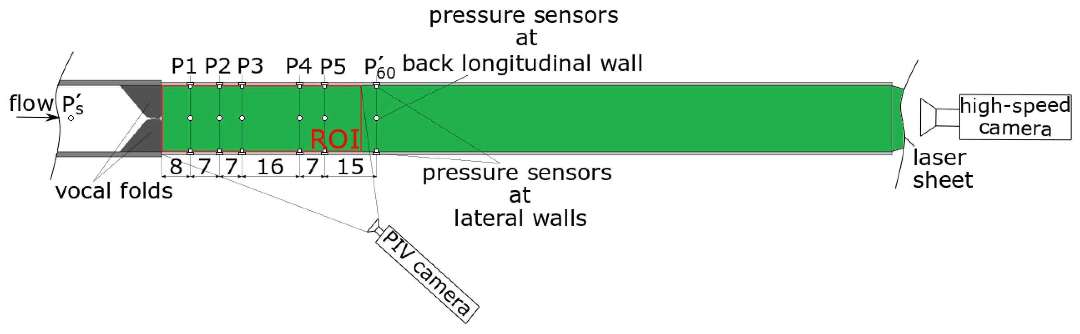
The glottal area waveform (GAW) was extracted from high-speed video footage (with a sample rate of 4000 frames per second) using the in-house software package Glottis Analyse Tool-GAT (Division for Phoniatrics and Pediatric Audiology, University Hospital Erlangen). The vocal fold models reproduced the physiological characteristics of oscillations such as periodic glottis closure and a mucosal wave-like motion with its typical convergent-to-divergent shape change of the glottal duct during an oscillation cycle [55]. Synchronously to the high-speed video visualization, the pressure distribution along the supraglottal channel was measured by pressure sensors mounted on three walls of the supraglottal channel at discrete positions, as depicted in Figure 1.
To visualize and measure the flow velocity field, a laser light sheet was guided into the supraglottal channel to illuminate the central coronal plane. The flow was seeded with water droplets and the droplet patterns were recorded with a high-speed camera. The region of interest (ROI) for the flow visualization was located immediately downstream of the vocal folds and covered 55 mm of the supraglottal channel. A phase-locked particle image velocimetry (PIV) technique was used to determine the flow velocity field at discrete instances or phase angles during an oscillation cycle. A subsequent averaging computation of the flow velocity at each phase angle yielded the phase-averaged flow field. More details about the synthetic larynx model and the experimental measuring techniques can be found elsewhere [52,53,54,55].
2.2. Numerical Model and Methods
2.2.1. Geometry of Computational Model and Vocal Fold Motion
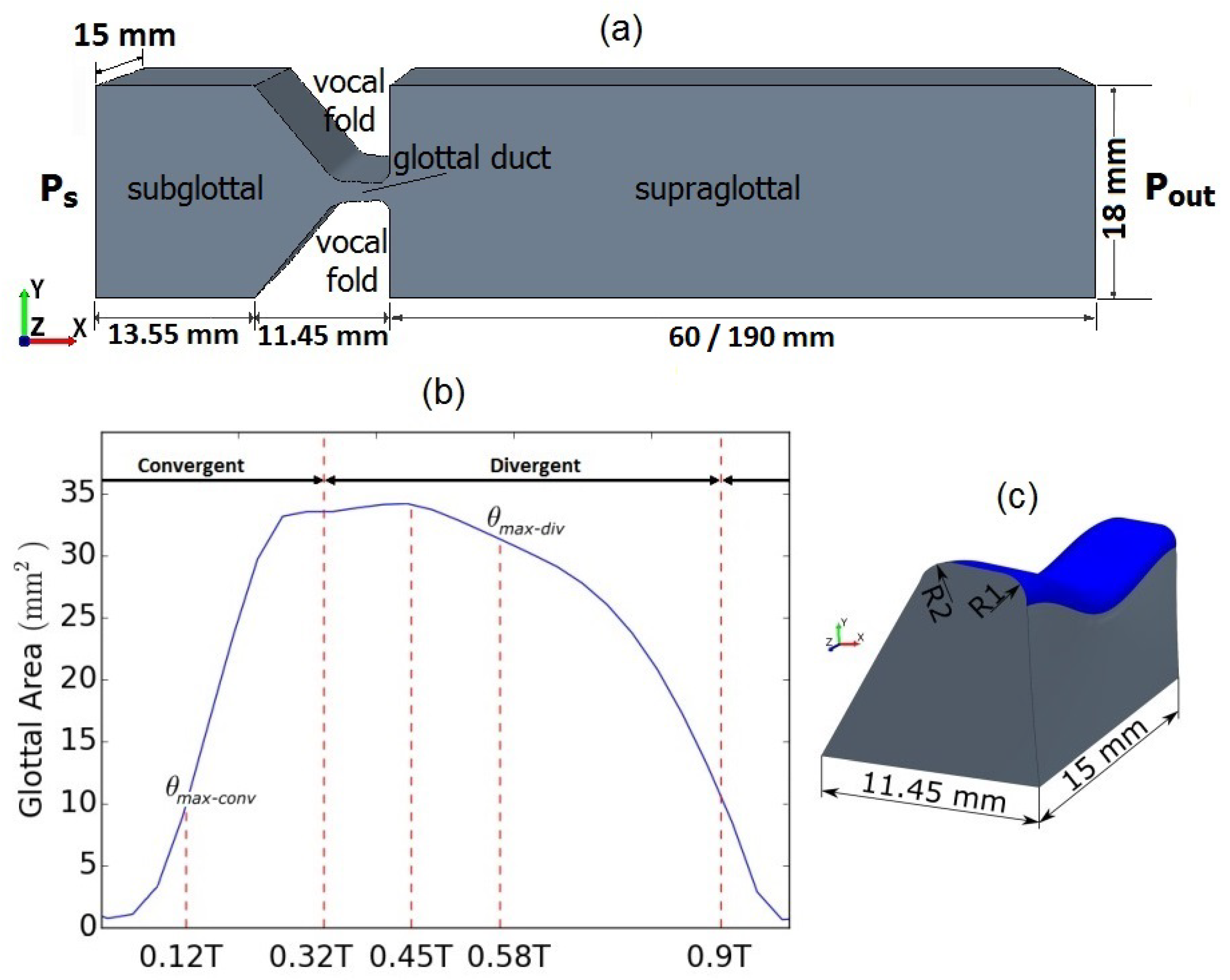
Figure 2a shows the flow domain of the computational larynx model, the shape of which is based on the experimental model shown above. The geometry of the vocal fold models and the rectangular cross-section of the sub- and supraglottal channels were kept equal to those in the experimental model. The subglottal channel of the experimental model was shortened to 25 mm in the computational model to avoid the unnecessary computational cost. The length of the supraglottal channel was also reduced to 60 mm based on the prior measurement of the glottal jet length. Another case with a longer supraglottal channel (190 mm) comparable to the experimental model was also simulated and will be introduced in Section 2.2.3.
The flow-induced oscillations of the experimental vocal fold models were reproduced in the computational model by externally forcing the motion of the vocal folds. This motion exactly reproduced the GAW (Figure 2) obtained from the high-speed visualization in the experiments. Furthermore, the same time point of the convergent-to-divergent shape change of the glottal duct and the same relationship between the vocal fold motion and the sub- and supraglottal flow devolution were maintained from the experiments.
To model the mucosal wave-like motion of the vocal folds, a translational-rotational motion was applied on the medial surface of the vocal folds (blue surface in Figure 2c), generating a maximum convergent angle and a maximum divergent angle of the glottal duct. These values were approximated from the high-speed footage of the oscillations of the silicone vocal folds and values reported in the literature [51,59,60]. The translational and rotational motions controlled the medial-lateral and the convergent-divergent motions, respectively. Finally, the translational motion was varied along the longitudinal axis of the vocal folds with a sinusoidal function to create the elliptical shape of the glottis constriction as shown in Figure 2c. More details of the modeled motion of the vocal folds can be found in Sadeghi et al. [50].
2.2.2. Numerical Methods
For the numerical model, the unsteady incompressible flow equations were solved using the software package STAR-CCM+ (Siemens PLM Software, Plano, TX, USA) with a finite-volume cell-centered non-staggered grid. LES with a WALE (wall-adapting local eddy-viscosity) [61] subgrid scale model was performed to model the turbulent flow in the larynx. A central difference scheme with second-order accuracy was used to discretize the convective and diffusive terms of the Navier-Stokes equations. These pressure-velocity linked equations were solved non-iteratively within a PISO (Pressure-Implicit with Splitting of Operators) algorithm [62]. An algebraic multigrid (AMG) method with a Gauss-Seidel relaxation scheme and biconjugate gradient accelerator was used to solve the final linear system of equations. The density and kinematic viscosity of air were considered to be and , respectively.
2.2.3. Boundary Conditions
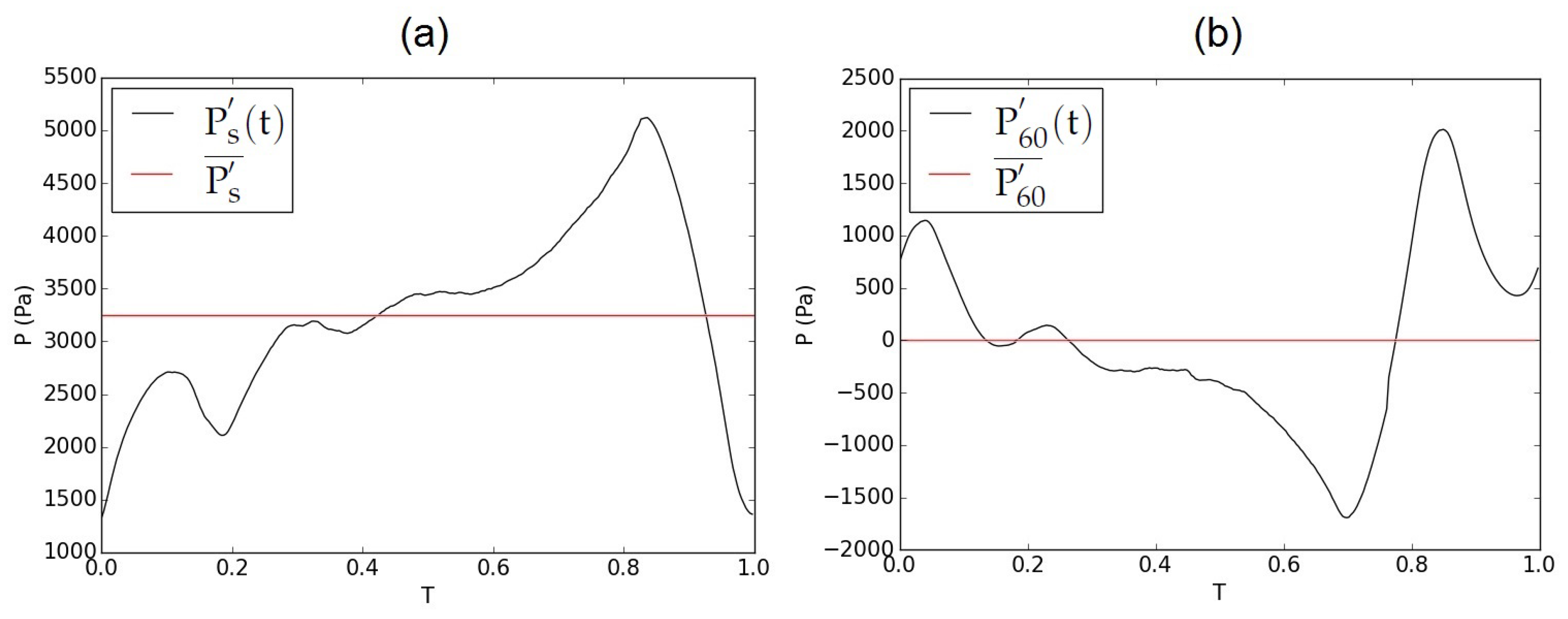
At all walls of the larynx models, no-slip no-injection boundary conditions were applied. The walls of vocal folds were defined as moving boundaries. At the inlet and outlet of the flow domain, different pressure boundary conditions were applied to identify the best combination of constant or temporal pressure evolution based on the experiments. Furthermore, two lengths of the supraglottal channel were considered as described in Section 2.2.1. In total, five simulation cases were defined as specified in Table 1. Cases C1–C4 had the shorter supraglottal channel (60 mm) and case C5 had the longer channel (190 mm) equal to the experimental model to evaluate the effect of shortening the supraglottal channel on the results. The inlet and outlet pressure boundary conditions were either pressure waveforms taken from the experiments ( and in Figure 3) or their mean values. and are the pressure waveforms measured at the subglottal channel and 60 mm downstream of the glottal exit of the synthetic larynx model, respectively. The mean values of the subglottal and supraglottal pressures were Pa and , respectively. is 0 Pa, being the relative pressure with respect to the environment. was also applied at the outlet of case C5 similar to the experimental model. Although the applied subglottal pressure is higher than the physiological values during normal phonation, such high lung pressures have been detected in special cases of phonation such as shouting, loud speech or singing [1].
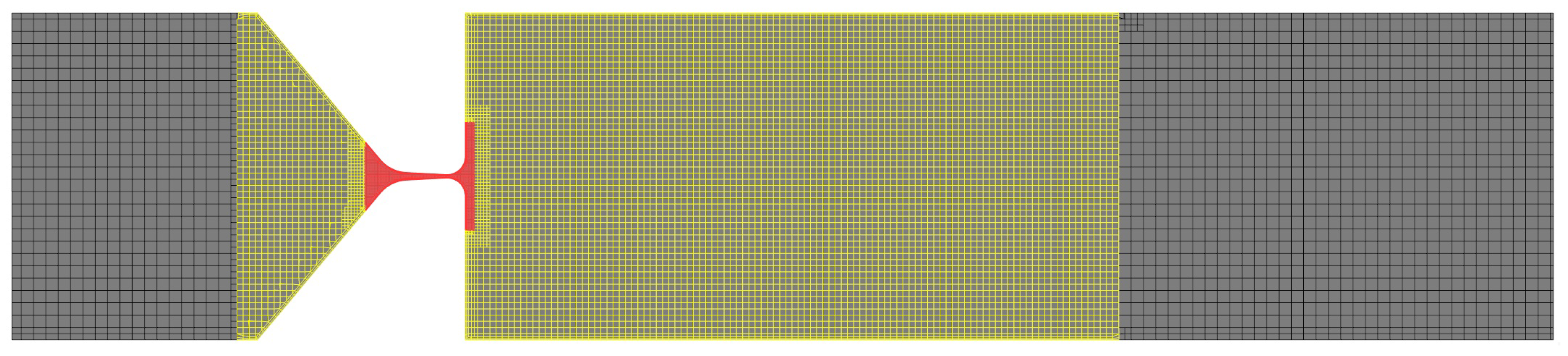
2.2.4. Mesh Generation and Mesh Motion
The starting mesh was the fine mesh proposed by Sadeghi et al. [50], which was subjected to a mesh independence study. Since the subglottal pressure in Sadeghi et al. [50] was lower than the current study, the mesh independence study was reprocessed and extended. The maximum axial velocity at the glottis and 10 mm downstream of the glottal duct exit, the mean static pressure along the center axis and the flow rate were deviated by only 0.4%, 0.01%, 1.2% and 0.07%, respectively, from the finest mesh in the mesh independence study containing approximately 40 million cells. Therefore, the proposed mesh is valid for the higher subglottal pressure applied in this study. The mesh consisted of hexahedral elements that were refined in the glottal area (glottis refinement) and near supraglottal region (Figure 4). The overset mesh approach provided by STAR-CCM+ was employed to manage the mesh motion for moving boundaries. In this method, a fixed Eulerian background mesh is assigned to the whole numerical domain and an overset mesh wrapped around each vocal fold. The cells in the overset regions are always active and deform according to the movement of the boundaries in an Arbitrary Lagrangian-Eulerian (ALE) manner. The cells in the background region are fixed and become inactive wherever they overlap with the overset cells. As a result, the total number of cells changes during an oscillation cycle depending on the distance between the vocal folds. Furthermore, some cells are required between the overset and background regions as interpolation layers. Therefore, complete closure of the glottis was not possible in this model and a minimum glottal gap of 0.2 mm was forced in the glottis during the glottal closure, which caused negligible leakage.
For this starting mesh, the total number of cells ranged between 2.1 and 2.9 million cells. The corresponding time step size was s. This led to a mean CFL number of 5 which is appropriate for implicit solvers [63,64]. More details of the mesh motion strategies and the mesh independence study can be found in Sadeghi et al. [50].
2.2.5. Reduction of Mesh Resolution
To reduce the computational costs of the numerical larynx model, the mesh resolution was reduced in this study. The aim was to answer the question of how far it is possible to decrease the mesh resolution and still obtain relevant and significant results from the numerical model. Starting with the finest and base mesh (MB), three meshes (M1–M3) were generated with systematically coarsened spatial resolution. The resulting mesh parameters and total numbers of cells are summarized in Table 2. For validation, the results obtained with the coarse meshes were compared with those obtained with the base mesh.
As mentioned by Mihaescu et al. [22], for LES modeling the mesh size should be of the order of the Taylor micro-scale (), which is a measure of the length scale of turbulence. By considering the integral length scale (a measure of the large-scale eddies) to be one order of magnitude smaller than the geometric characteristic length, which in the larynx model is the glottal width (), 10% turbulence intensity and the maximum axial velocity from the simulation with the base mesh, the Taylor micro-scale can be calculated as follows [22,65]:
The mean value of the Taylor micro-scale for the numerical simulation with the base mesh was approximately mm. Therefore, the mesh size in the glottal duct, which contains the finest mesh, was not increased above this value during the process of reduction of the mesh resolution.
Furthermore, in order to exclude the impact of the CFL number variation, the time step size was increased synchronously to the increasing mesh size with the same factor.
The requirement for some cells between the vocal folds in the closed phase of the cycle was mentioned in Section 2.2.4. The number of remaining cell layers in this area depends on the mesh size in the glottal duct. Considering this, the number of cell layers in the minimum glottal area of M3 was lower than the others, which caused deactivation of some of these cells by the overset mesh solver. As a result, the deactivated cells were replaced by wall boundary conditions and flow through them was prevented. Therefore, it was partially working like a blockage of the flow at the time of glottal closure.
3. Validation of the Computational Model
To demonstrate the validity of the computational model and find the most appropriate combination of boundary conditions, the five simulation cases shown in Table 1 were compared.
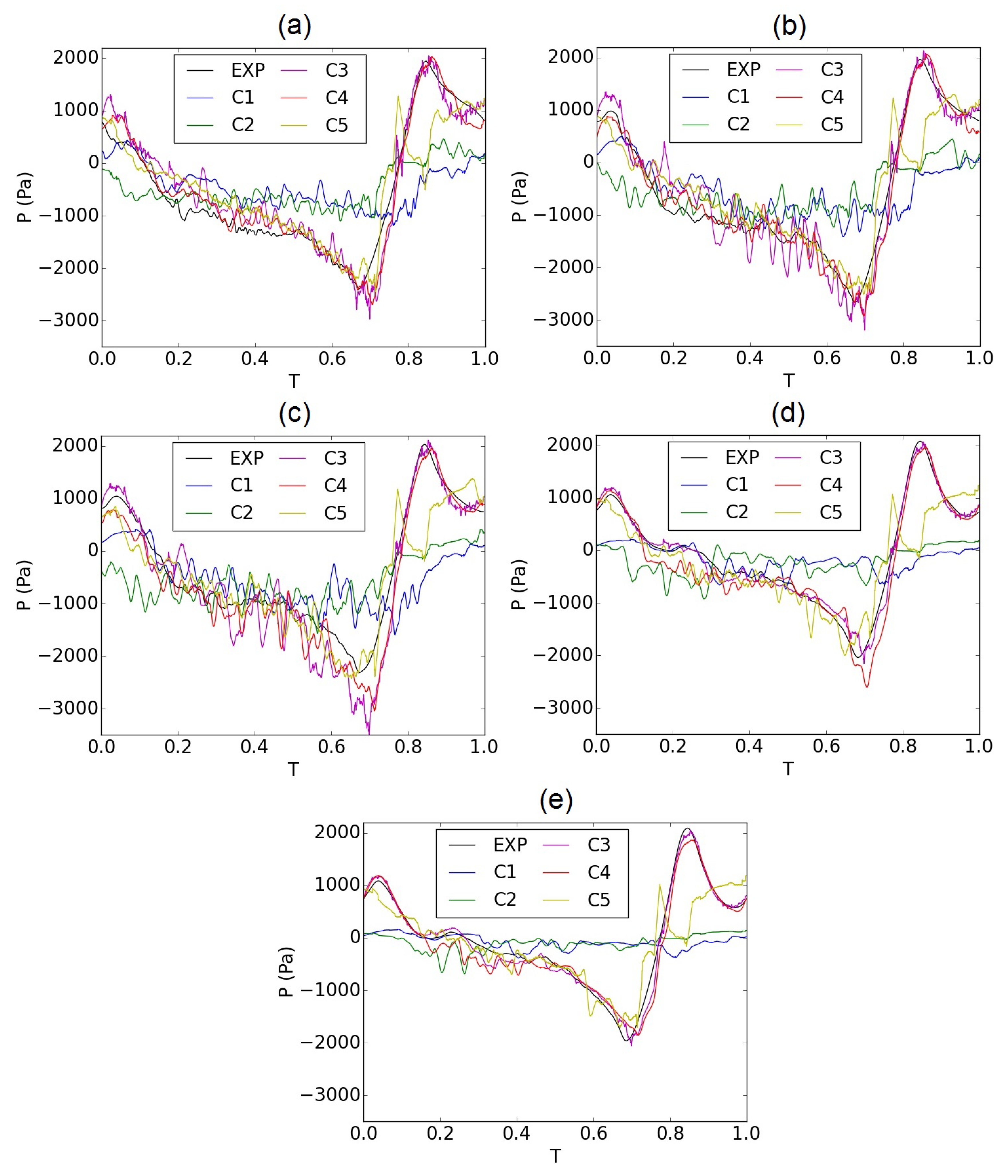
Figure 5 represents the pressure evolution at the pressure sensors in the supraglottal channel of the synthetic larynx model (P1–P5 in Figure 1) for one oscillation cycle and pressure evolutions obtained from the simulations. The three experimental pressure values at an axial position were averaged and compared with the pressure values acquired at the corresponding axial position at the center axis of the numerical model. The experimental data were best reproduced by the simulation cases C3 and C4, which have the shorter supraglottal channel, and the time-varying pressure taken from the experimental model at x = 60 mm (Figure 3b) as the outlet pressure boundary condition. In contrast to the cases C1 and C2, the choice of the time-varying outlet pressure in C3 and C4 is the key feature to produce a supraglottal flow field that is consistent with the experiments. The configuration C5 with longer supraglottal channel did indeed improve the consistency of the pressure distribution over 2/3 of the cycle, but showed deviations in the last third of the cycle, as shown in Figure 5. Furthermore, the corresponding relative error norm between the experimental and simulated pressure evolutions ( [66]) at each position provided in Table 3 revealed that C4 with the applied mean value of the experimental subglottal pressure ( Pa) at the inlet has the smallest deviation of the pressure evolution at all five axial positions. Especially in the region immediately downstream of the vocal folds, the L2 error of C4 is significantly smaller than for C3. Therefore, the most appropriate simulation case regarding the boundary conditions and length of the supraglottal channel is C4.
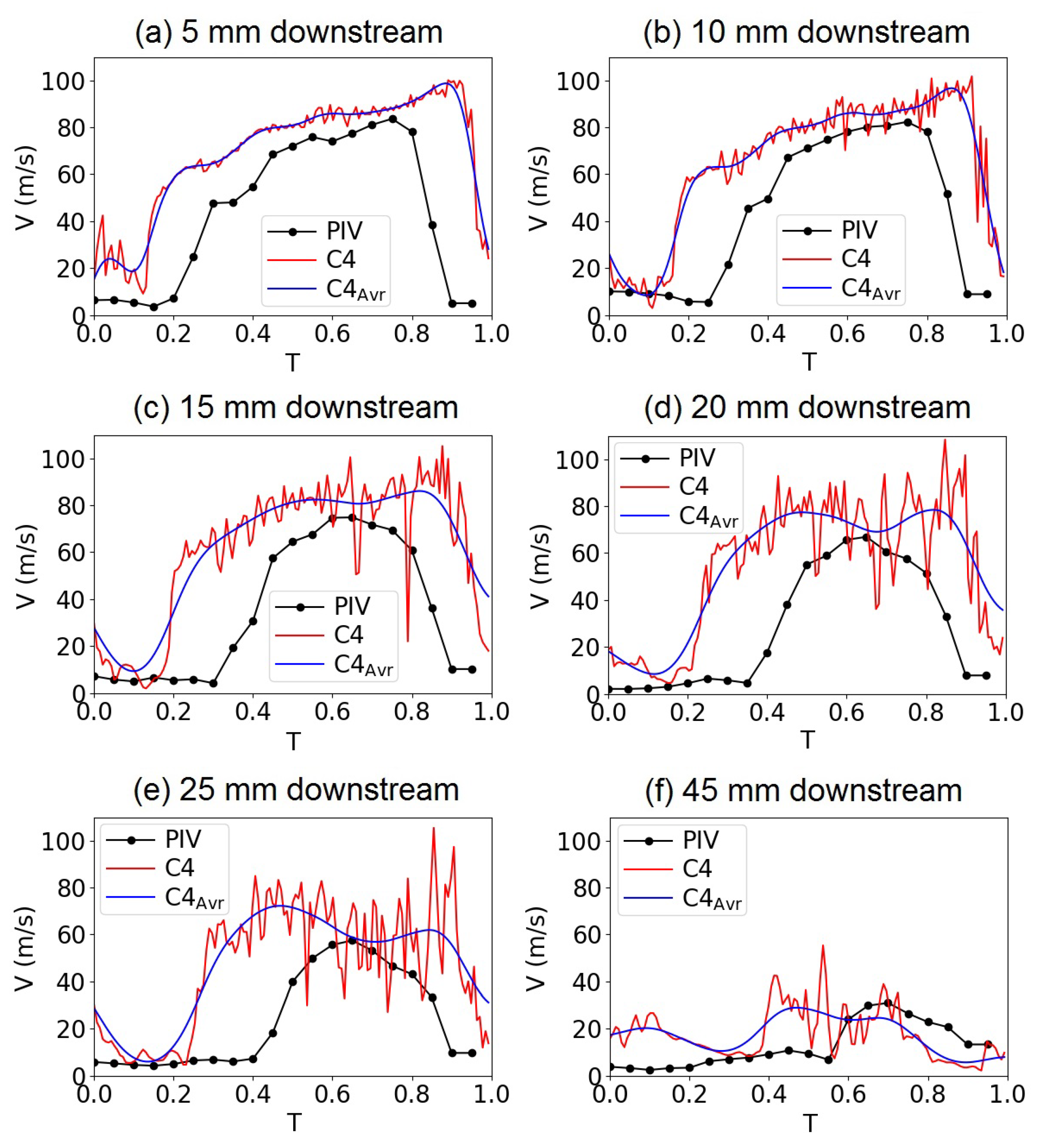
Figure 6 shows the velocity fields in the supraglottal channel in the mid-coronal plane of C4 compared with the averaged flow field obtained from the PIV measurements. Configuration C4 reproduced the typical glottal jet deflection caused by the interaction between the jet and a large recirculation area in the supraglottal channel [50,53,59,67]. Moreover, the simulated flow field shows small-scale fluctuations as shear layer instabilities that do not exist in the PIV-based flow field owing to the phase averaging. The length of the jet is also comparable between the numerical and experimental models, with slightly higher velocity values in the numerical model. This is also visible in the velocity evolution graphs in Figure 7, representing the magnitude of the velocity along the center axis of the supraglottal channel for an oscillation cycle of the computational and experimental models. The trends of the velocity evolutions are similar, especially at 5 and 10 mm downstream of the glottis exit. At larger distances, higher strength turbulent flow structures occurred in the instantaneous flow field of the numerical model. As mentioned above, those turbulent flow fluctuations are not evident in the phase-averaged flow field in the PIV measurements. The higher velocity of the jet may be due on the one hand to the phase averaging of the experimental velocities and on the other to the different subglottal pressure values between the experiment for the PIV measurement and that for supraglottal pressure measurement. The latter is the basis of the numerical model in this study. Furthermore, it seems that the jet started to develop sooner and shut off later in the cycle in the numerical case, which may be due to the different glottal area waveforms in the two experiments and also the small leakage at the beginning and end of the cycle in the numerical model.
4. Results and Discussion
4.1. Reduction of Computational Costs
The results obtained with different mesh resolutions M1–M3 (Table 2) were compared qualitatively and quantitatively with the results of the base mesh to evaluate their validity.
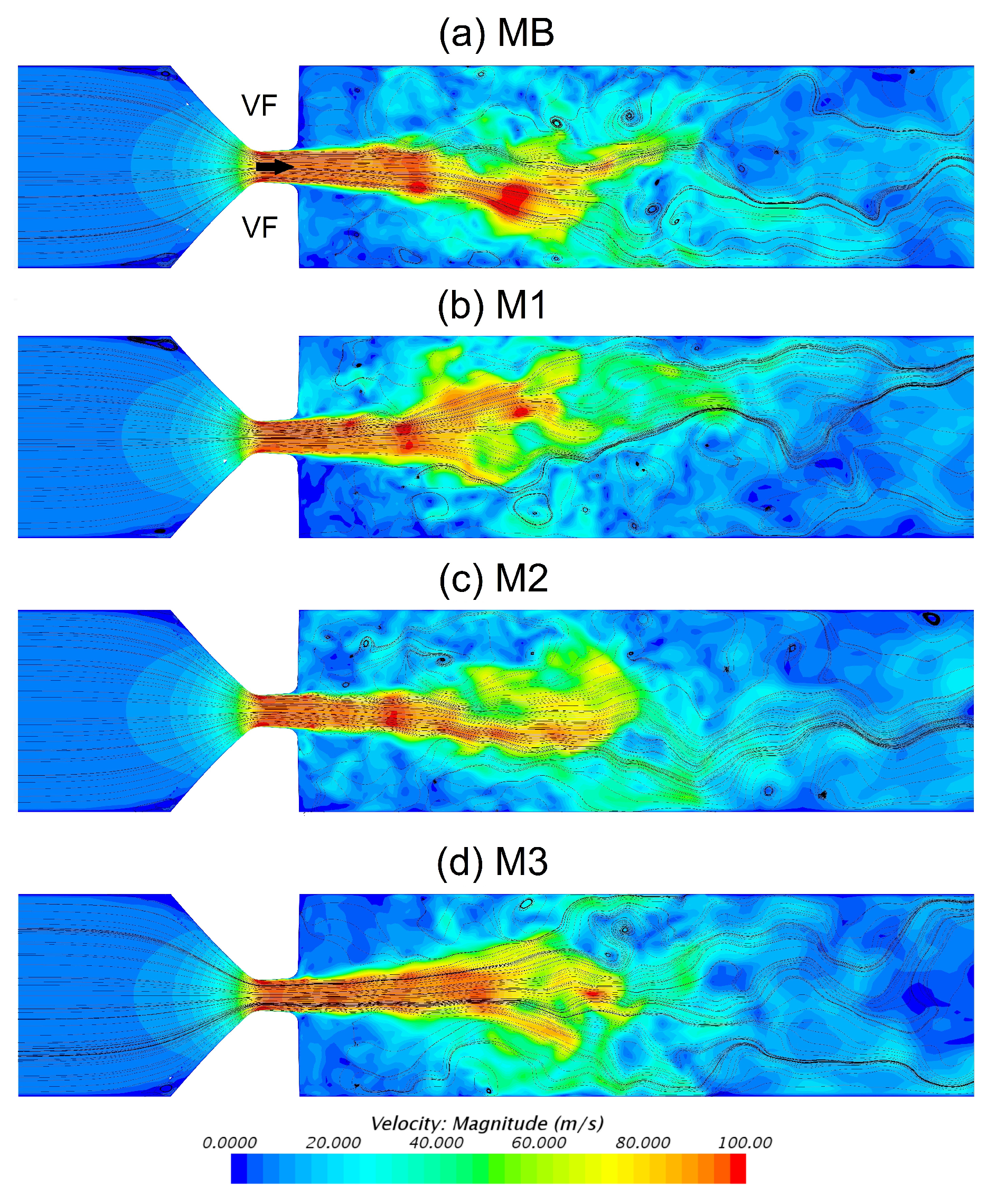
The supraglottal flow fields at a representative instance in the last quarter of the oscillation cycle are displayed in Figure 8. It can be seen that the deflection of the glottal jet, which is a characteristic feature of the laryngeal flow, was reproduced with all the mesh resolutions. In general, the jet skews either upwards or downwards depending on the flow conditions in the supraglottal channel [50,53]. In the instantaneous oscillation cycle shown in Figure 8, upward jet deflection was found for M1 and M3 and downward deflection for MB and M2.
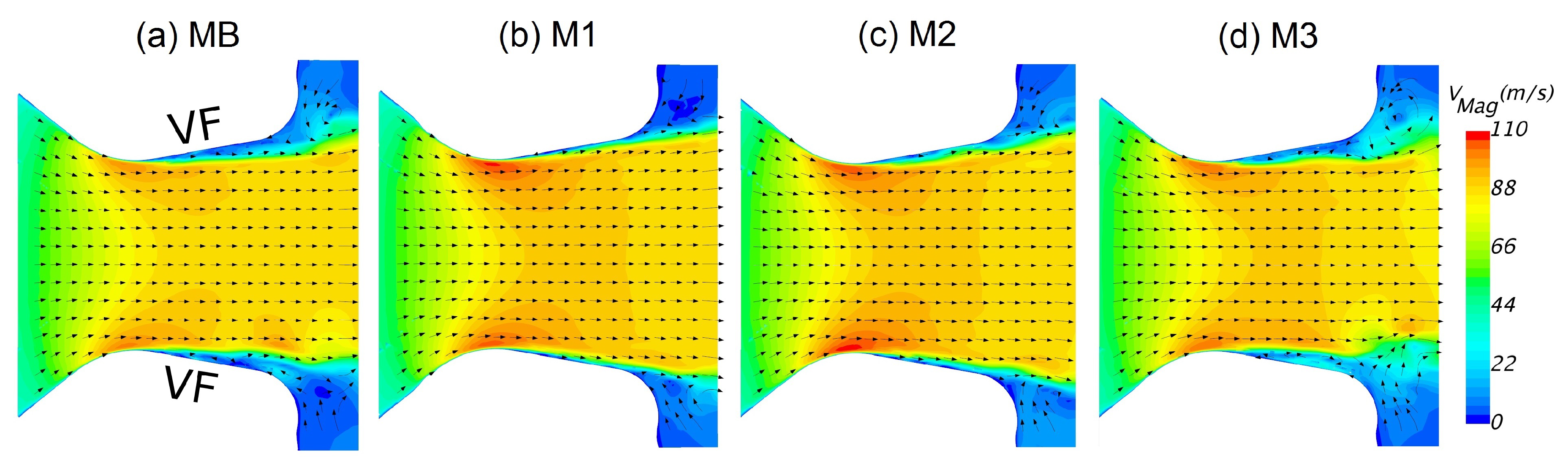
Regarding the flow field within the glottal duct (Figure 9), symmetry of the glottal jet was preserved by all the meshes. However, flow separation occurred more upstream for meshes MB and M3 whereas the jet remained attached to the glottal walls for M1 and M2. Thus, only M3 reproduced the typical intraglottal vortices in the region of separated flow. Thereby, the separation points were similarly estimated in M3 comparable to MB. These intraglottal vortices have been identified in the literature [68,69] to increase the closing forces on the vocal folds and the intensity of tonal sound.
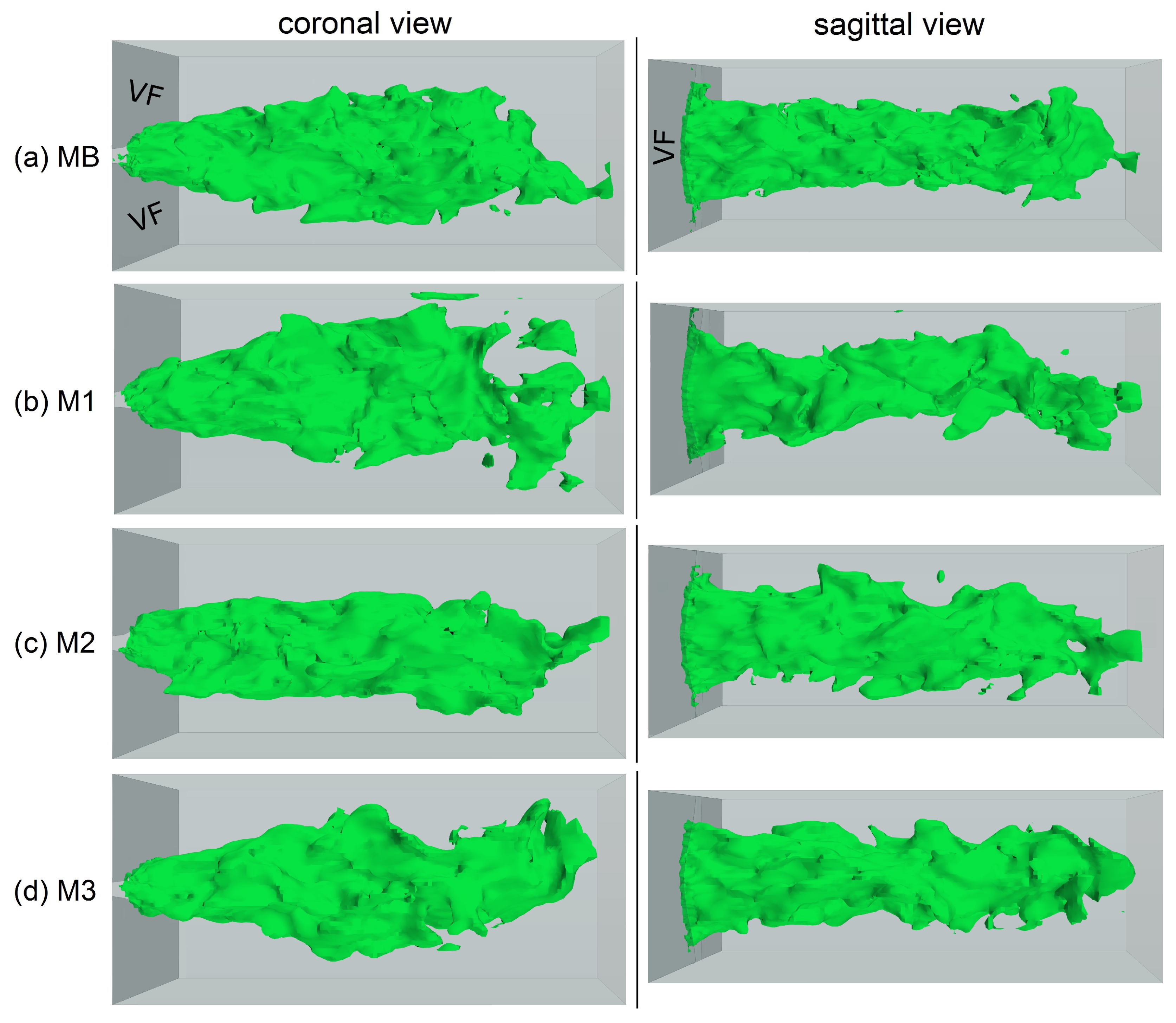
According to Hussain and Husain [70], elliptical jets show switching of the main axes in the cross-sectional plane along their streamwise evolution. This three-dimensional flow phenomenon has also been reported in experimental and numerical larynx models with elliptical glottis shapes [47,48,50,51,71]. In Figure 10, the iso-surfaces of the velocity magnitude (50 m/s) are provided at a representative time instance (0.58 T). In the coronal perspective (Figure 10, left column), the diameter of the jet increased during its streamwise evolution, whereas its diameter in the sagittal perspective (Figure 10, right column) decreased at the same time. This effect, called lengthwise vena contracta [47], was reproduced by all of the meshes. Additionally, the length of the jet was similar in all of them.
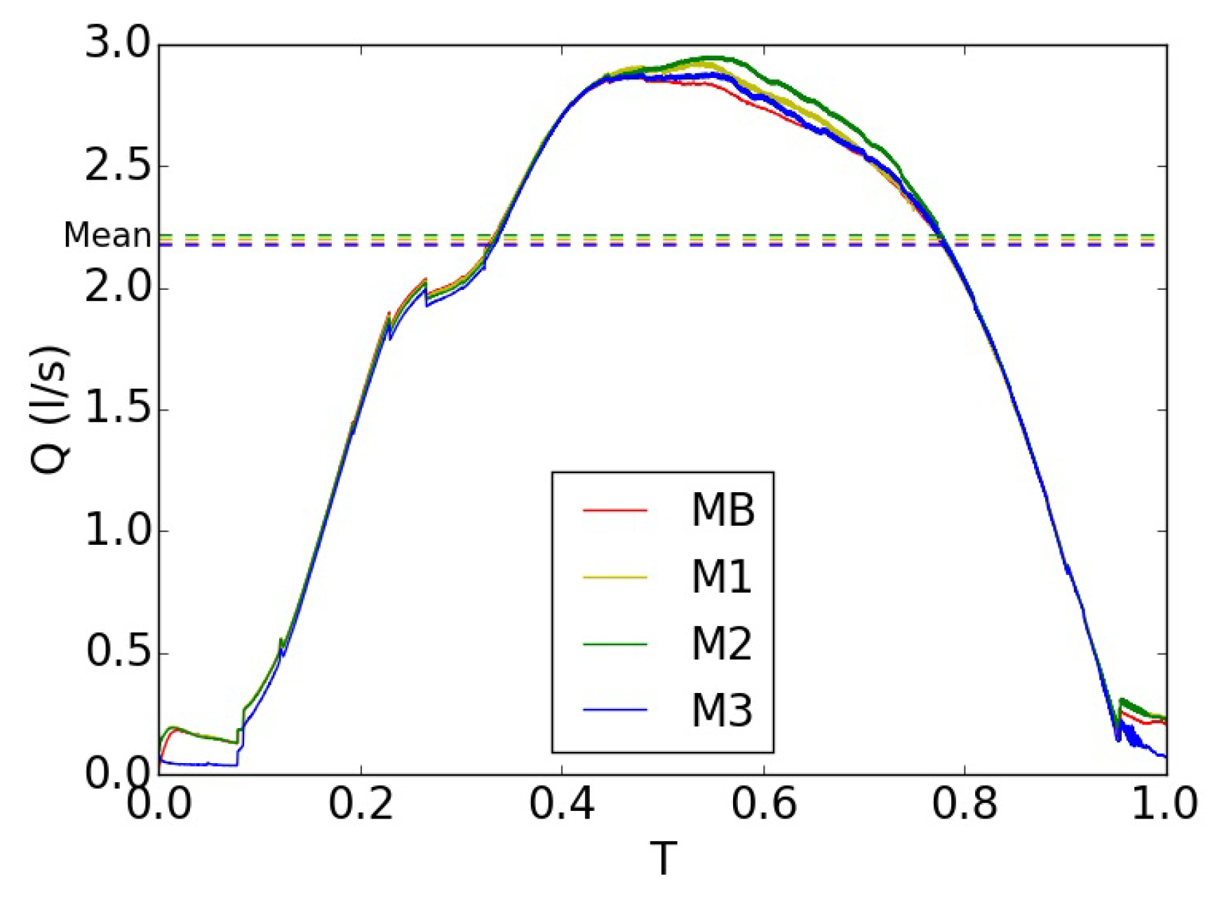
The flow rates during an oscillation cycle are shown in Figure 11 for all four mesh resolutions. Meshes M1–M3 with decreased resolutions produced a very similar trend in comparison with the base mesh MB. During the closing phase of the cycle, M1–M3 exhibited higher flow rates, with the largest deviations for M1 and M2. The reason is the full attachment of the flow to the glottal walls in these meshes for the presented cycle whereas the flow separated from the walls in M3, similar to the base mesh. Subsequently, the increase in flow rate is the result of the divergent expansion of glottal flow [72] in M1 and M2 (Figure 9b,c). The deviation of the flow rate in M3 was lowest owing to the very similar flow pattern to that of MB during the closing period.
At the very beginning and end of the cycle with the closed glottis, MB, M1 and M2 produced flow leakage, which degenerated almost to zero in M3 owing to the blockage of the glottal duct as described in Section 2.2.5.
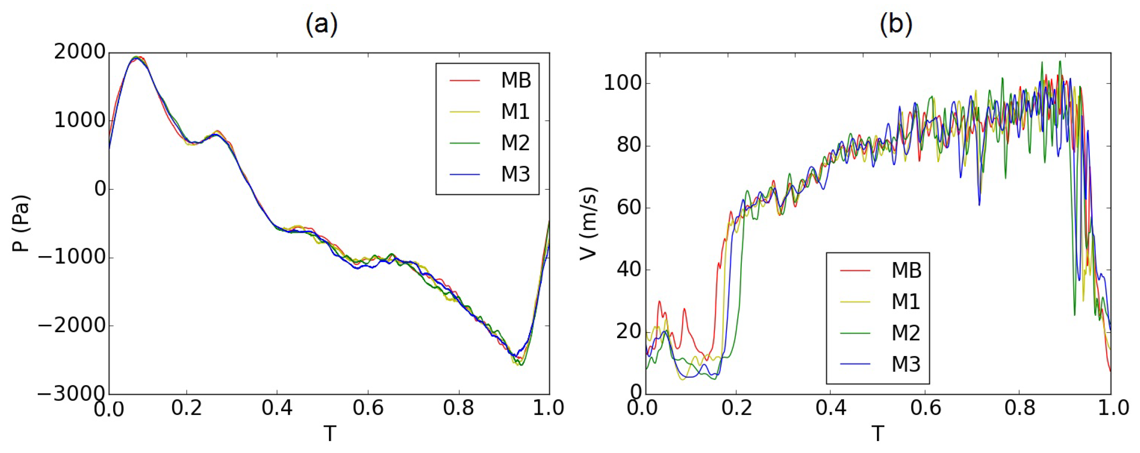
Figure 12 shows the time evolution of the instantaneous static pressure and velocity at point P1 in the near supraglottal region (Figure 1). Both graphs show good agreement of the meshes with reduced resolution (M1–M3) with the base mesh (MB) for almost the entire oscillation cycle. Only small deviations are visible in the velocity values at the beginning and end of the cycle, which are the result of different instantaneous turbulent fluctuations at point P1. Additionally, the fluctuations in the results were higher for the coarser meshes, which is obvious in the velocity evolution, especially during the closing phase of the cycle (Figure 12b). These higher fluctuations are due to the numerical noise added by the coarsening process.
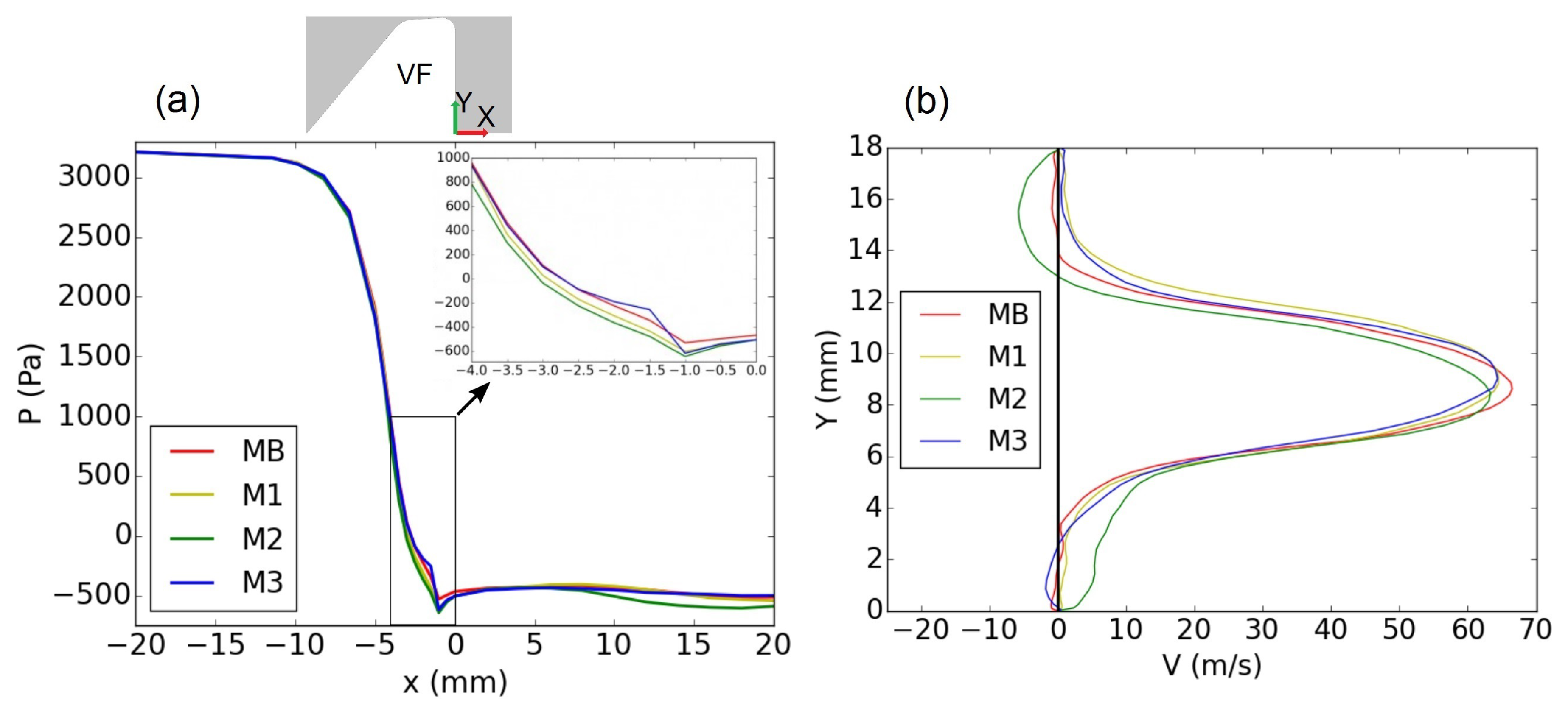
Figure 13 further shows the time-averaged pressure distribution along the center axis of the channel and the time-averaged velocity profiles in the mid-coronal plane, 8 mm downstream of the glottis exit (P1 in Figure 1). The time averaging was performed over the three simulated cycles. Again, both the mean pressure distributions and the velocity profiles of M1–M3 resembled the results obtained with MB. On evaluating the pressure values within the glottal duct and the velocity profiles in more detail, M3 showed more consistency with the base mesh MB.
Summarizing all these comparisons of flow variables, M3 with the lowest grid density among the three unexpectedly produced the best results in comparison with the base mesh MB. The L2 error norms of the presented parameters relative to the base mesh for M3 are smaller than those for M1 and M2 (Table 4). Furthermore, these errors are one order of magnitude smaller than the validation errors in Table 3. The average number of cells was reduced by more than 50% with the mesh resolution M3 compared with the base mesh. Additionally, the time step size was also increased by a factor of 1.36. As a result, the elapsed simulation time of one oscillation cycle decreased significantly to 19 h in comparison with 79 h for MB. The mentioned elapsed times are related to the parallel simulations using one compute node of the RRZE’s Emmy cluster of Erlangen-Nürnberg University, which is introduced in the next section.
4.2. Using HPC Resources to Reduce the Time-to-Solution
As already mentioned, simulation of the aerodynamics of human phonation within the larynx is computationally very expensive. To apply the computational model of the larynx in clinical routine, the use of high-performance computers is indispensable. These systems may involve single high-performance workstations with dozens of computing units up to very powerful supercomputers with hundreds or thousands of compute nodes each with tens of cores.
In this study, the RRZE’s Emmy cluster of Erlangen-Nürnberg University was employed to run the simulations. The Emmy cluster has a total of 560 compute nodes, each equipped with two Xeon 2660v2 Ivy Bridge chips (10 cores per chip + SMT) running at 2.2 GHz with 25 MB shared cache per chip and 64 GB of RAM. Hyper-Threading or SMT (Simultaneous Multithreading) permits a physical core (a single computing unit) to execute two threads (instruction sequences) simultaneously and hence appears to work like two logical cores sharing execution resources [74].
According to Amdahl’s law [75], parallel performance is restricted by the serial part of the work, the dependencies, communication between the working cores and imbalanced allocation of the threads to parallel cores, ineffective use of the shared resources, etc. Therefore, the parallel performance never increases linearly with the increase in the number of cores. Furthermore, as mentioned above, the cluster consists of multiple compute nodes, each equipped with many cores, integrated into two chips. Therefore, the scalability of the simulations in parallel execution depends on (1) the number of parallel cores in one compute node and (2) the number of nodes. In order to check the overall scalability, the simulation first ran on a single compute node with increasing number of cores. In the second step, the simulation was executed with different numbers of compute nodes, each with optimal number of cores from the first step. The parallel scalability of the simulation is shown on the basis of the elapsed simulation time (wall time) and the speed-up factor for increasing cores or nodes. The speed-up factor is the ratio of the wall time of the simulation with one core/node to the wall time with N cores/nodes.
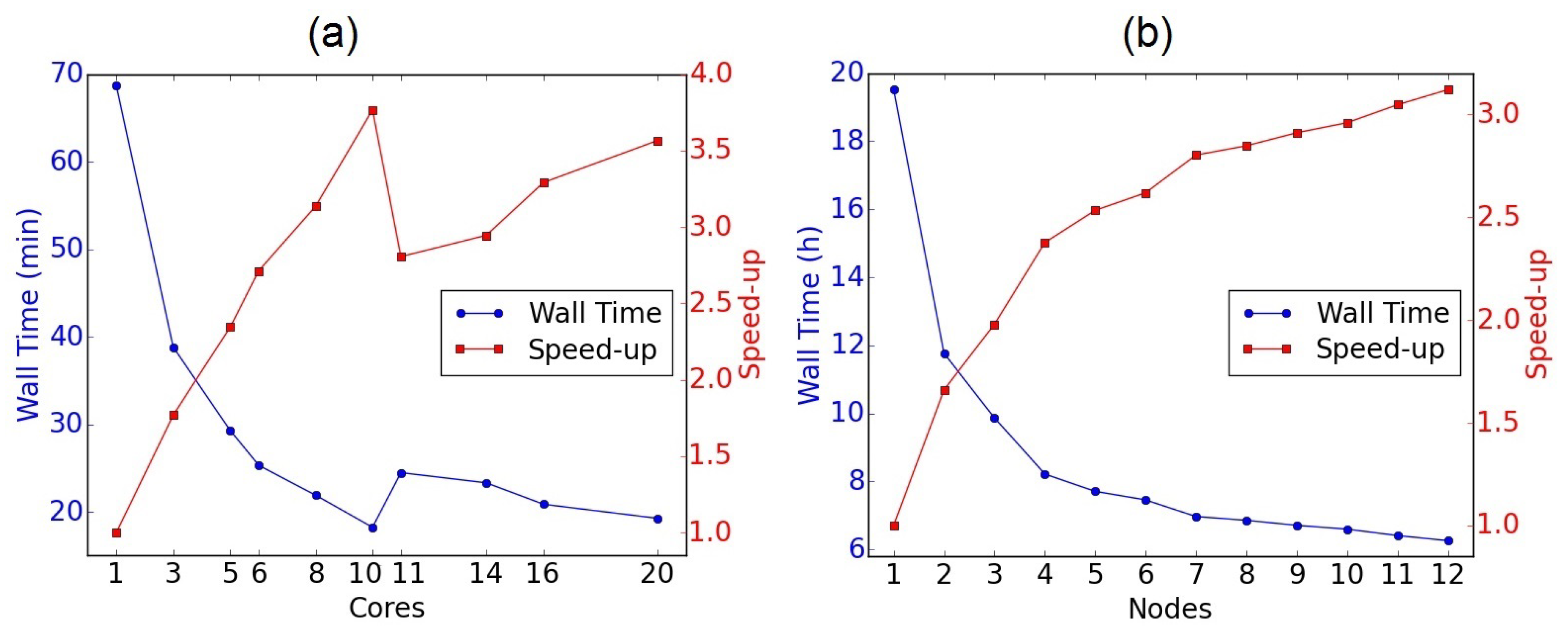
Figure 14a shows the wall time (in minutes) for a 0.1 ms simulation time and corresponding speed-up by increasing the number of physical cores within one compute node. The wall time sharply decreased for up to 10 cores, followed by a sudden increase on adding one more core. With further progress, the wall time decreased again slightly by requesting more cores. However, it never reached the minimum wall time obtained with 10 cores. The reason is that 20 threads fitted into the 10 cores of the first chip and adding more cores for computations led to the employment of the second chip. As a result, the communication time between the two chips were more than the gain on adding the extra cores which cause the drop in performance after 10 cores. Henceforth, only 10 cores of each requested compute node were employed for the following simulations.
Figure 14b demonstrates the wall time (in hours) for one oscillation cycle of the vocal folds and the corresponding speed-up as function of the requested parallel compute nodes from the cluster. It can be seen that the wall time experienced a sharp decrease on adding the second node. It decreased further on applying more compute nodes, but its gradient decreased by requesting more nodes. As result, the speed-up factor did not grow very much for a large number of compute nodes and consequently the parallel performance deteriorated. Therefore, seven compute nodes with a parallel efficiency equal to 40% of the linear scaling efficiency (based on the wall time for one node) is proposed as a good choice for running the simulations in a competitive time using reasonable resources.
To sum up, by using a total of 70 physical cores of the Emmy cluster, the simulation of 10 oscillation cycles in this numerical larynx model lasts less than 70 h.
5. Summary and Conclusions
The largest challenge in applying CFD simulations in clinical diagnostics and therapy is generating reliable results at a very short time-to-solution and with low hardware requirements. In this study, a pure CFD simulation with appropriate boundary conditions was introduced. Employing LES, the aerodynamics of the phonation process was simulated and validated with results of the experimental synthetic larynx model. The vocal fold motion was prescribed based on the oscillations of the synthetic vocal folds. The numerical model reproduced the relevant aerodynamic parameters with sufficiently good accuracy and small modeling errors. As boundary conditions, the pressure at the inlet was set to be constant, equal to the mean value of the experimental subglottal pressure, whereas the outlet pressure reproduced the temporal evolution determined in the experiments.
In the next step, the spatial and temporal resolutions of the numerical model were systematically decreased (25%, 45% and finally 55% decreases in the average number of control volumes) to reduce the computational costs. The results with these coarser meshes were compared with those obtained with the fine mesh to evaluate their validity. In general, the coarser meshes showed good agreement with the fine mesh regarding the flow pattern and aerodynamic parameters. Using the coarsest mesh, the average number of control volumes was reduced to 1.1 million cells and accordingly the time step size was increased to s. As a result, the elapsed simulation time decreased significantly by a factor of four. Finally, it was shown that the optimized use of HPC resources can reduce the wall time of simulating 10 oscillation cycles to 70 h (an approximately 75% improvement from the previous study [50] by using 30% fewer computing units), showing the potential of numerical simulations in clinical applications. However, the potential of reducing the time-to-solution is not exhausted and further improvement is required for an acceptable range of daily clinical routine. As the next steps towards a concrete clinical application, clinical MRI or CT images have to be used to generate a patient-specific geometric flow domain during phonation and the proposed model should be combined with an aeroacoustic model that may then provide new insights into the sound production and propagation process.
Author Contributions
Conceptualization, H.S., S.K., A.S. and M.D.; Formal analysis, H.S., S.K., S.F. and M.D.; Funding acquisition, S.K., M.K. and M.D.; Investigation, H.S.; Methodology, H.S.; Project administration, M.D.; Resources, S.K.; Supervision, S.K., A.S. and M.D.; Writing—original draft, H.S.; Writing—review & editing, S.K., M.K. and M.D.
Funding
This research was funded by the German Research Foundation (DFG) under DO1247/10-1 No. 391215328, the Austrian Research Council (FWF) under No. I 3702 and the Else Kröner-Fresenius Foundation (EKFS) under grant agreement No. 2016 A78.
Acknowledgments
The authors acknowledge support from the Central Institute for Scientific Computing (ZISC) and the computational resources and support provided by the Erlangen Regional Computing Center (RRZE). We acknowledge support by Deutsche Forschungsgemeinschaft and Friedrich-Alexander-Universität Erlangen-Nürnberg (FAU) within the funding program Open Access Publishing.
Conflicts of Interest
The authors declare no conflict of interest. The funders had no role in the design of the study, in the collection, analyses, or interpretation of data, in the writing of the manuscript, or in the decision to publish the results.
References
- Titze, I.R. Principles of Voice Production; National Center for Voice and Speech: Iowa City, IA, USA, 2000. [Google Scholar]
- Aronson, A.; Bless, D. Clinical Voice Disorders, 4th ed.; Thieme: New York, NY, USA, 2009. [Google Scholar]
- Smith, E.; Verdolini, K.; Gray, S.; Nichols, S.; Lemke, J.; Barkmeier, J.; Dove, H.; Hoffman, H. Effect of voice disorders on quality of life. J. Med. Speech-Lang. Pathol. 1996, 4, 223–244. [Google Scholar] [CrossRef]
- Cohen, S. Self-reported impact of dysphonia in a primary care population: An epidemiological study. Laryngoscope 2010, 120, 2022–2032. [Google Scholar] [CrossRef] [PubMed]
- Merrill, R.; Anderson, A.; Sloan, A. Quality of life indicators according to voice disorders and voice-related conditions. Laryngoscope 2011, 121, 2004–2010. [Google Scholar] [CrossRef] [PubMed]
- Roy, N.; Merrill, R.; Gray, S.; Smith, E. Voice disorders in the general population: Prevalence, risk factors, and occupational impact. Laryngoscope 2005, 115, 1988–1995. [Google Scholar] [CrossRef]
- Cohen, S.; Kim, J.; Roy, N.; Asche, C.; Courey, M. The impact of laryngeal disorders on work-related dysfunction. Laryngoscope 2012, 122, 1589–1594. [Google Scholar] [CrossRef] [PubMed]
- Ruben, R. Redefining the survival of the fittest: communication disorders in the 21st century. Laryngoscope 2000, 110, 241. [Google Scholar] [CrossRef] [PubMed]
- Cohen, S.; Kim, J.; Roy, N.; Asche, C.; Courey, M. Direct health care costs of laryngeal diseases and disorders. Laryngoscope 2012, 122, 1582–1588. [Google Scholar] [CrossRef]
- Wilson, J.; Deary, I.; Millar, A.; Mackenzie, K. The quality of life impact of dysphonia. Clin. Otolaryngol. Allied Sci. 2002, 27, 179–182. [Google Scholar] [CrossRef]
- Cohen, S.; Dupont, W.; Courey, M. Quality-of-life impact of non-neoplastic voice disorders: A meta-analysis. Ann. Otol. Rhinol. Laryngol. 2006, 115, 128–134. [Google Scholar] [CrossRef]
- Zraick, R.; Risner, B. Assessment of quality of life in persons with voice disorders. Curr. Opin. Otolaryngol. Head Neck Surg. 2008, 16, 188–193. [Google Scholar] [CrossRef]
- Slavych, B.; Engelhoven, A.; Zraick, R. Quality of life in persons with voice disorders: A review of patient-reported outcome measures. Int. J. Ther. Rehabil. 2013, 20, 308–315. [Google Scholar] [CrossRef]
- Merrill, R.; Tanner, K.; Merrill, J.; McCord, M.; Beardsley, M.; Steele, B. Voice symptoms and voice-related quality of life in college students. Ann. Otol. Rhinol. Laryngol. 2013, 122, 511–519. [Google Scholar] [CrossRef] [PubMed]
- Wendler, J. Stroboscopy. J. Voice 1992, 6, 149–154. [Google Scholar] [CrossRef]
- Döllinger, M. The next step in voice assessment: High-speed digital endoscopy and objective evaluation. Curr. Bioinf. 2009, 4, 101–111. [Google Scholar] [CrossRef]
- Döllinger, M.; Lohscheller, J.; McWhorter, A.; Kunduk, M. Variability of normal vocal fold dynamics for different vocal loading in one healthy subject investigated by phonovibrograms. J. Voice 2009, 23, 175–181. [Google Scholar] [CrossRef] [PubMed]
- Kitzing, P. Clinical applications of electroglottography. J. Voice 1990, 4, 238–249. [Google Scholar] [CrossRef]
- Murray, P.; Thomson, S. Synthetic, multi-Layer, self-Oscillating vocal fold model fabrication. J. Vis. Exp. JoVE 2011, e3498. [Google Scholar] [CrossRef]
- Luo, R.; Kong, W.; Wei, X.; Lamb, J.; Jiang, J. Development of excised larynx. J. Voice 2018. [Google Scholar] [CrossRef]
- Scherer, R.; Torkaman, S.; Afjeh, A. Intraglottal pressures in a three-dimensional model with a non-rectangular glottal shape. J. Acoust. Soc. Am. 2010, 128, 828–838. [Google Scholar] [CrossRef] [Green Version]
- Mihaescu, M.; Khosla, S.M.; Murugappan, S.; Gutmark, E. Unsteady laryngeal airflow simulations of the intra-glottal vortical structures. J. Acoust. Soc. Am. 2010, 127, 435–444. [Google Scholar] [CrossRef]
- Šidlof, P.; Horáček, J.; Řidký, V. Parallel CFD simulation of flow in a 3D model of vibrating human vocal folds. Comput. Fluids 2013, 80, 290–300. [Google Scholar] [CrossRef]
- Zörner, S.; Kaltenbacher, M.; Döllinger, M. Investigation of prescribed movement in fluid-structure interaction simulation for the human phonation process. Comput. Fluids 2013, 86, 133–140. [Google Scholar] [CrossRef] [PubMed]
- Alipour, F.; Scherer, R.C. Time-dependent pressure and flow behavior of a self-oscillating laryngeal model with ventricular folds. J. Voice 2015, 29, 649–659. [Google Scholar] [CrossRef] [PubMed]
- Duncan, C.; Zhai, G.; Scherer, R.C. Modeling coupled aerodynamics and vocal fold dynamics using immersed boundary methods. J. Acoust. Soc. Am. 2006, 120, 2859–2871. [Google Scholar] [CrossRef] [PubMed]
- Smith, S.L.; Thomson, S.L. Effect of inferior surface angle on the self-oscillation of a computational vocal fold model. J. Acoust. Soc. Am. 2012, 131, 4062–4075. [Google Scholar] [CrossRef] [PubMed]
- Xue, Q.; Mittal, R.; Zheng, X.; Bielamowicz, S.A. Computational modeling of phonatory dynamics in a tubular three-dimensional model of the human larynx. J. Acoust. Soc. Am. 2012, 132, 1602–1613. [Google Scholar] [CrossRef] [Green Version]
- Zhang, C.; Zhao, W.; Frankel, S.; Mongeau, L. Computational aeroacoustics of phonation, Part II: Effects of flow parameters and ventricular folds. J. Acoust. Soc. Am. 2002, 112, 2147–2154. [Google Scholar] [CrossRef]
- Bae, Y.; Moon, Y.J. Computation of phonation aeroacoustics by an INS/PCE splitting method. Comput. Fluids 2008, 37, 1332–1343. [Google Scholar] [CrossRef]
- Šidlof, P.; Zörner, S.; Hüppe, A. A hybrid approach to the computational aeroacoustics of human voice production. Biomech. Model. Mechanobiol. 2015, 14, 473–488. [Google Scholar] [CrossRef]
- Lodermeyer, A.; Tautz, M.; Becker, S.; Döllinger, M.; Birk, V.; Kniesburges, S. Aeroacoustic analysis of the human phonation process based on a hybrid acoustic PIV approach. Exp. Fluids 2018, 59, 13. [Google Scholar] [CrossRef]
- Jeong, W.; Rhee, K. Hemodynamics of cerebral aneurysms: Computational analyses of aneurysm progress and treatment. Comput. Math. Methods Med. 2012, 2012. [Google Scholar] [CrossRef] [PubMed]
- Radaelli, A.; Augsburger, L.; Cebral, J.; Ohta, M.; Rüfenacht, D.; Balossino, R.; Benndorf, G.; Hose, D.; Marzo, A.; Metcalfe, R.; et al. Reproducibility of haemodynamical simulations in a subject-specific stented aneurysm model—A report on the Virtual Intracranial Stenting Challenge 2007. J. Biomech. 2008, 41, 2069–2081. [Google Scholar] [CrossRef] [PubMed]
- Pereira, V.; Brina, O.; Gonzalez, A.; Narata, A.; Ouared, R.; Karl-Olof, L. Biology and hemodynamics of aneurismal vasculopathies. Eur. J. Radiol. 2013, 82, 1606–1617. [Google Scholar] [CrossRef] [PubMed]
- Brown, A.; Shi, Y.; Marzo, A.; Staicu, C.; Valverde, I.; Beerbaum, P.; Lawford, P.; Hose, D. Accuracy vs. computational time: Translating aortic simulations to the clinic. J. Biomech. 2012, 45, 516–523. [Google Scholar] [CrossRef] [PubMed]
- Morris, P.; Narracott, A.; Kobligk, H.; Soto, D.; Hsiao, S.; Lungu, A.; Evans, P.; Bressloff, N.; Lawford, P.; Hose, D.; et al. Computational fluid dynamics modelling in cardiovascular medicine. Heart 2016, 102, 18–28. [Google Scholar] [CrossRef]
- Ueda, T.; Suito, H.; Ota, H.; Takase, K. Computational fluid dynamics modeling in aortic diseases. Cardiovasc. Imaging Asia 2018, 2, 58–64. [Google Scholar] [CrossRef]
- Zachow, S.; Steinmann, A.; Hildebrandt, T.; Weber, R.; Heppt, W. CFD simulation of nasal airflow: Towards treatment planning for functional rhinosurgery. Int. J. Comput. Assist. Radiol. Surg. 2006, 165–167. [Google Scholar] [CrossRef]
- Xiong, G.; Zhan, J.; Zuo, K.; Li, J.; Rong, L.; Xu, G. Numerical flow simulation in the post-endoscopic sinus surgery nasal cavity. Med. Biol. Eng. Comput. 2008, 46, 1161–1167. [Google Scholar] [CrossRef]
- Chen, X.; Leong, S.; Lee, H.; Chong, V.; Wang, D. Aerodynamic effects of inferior turbinate surgery on nasal airflow: a computational fluid dynamics model. Rhinology 2010, 48, 394–400. [Google Scholar]
- Mylavarapu, G.; Mihaescu, M.; Fuchs, L.; Papatziamos, G.; Gutmark, E. Planning human upper airway surgery using computational fluid dynamics. J. Biomech. 2013, 46, 1979–1986. [Google Scholar] [CrossRef]
- Markow, M.; Janecki, D.; Orecka, B.; Misiołek, M.; Warmuziński, K. Computational fluid dynamics in the assessment of patients’ postoperative status after glottis-widening surgery. Adv. Clin. Exp. Med. 2017, 26, 947–952. [Google Scholar] [CrossRef]
- Mittal, R.; Zheng, X.; Bhardwaj, R.; Seo, J.H.; Xue, Q.; Bielamowicz, S.A. Toward a simulation-based tool for the treatment of vocal fold paralysis. Front. Physiol. 2011, 2. [Google Scholar] [CrossRef] [PubMed]
- Xue, Q.; Zheng, X.; Mittal, R.; Bielamowicz, S.A. Computational study of effects of tension imbalance on phonation in a three-dimensional tubular larynx model. J. Voice 2014, 28, 411–419. [Google Scholar] [CrossRef] [PubMed]
- Zhang, Z. Toward real-time physically-based voice simulation: An eigenmode-based approach. Proc. Mtgs. Acoust. 2017, 30, 060002. [Google Scholar] [CrossRef]
- Triep, M.; Brücker, C. Three-dimensional nature of the glottal jet. J. Acoust. Soc. Am. 2010, 127, 1537–1547. [Google Scholar] [CrossRef]
- Mattheus, W.; Brücker, C. Asymmetric glottal jet deflection: Differences of two- and three-dimensional models. J. Acoust. Soc. Am. 2011, 130, EL373–EL379. [Google Scholar] [CrossRef] [Green Version]
- Chisari, N.E.; Artana, G.; Sciamarella, D. Vortex dipolar structures in a rigid model of the larynx at flow onset. Exp. Fluids 2011, 50, 397–406. [Google Scholar] [CrossRef]
- Sadeghi, H.; Kniesburges, S.; Kaltenbacher, M.; Schützenberger, A.; Döllinger, M. Computational models of laryngeal aerodynamics: potentials and numerical costs. J. Voice 2018. [Google Scholar] [CrossRef]
- Zörner, S.; Šidlof, P.; Hüppe, A.; Kaltenbacher, M. Flow and acoustic effects in the larynx for varying geometries. Acta Acust. United Acust. 2016, 102, 257–267. [Google Scholar] [CrossRef]
- Kniesburges, S. Fluid-Structure-Acoustic Interaction during Phonation in a Synthetic Larynx Model. Ph.D. Thesis, Friedrich-Alexander University Erlangen-Nürnberg, Shaker, Aachen, Germany, 2014. [Google Scholar]
- Kniesburges, S.; Hesselmann, C.; Becker, S.; Schlücker, E.; Döllinger, M. Influence of vortical flow structures on the glottal jet location in the supraglottal region. J. Voice 2013, 27, 531–544. [Google Scholar] [CrossRef]
- Kniesburges, S.; Birk, V.; Lodermeyer, A.; Schützenberger, A.; Bohr, C.; Becker, S. Effect of the ventricular folds in a synthetic larynx model. J. Biomech. 2017, 55, 128–133. [Google Scholar] [CrossRef] [PubMed]
- Lodermeyer, A.; Becker, S.; Döllinger, M.; Kniesburges, S. Phase-locked flow field analysis in a synthetic human larynx model. Exp. Fluids 2015, 56, 77. [Google Scholar] [CrossRef]
- Scherer, R.C.; Shinwari, D.; Witt, K.J.D.; Zhang, C.; Kucinschi, B.R.; Afjeh, A.A. Intraglottal pressure profiles for a symmetric and oblique glottis with a divergence angle of 10 degrees. J. Acoust. Soc. Am. 2001, 109, 1616–1630. [Google Scholar] [CrossRef]
- Thomson, S.; Mongeau, L.; Frankel, S. Physical and numerical flow-excited vocal fold models. In Proceedings of the Third International Workshop on Models and Analysis of Vocal Emissions for Biomedical Applications, Florence, Italy, 10–12 December 2003. [Google Scholar]
- Rasp, O.; Lohscheller, J.; Döllinger, M.; Eysholdt, U.; Hoppe, U. The pitch rise paradigm: A new task for real-time endoscopy of non-stationary phonation. Folia Phoniatr. Logop. 2006, 58, 175–185. [Google Scholar] [CrossRef] [PubMed]
- Zheng, X.; Mittal, R.; Bielamowicz, S. A computational study of asymmetric glottal jet deflection during phonation. J. Acoust. Soc. Am. 2011, 129, 2133–2143. [Google Scholar] [CrossRef] [PubMed]
- Kucinschi, B.; Scherer, R.; DeWitt, K.; Ng, T. Flow Visualization and Acoustic Consequences of the Air Moving Through a Static Model of the Human Larynx. J. Biomech. Eng. 2005, 128, 380–390. [Google Scholar] [CrossRef] [PubMed]
- Nicoud, F.; Ducros, F. Subgrid-scale stress modelling based on the square of the velocity gradient tensor. Flow Turbul. Combust. 1999, 62, 183–200. [Google Scholar] [CrossRef]
- Issa, R.I. Solution of the implicitly discretised fluid flow equations by operator-splitting. J. Comput. Phys. 1986, 62, 40–65. [Google Scholar] [CrossRef]
- Anderson, J. Computational Fluid Dynamics: The Basics with Applications; McGraw-HILL, Inc.: New York, NY, USA, 1995. [Google Scholar]
- Hirsch, C. Numerical Computation of Internal and External Flows: The Fundamentals of Computational Fluid Dynamics, 2nd ed.; Elsevier Science: Amsterdam, The Netherlands, 2007. [Google Scholar] [CrossRef]
- Pope, S. Turbulent Flows; Cambridge University Press: Cambridge, UK, 2000. [Google Scholar] [CrossRef]
- Ipsen, I. Numerical Matrix Analysis: Linear Systems and Least Squares; Society for Industrial and Applied Mathematics: Pliladelphia, PA, USA, 2009. [Google Scholar] [CrossRef]
- Mittal, R.; Erath, B.; Plesniak, M. Fluid dynamics of human phonation and speech. Annu. Rev. Fluid Mech. 2013, 45, 437–467. [Google Scholar] [CrossRef]
- Khosla, S.; Oren, L.; Ying, J.; Gutmark, E. Direct simultaneous measurement of intraglottal geometry and velocity fields in excised larynges. Laryngoscope 2014, 124, S1–S13. [Google Scholar] [CrossRef]
- Oren, L.; Khosla, S.; Gutmark, E. Intraglottal pressure distribution computed from empirical velocity data in canine larynx. J. Biomech. 2014, 47, 1287–1293. [Google Scholar] [CrossRef] [PubMed] [Green Version]
- Hussain, F.; Husain, H.S. Elliptic jets. Part 1. Characteristics of unexcited and excited jets. J. Fluid Mech. 1989, 208, 257–320. [Google Scholar] [CrossRef]
- Mattheus, W.; Brücker, C. Characteristics of the pulsating jet flow through a dynamic glottal model with a lens-like constriction. Biomed. Eng. Lett. 2018, 8, 309–320. [Google Scholar] [CrossRef]
- Zhao, W.; Frankel, S.H.; Mongeau, L. Numerical simulations of sound from confined pulsating axisymmetric jets. AIAA J. 2001, 39, 1868–1874. [Google Scholar] [CrossRef]
- Savitzky, A.; Golay, M. Smoothing and differentiation of data by simplified least squares procedures. Anal. Chem. 1964, 36, 1627–1639. [Google Scholar] [CrossRef]
- Hager, G.; Wellein, G. Introduction to High Performance Computing for Scientists and Engineers, 1st ed.; CRC Press, Taylor & Francis Inc.: Boca Raton, FL, USA, 2010. [Google Scholar]
- Amdahl, G.M. Validity of the single processor approach to achieving large scale computing capabilities. In AFIPS ’67 (Spring), Proceedings of the Spring Joint Computer Conference; ACM: New York, NY, USA, 1967; pp. 483–485. [Google Scholar] [CrossRef]
Figure 1.
Schematic of the experimental larynx model with the locations of the pressure sensors and the ROI in the supraglottal channel for the PIV measurement. The high-speed camera downstream of the supraglottal exit recorded the motion of synthetic vocal folds from a superior view. All dimensions are in mm.

Figure 2.
(a) Schematic of the numerical larynx model. (b) Glottal area waveform based on the experimental model flow-induced motion of vocal folds. (c) Geometry of the vocal fold at the middle of the cycle. The medial surface is defined with blue. R1 = 1 mm and R2 = 2 mm.
Figure 2.
(a) Schematic of the numerical larynx model. (b) Glottal area waveform based on the experimental model flow-induced motion of vocal folds. (c) Geometry of the vocal fold at the middle of the cycle. The medial surface is defined with blue. R1 = 1 mm and R2 = 2 mm.

Figure 3.
Experimental (a) subglottal pressure waveform () and (b) pressure waveform at 60 mm downstream of the glottis exit (). The red lines are the corresponding mean pressure values.
Figure 3.
Experimental (a) subglottal pressure waveform () and (b) pressure waveform at 60 mm downstream of the glottis exit (). The red lines are the corresponding mean pressure values.

Figure 4.
Principle structure of the finest mesh. Gray: cells with base size. Yellow: Cells with basic refinement. Red: Cells with glottis refinement.
Figure 4.
Principle structure of the finest mesh. Gray: cells with base size. Yellow: Cells with basic refinement. Red: Cells with glottis refinement.

Figure 5.
Pressure evolution for a cycle of oscillation at the pressure probes P1–P5 (parts (a–e)) in the supraglottal region introduced in Figure 1 for the experimental larynx model and the numerical simulation cases C1–C5 introduced in Table 1.

Figure 6.
Planar velocity contours with vectors in the mid-coronal plane of the PIV measurement and case C4 at the middle of the oscillation cycle.
Figure 6.
Planar velocity contours with vectors in the mid-coronal plane of the PIV measurement and case C4 at the middle of the oscillation cycle.

Figure 7.
Time evolution of the magnitude of the velocity along the mid-axis of the supraglottal channel for an oscillation cycle. The velocity evolution of the computational model is related to one instantaneous cycle but the experimental velocity evolution is phase-averaged. The averaged velocity evolution of the computational model, smoothed by a low-pass filter (cutoff frequency = 5000 Hz), is added to the plots for the sake of better comparison.

Figure 8.
Velocity magnitude contour plots with streamlines in the mid-coronal plane for all mesh resolutions MB-M3 (parts (a–d)) at the same time instance 0.8T in the oscillation cycle. The arrow shows the flow direction.
Figure 8.
Velocity magnitude contour plots with streamlines in the mid-coronal plane for all mesh resolutions MB-M3 (parts (a–d)) at the same time instance 0.8T in the oscillation cycle. The arrow shows the flow direction.

Figure 9.
Velocity magnitude contours with slashed streamlines in the mid-coronal plane of the glottal duct of different meshes MB–M3 (parts (a–d)) at the time instance of maximum glottal divergent angle (0.58 T).
Figure 9.
Velocity magnitude contours with slashed streamlines in the mid-coronal plane of the glottal duct of different meshes MB–M3 (parts (a–d)) at the time instance of maximum glottal divergent angle (0.58 T).

Figure 10.
Velocity magnitude iso-surface of 50 at the time instance 0.58 T in the oscillation cycle in coronal (left column) and sagittal (right column) perspectives for meshes MB–M3 (parts (a–d)).
Figure 10.
Velocity magnitude iso-surface of 50 at the time instance 0.58 T in the oscillation cycle in coronal (left column) and sagittal (right column) perspectives for meshes MB–M3 (parts (a–d)).

Figure 11.
Flow rates for one oscillation cycle for different mesh resolutions MB–M3.

Figure 12.
Instantaneous (a) pressure and (b) velocity evolutions for one cycle of oscillation at the point P1 introduced in Figure 1 for all the meshes. The pressure evolutions were smoothed by a low-pass filter (Savitzky-Golay filter [73] with a linear polynomial and a window size of 0.3 ms) to reduce numerical noise.

Figure 13.
Time-averaged (a) static pressure distribution at the center axis of the mid-coronal plane and (b) velocity profile in a cross-section of the mid-coronal plane 8 mm downstream of the glottal exit (P1 in Figure 1) for all the grids.
Figure 13.
Time-averaged (a) static pressure distribution at the center axis of the mid-coronal plane and (b) velocity profile in a cross-section of the mid-coronal plane 8 mm downstream of the glottal exit (P1 in Figure 1) for all the grids.

Figure 14.
(a) Wall time for the first 0.1 ms of the simulation and the speed-up factor versus number of cores within one node. (b) Wall time for one oscillation cycle and the speed-up factor versus number of nodes, each with 10 requested physical cores (20 threads).
Figure 14.
(a) Wall time for the first 0.1 ms of the simulation and the speed-up factor versus number of cores within one node. (b) Wall time for one oscillation cycle and the speed-up factor versus number of nodes, each with 10 requested physical cores (20 threads).


Table 1.
Simulation cases with boundary conditions for comparison with the experimental results. , , and are the time-varying experimental pressure, subglottal pressure, outlet pressure and pressure at 60 mm downstream of the glottis exit, respectively.
Table 1.
Simulation cases with boundary conditions for comparison with the experimental results. , , and are the time-varying experimental pressure, subglottal pressure, outlet pressure and pressure at 60 mm downstream of the glottis exit, respectively.
| Supraglottal Channel Length | |||
|---|---|---|---|
| C1 | 60 mm | ||
| C2 | 60 mm | ||
| C3 | 60 mm | ||
| C4 | 60 mm | ||
| C5 | 190 mm |
Table 2.
Summary of the meshes used for the grid resolution reduction study and their properties. The basic and glottis refinement areas are represented in Figure 4.
Table 2.
Summary of the meshes used for the grid resolution reduction study and their properties. The basic and glottis refinement areas are represented in Figure 4.
| Mesh | Base Size (mm) | Basic Refinement (mm) | Glottis Refinement (mm) | Average No. of Cells | (s) |
|---|---|---|---|---|---|
| MB | 0.5 | 0.25 | 0.0625 | 2.4 M | 1.00 |
| M1 | 0.56 | 0.28 | 0.070 | 1.8 M | 1.12 |
| M2 | 0.64 | 0.32 | 0.080 | 1.3 M | 1.28 |
| M3 | 0.68 | 0.34 | 0.085 | 1.1 M | 1.36 |
Table 3.
error norms of the pressures shown in Figure 5 relative to those obtained in the experiment. C1–C5 are the simulation cases introduced in Table 1.
| P1 | P2 | P3 | P4 | P5 | |
|---|---|---|---|---|---|
| C1 | 0.76 | 0.71 | 0.78 | 0.93 | 0.99 |
| C2 | 0.69 | 0.72 | 0.77 | 0.91 | 0.95 |
| C3 | 0.50 | 0.46 | 0.53 | 0.28 | 0.22 |
| C4 | 0.22 | 0.20 | 0.33 | 0.28 | 0.22 |
| C5 | 0.47 | 0.44 | 0.49 | 0.60 | 0.60 |
© 2019 by the authors. Licensee MDPI, Basel, Switzerland. This article is an open access article distributed under the terms and conditions of the Creative Commons Attribution (CC BY) license (http://creativecommons.org/licenses/by/4.0/).
Share and Cite
MDPI and ACS Style
Sadeghi, H.; Kniesburges, S.; Falk, S.; Kaltenbacher, M.; Schützenberger, A.; Döllinger, M. Towards a Clinically Applicable Computational Larynx Model. Appl. Sci. 2019, 9, 2288. https://0-doi-org.brum.beds.ac.uk/10.3390/app9112288
AMA Style
Sadeghi H, Kniesburges S, Falk S, Kaltenbacher M, Schützenberger A, Döllinger M. Towards a Clinically Applicable Computational Larynx Model. Applied Sciences. 2019; 9(11):2288. https://0-doi-org.brum.beds.ac.uk/10.3390/app9112288
Chicago/Turabian StyleSadeghi, Hossein, Stefan Kniesburges, Sebastian Falk, Manfred Kaltenbacher, Anne Schützenberger, and Michael Döllinger. 2019. "Towards a Clinically Applicable Computational Larynx Model" Applied Sciences 9, no. 11: 2288. https://0-doi-org.brum.beds.ac.uk/10.3390/app9112288
Note that from the first issue of 2016, this journal uses article numbers instead of page numbers. See further details here.