Article

Construction and Numerical Realization of a Magnetization Model for a Magnetostrictive Actuator Based on a Free Energy Hysteresis Model

1
Key Laboratory of Metallurgical Equipment and Control Technology of Ministry of Education, Wuhan University of Science and Technology, Wuhan 430081, China
2
Hubei Key Laboratory of Mechanical Transmission and Manufacturing Engineering, Wuhan University of Science and Technology, Wuhan 430081, China
3
Hubei Wuhan Tobacco Company Cigarette Logistics Distribution Center, Wuhan 430000, China
*
Author to whom correspondence should be addressed.
Submission received: 22 July 2019 / Revised: 16 August 2019 / Accepted: 26 August 2019 / Published: 5 September 2019
(This article belongs to the Special Issue Selected Papers from IMETI 2018)

Abstract

:

Featured Application

This study constructs and analyzes the constitutive model of the giant magnetostrictive material actuator, which provides a theoretical basis for the development of a new intelligent structure of giant magnetostrictive material.

Abstract

Giant magnetostrictive actuators (GMA) driven by giant magnetostrictive material (GMM) has some advantages such as a large strain, high precision, large driving force, fast response, high reliability, and so on, and it has become the research hotspot in the field of microdrives. Research shows there is a nonlinear, intrinsic relationship between the output signal and the input signal of giant magnetostrictive actuators because of the strong coupling characteristics between the machine, electromagnetic field, and heat. It is very complicated to construct its nonlinear eigenmodel, and it is the basis of the practical process of giant magnetostrictive material to construct its nonlinear eigenmodel. Aiming at the design of giant magnetostrictive actuators, the magnetization model based on a free-energy hysteresis model has been deeply researched, constructed, and put forward by Smith, which combines Helmholtz–Gibbs free energy and statistical distribution theory, to simulate the hysteresis model at medium or high driving strengths. Its main input and output parameters include magnetic field strength, magnetization, and mechanical strain. Then, numerical realization and verification of the magnetization model are done by the Gauss–Legendre integral discretization method. The results show that the magnetization model and its numerical method are correct, and the research results provide a theoretical basis for the engineering application of giant magnetostrictive material and optimized structure of giant magnetostrictive material actuators, which have an important practical application value.

1. Introduction

In the field of intelligent manufacturing, micro-displacement and microactuation technology with an actuation stroke of less than 1 m m and a resolution of less than 1 μ m has a wide range of applications [1,2]. At present, there are some functional materials used in the field of microactuation technology such as piezoelectric materials, shape memory alloys, and giant magnetostrictive material [3,4,5,6,7]. As a new type of functional material, giant magnetostrictive material have some advantages of a strong magnetostrictive effect, a high electromechanical coupling coefficient, high response speed, noncontact drive, and so on, and they are widely used in aerospace, precision control, and intelligent manufacturing fields.
Giant magnetostrictive material (GMM) is ferromagnetic material that were developed by Clark and Belson et al. in 1971[8]. Currently, the type of GMM used most commonly is TB X Dy 1 x Fe y , when x = 0.23 0.5 and y = 1.9 2.0 . The trade name of GMM is Terfenol-D [8,9].
The giant magnetostrictive actuator (GMA) developed by the giant magnetostrictive material (GMM) has the characteristics of a large magnetostriction coefficient, large output power, fast response speed, and high magnetic(electric)–mechanical conversion efficiency, and it is widely used in the fields of ultraprecision machining, micromotors, vibration control, fluid machinery, sonar, and so on. It is one of the hotspots in the field of microactuation [10].
Kobayashi, who worked for Toshiba, had developed a new type of tool microfeeding device with a positioning accuracy on the nanometer scale. Tsinghua university [11] designed a linear peristaltic mechanism used the giant magnetostrictive material with a displacement accuracy of ± 15   n m . Successful development of this actuator has promoted the development of research fields such as Micro Electro Mechanical System (MEMS).
Under the action of the external driving magnetic field, the giant magnetostrictive material rod will output displacement and force, and the input electrical signal and output displacement signal of the actuator have corresponding eigen relations. Due to the nonlinear strong coupling properties between the machine electromagnetic heat of the material, it is very difficult to construct a magnetic–mechanical coupling model. Clark [12] proposed a piezomagnetic constitutive equation of a giant magnetostrictive actuator based on a large volume of research, which became the basic equation for the study of magnetic–mechanical coupling characteristics of the giant magnetostrictive actuator. Benbouzid[13] used finite element simulations to calculate nonlinear dynamic characteristics of the giant magnetostrictive rod, which can guide the design and optimization of the magnetic circuit of the giant magnetostrictive actuator. However, the model is a two-dimensional planar model, and its dynamic characteristics are obtained from static characteristics of the giant magnetostrictive material, in addition, there are too many parameters, due to static modeling, which lead to complicated calculations and susceptibility to other field-related parameters, therefore, application of the model has certain limitations.
In the research of multiphysics dynamic magnetic–mechanical coupling models, Azoum [14] established a three-dimensional generalized finite element model based on the magnetic machine coupled constitutive equation, and simulations of the solenoid coil driving the GMM rod were made. At the same time, Benatar [15] used the multiphysics coupling software FEMLAB (Fimite Element Modeling Laboratory) (version: 3.1.0.157, COMSOL Inc., Stockholm, Sweden,1986) to establish a three-dimensional electromagnetic–machine coupling model of GMM transducers, which is a miscellaneous shareware software developed by COMSOL Inc.. Zhao of Zhejiang University [16] also used the weak solution of COMSOL software (version 5.3, COMSOL Inc., Stockholm, Sweden, 1986) to simulate the electromagnetic–mechanical coupling model of intelligent mast components designed with GMM. However, the coefficient matrix substituted by it is a constant coefficient matrix, and the simulation results have a certain error compared to the actual experimental results. None of the methods construct the model from the characteristics of the giant magnetostrictive material itself. A reasonable research method is to consider the intrinsic nonlinearity and hysteresis characteristics of giant magnetostrictive material when the output and input eigen relations of actuators is studied.

2. Magnetostrictive Mechanism of the Giant Magnetostrictive Material and Its Modeling Method

2.1. Ferromagnetic Properties of Material and Their Magnetostrictive Mechanisms

(1) Ferromagnetic principle of material
In an atom of matter, electrons orbit around a nucleus to produce orbital magnetic moments, at the same time, electrons also produce a spin magnetic moment by rotating around their own fixed axis [17], which produces ferromagnetic properties of the material.
Generally, the electrons of the ferromagnetic material atoms are not arranged in an ideal order. There are unfilled electron layers inside the atoms, the spin magnetic moment of the electrons is not neutralized, the atoms have a “permanent magnetic moment”, and the spin magnetic moment in the ferromagnetic material can be fixed in a small local area, this process is called spontaneous magnetization. The spontaneous magnetization zone is called a magnetic domain, and the boundary layer of adjacent magnetic domains is called a magnetic domain wall. If an external magnetic field is applied to the ferromagnetic material, the arrangement of some of the magnetic domains changes along the direction of the external magnetic field, which shows magnetic properties. In addition, the degree of magnetization of ferromagnetic materials is also related to temperature: when the temperature exceeds a certain critical value (Curie point), the ferromagnetism of the ferromagnetic material disappears, and the ferromagnetic material is changed to paramagnetic.
(2) Magnetostrictive mechanism
Specifically, there are three reasons to change the magnetization state of the ferromagnetic material by changing the shape and volume of ferromagnetic materials [18,19]. The main effect of magnetostrictive strain on giant magnetostrictive material is field-induced deformation [20].
① Spontaneous deformation caused by spontaneous magnetization
Spontaneous magnetization is caused by an exchange force independent of the external magnetic field. It is imaginary that there is a single domain crystal in the giant magnetostrictive material, which is spherical above the Curie temperature ( 380   ° C ). When it is cooled from the Curie temperature, the exchange force causes the crystal to spontaneously magnetize, and the shape of the crystal changes (shown in Figure 1). However, since the directions of spontaneous deformation of the magnetic domains inside the giant magnetostrictive material are random, there is no obvious elongation or shortening in the macroscopic direction.
② Field-induced deformation caused by technical magnetization
When the strength of the external magnetic field gradually increases from zero, the magnetization of the giant magnetostrictive material gradually rises to a saturated state, then a magnetostriction phenomenon occurs, this process is called field-induced deformation. The field-induced deformation process can be divided into four stages: the reversible magnetostriction stage, the irreversible magnetostriction stage, the stage where the rotation of the magnetic moment of the magnetic domain plays a major role, and the magnetization asymptotic saturation phase.
After saturation of magnetostriction is reached, and the magnetic field strength H of the external magnetic field is lowered, even if the applied magnetic field strength H is reduced to zero, the magnetic domain cannot be completely restored to the initial state, and the magnetostriction rate λ cannot be completely zeroed, this results in a certain residual magnetization inside the giant magnetostrictive material, which is called hysteresis.

2.2. Factors Affecting Magnetic Coupling Characteristics of Giant Magnetostrictive Material

The giant magnetostrictive material is magnetic anisotropy, and its saturation magnetostriction coefficient is changed along with the changing of the direction of the magnetic field. The magnetic domain distribution in the process of technical magnetization has dual effects of wall shift and domain rotation [21,22], which makes it extremely difficult to study the intrinsic properties of giant magnetostrictive material. According to references [23,24], a relationship between the magnetic field and magnetostriction coefficient of different crystal orientations for Tb 0 . 3 Dy 0 . 7 Fe 1 . 95 has been obtained at 20 ° C and 11 M p .
When magnetostriction is saturated, there is a certain hysteresis between the magnetostriction and the magnetic field strength, and its relationship is nonlinear. Because of the magnetostrictive effect and magnetostrictive inverse effect inside the giant magnetostrictive material, the two subsystems independent of each other between the magnetic system and the mechanical system are coupled [25,26]. At this time, if the giant magnetostrictive material is operated at a constant temperature, and only the strain in the longitudinal direction is considered, the magnetic field variables (magnetic field strength H , magnetic induction B ) and mechanical field variables (stress σ , strain ε ) are correlated with each other. Assuming that the magnetic field strength H and stress σ are independent variables, the coupling relationship between the magnetic field and the mechanical field is expressed as a linear piezomagnetic equation [12].
ε = E H σ + d 33 H B = d 33 σ + μ H
where ε is the total strain in the length direction of the GMM material. E H is Young’s modulus when the magnetic field strength H is a constant. d 33 is pressure magnetic coefficient. σ indicates the magnitude of stress. μ indicates the magnetic permeability when the stress is a constant.
According to Equation (1), the magnetostrictive effect is to make the magnetic system of the giant magnetostrictive material transfer energy to the elastic system. and the magnetostrictive inverse effect is to make the elastic system of the giant magnetostrictive material transfer energy to the magnetic system., simultaneously, energy exchange is achieved between the magnetic system and the elastic system of the material [27,28].
In the actual alternating magnetic field, the magnetic induction intensity B of the giant magnetostrictive material is closer to one phase than the applied alternating magnetic field H due to factors such as domain wall resonance, the hysteresis effect, and natural resonance. Thus, as the giant magnetostrictive material is continuously magnetized in the alternating magnetic field, the applied energy is continuously consumed, which causes hysteresis loss.
In addition, the giant magnetostrictive material also has ohmic loss, compressive stress characteristics [29], temperature characteristics [30], Δ E effects [31], electromechanical equivalent characteristics [32], and so on, these characteristics affect the hysteresis characteristics of giant magnetostrictive material and construction of the microactuator magnetic coupling model.

2.3. Comparative Study of Hysteresis Models of Giant Magnetostrictive Actuators

At present, there are two types of models mainly used to study the hysteresis phenomenon of giant magnetostrictive actuators [33]: hysteresis models based on mathematical methods (Preisach model) and hysteresis models based on physical methods (Jiles–Atherton model, free-energy hysteresis model).
(1) Preisach model
The Preisach hysteresis model [33] is a model for calculating magnetostrictive deformation by studying the hysteresis model of iron material proposed by Restorff and Clark. Subsequently, Tan proposed a Preisach hysteresis model describing frequency hysteresis behavior at 200   H z working range, which shows the dynamic characteristics of hysteresis behavior with increasing operating frequency [34]. At present, the research on the Preisach model has become comprehensive [35,36,37]. Because the model can only reflect the relationship between input and output, it cannot explain the magnetostrictive mechanism inside the giant magnetostrictive material, and it cannot reflect the relationship between magnetostriction and the external thermal and machinery fields, moreover, a large number of complex equations and nonphysical parameters need to be identified and processed in the model, which leads to low flexibility and a long processing cycle for the Preisach model in the actual application process.
(2) Jiles–Atherton model
The Jiles–Atherton hysteresis model [38] is founded based on the domain wall theory of ferromagnetic materials, this model is applied to build the dynamic hysteresis model of Terfenol-D by Dapino [39]. The Jiles–Atherton model is quite limited for the capture of hysteresis, and many physical causes of hysteresis have not been explored. It can only be applied to research a small number of ferromagnetic functional materials such as giant magnetostrictive material and shape memory alloys.
(3) Free energy hysteresis model
In 2003, Smith and M.J Dapino [40] proposed a free energy hysteresis model based on the Jiles–Atherton model, the model is combined Helmholtz–Gibbs free energy and statistical distribution theory to simulate the hysteresis model at medium or high driving strengths, and its main input and output parameters are included with magnetic field strength, magnetization, and mechanical strain. The Boltzmann statistical theory is adopted in the model, and the related energy relation function of the external thermal field and the mechanical field is substituted into the telescopic deformation of the material, furthermore, an intrinsic nonlinearity three-field model coupled by magnetic field, machanical field and thermal field is established, and it can be built a model accurately for the functional materials such as Terfenol-D and piezoelectric ceramics [41,42,43].
Since the free energy hysteresis model is a new hysteresis model proposed in recent years, it has the advantages of being a simple model, easily modifiable external influence factors (such as eddy current, temperature, etc.), and less parameters, and it is the main theoretical basis for studying the magnetic coupling model of giant magnetostrictive microactuators.

3. Construction of a Hysteresis Model of a Giant Magnetostrictive Microactuator Based on Free Energy

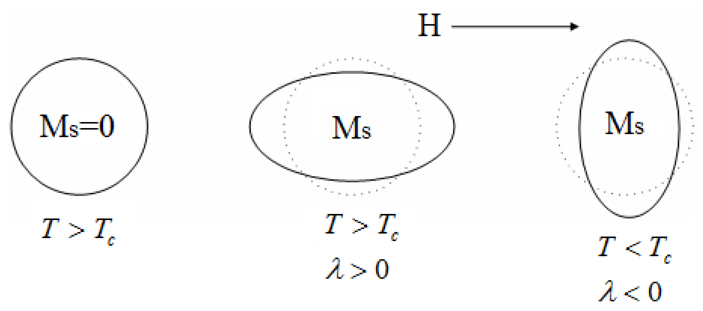
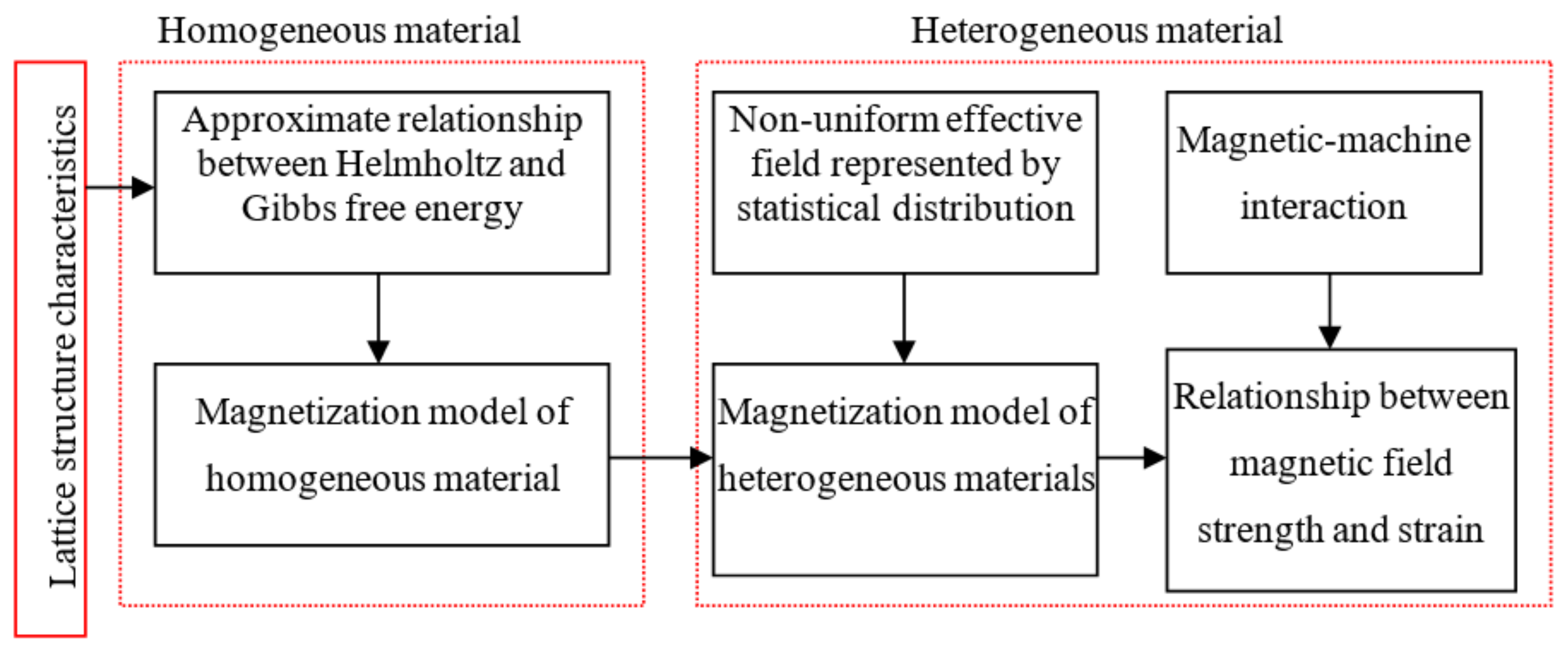
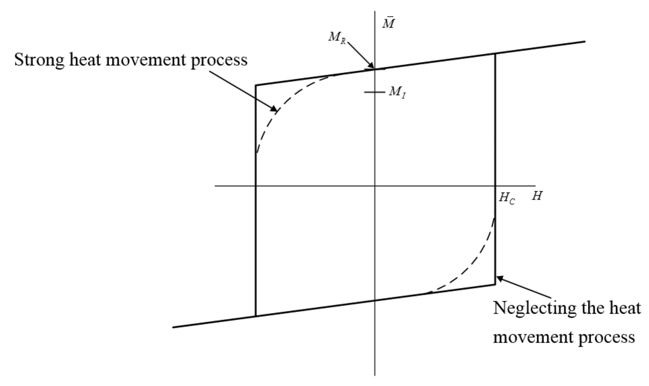
3.1. Research Process Based on the Free Energy Hysteresis Model

The conditions for the free energy hysteresis model are established when the temperature is constant and the influence of eddy current loss is ignored, it works in a low frequency range, the pre-pressure applied to the giant magnetostrictive microactuator is assumed to be large enough to ignore the magnetic anisotropy, and so on. to establish the free energy hysteresis model of the giant magnetostrictive actuator include three steps, the first, the Helmholtz–Gibbs free energy relationship for homogeneous materials with a constant internal field is established, then, the heterogeneity of the actual material and the non-constantness of the internal effective field are considered, and a random distribution function is substituted to derive the hysteresis relationship model between the applied magnetic field strength H and the magnetization M . It is also important to study its magnetic machine coupling characteristics and construct the nonlinear relationship between the applied magnetic field strength H and strain ε . The research process is shown in Figure 2.

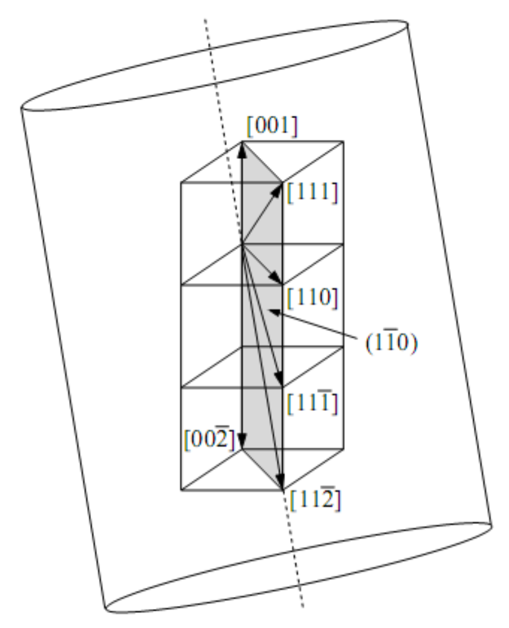
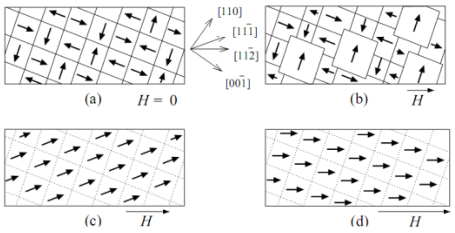
3.2. Theoretical Basis for the Establishment of the Free Energy Hysteresis Model

(1) Magnetization process of the giant magnetostrictive material
In order to establish the energy model of the material, it is necessary to analyze the lattice structure of the material by means of vector representation. In the paper, the symbol ‘()’ represents a plane, the symbol ‘[]’ represents a vector, and the symbol ‘〈 〉’ represents the general name of the series represented by the mark. Therefore, the various planes of the cube are represented as: 100 , 010 , 001 , 1 ¯ 00 , 0 1 ¯ 0 , and 00 1 ¯ , and the direction vector is expressed as: [ 100 ], [ 010 ], [ 001 ], [ 1 ¯ 00 ], [ 0 1 ¯ 0 ], and [ 00 1 ¯ ], among them, 1 ¯ indicates a negative direction.
In the current processing conditions, the lattice of Terfenol-D in the [ 11 2 ¯ ] direction grows in the form of a tree (as shown in Figure 3). In room temperature, the easy magnetization axis of Terfenol-D is generally in the 111 direction series, and the maximum strain occurs when the magnetization M is rotated from direction [111] to [ 11 1 ¯ ] or from direction [ 111 ¯ ] to [ 11 ¯ 1 ].
To take a sample that is not magnetized (as shown in Figure 4). Figure 4a shows that all regions in the specimen been not magnetized have nonzero spontaneous magnetization M 0 . Figure 4b shows that the change in magnetization is mainly caused by the reversible domain wall motion when the input field is low. Figure 4c shows that two irreversible mechanisms are appearanced when the input field gradually increases, which a magnetic domain is increased caused by domain wall movement (consistent with the direction of the magnetic field), and the magnetic moment is rotated to the direction of easy magnetization [ 11 1 ¯ ]. In this phase, inputting a small change in the driving magnetic field produces a large change in magnetization and output mechanical strain. Figure 4d shows that the magnetization saturation state of the material is reached. At this time, the sample can be approximated as a single magnetic domain, and the magnetic moment is completely rotated from the easy magnetization direction to be consistent with the magnetic field direction.
In this study, it is assumed that the pre-stress of the material perpendicular to the direction of the magnetic moment is large enough to dominate the anisotropy of the lattice, then, the magnetization direction of the magnetic domain is easily changed from the original direction 111 to the [111] and [ 1 ¯ 1 ¯ 1 ¯ ] directions perpendicular to the axis [ 11 2 ¯ ]. This can be considered that the output strain is mainly caused by the rotation of the magnetic moment:
λ = 3 2 λ s ( M M s ) 2 ,
where λ s is the saturation magnetostriction rate. M s is the saturation magnetization. M is magnetization. λ is the magnetostriction rate.
In order to simulate the hysteresis behavior of a giant magnetostrictive actuator, the nonlinear relationship between the input magnetic field H and the magnetization M needs to be described quantitatively. Then, Equation (2) is introduced to derive the relationship between the input magnetic field H and the output strain ε .
(2) Description function of Helmholtz and Gibbs energy
To describe the relationship between magnetostatic and magnetoelastic properties of a giant magnetostrictive actuator, it is assumed that free energy is a function of temperature T and other ordered parameters, where e represents magnetization M in magnetostatics and strain ε in magnetoelasticity. The external field is represented by ϕ ˜ and is conjugated with e in thermodynamics. When M is represented by the ordered parameter e , the external field is represented as a magnetic field H . When ε is represented by the ordered parameter e , the external field is represented as stress σ . ψ   ( e , T ) is used to express the general relationship of Helmholtz’s free energy. When no external field is added, the condition of thermodynamic equilibrium is that e is at a minimum, which is:
ϕ ( e , T ) = ψ ( e , T ) e = 0 .
The energy response of the system can be expressed as ϕ . When the system is acted on by the external field ϕ ˜ , total free energy can be expressed as Equation (4):
ψ ϕ ˜ ( e , T ) = ψ ( e , T ) ϕ ˜ e .
The equilibrium conditions applied by an external field are expressed by Equation (5):
ϕ ( e , T ) = ϕ ˜ .
In the case where the pre-pressure is sufficiently large, two magnetization directions in [111] and [ 1 ¯ 1 ¯ 1 ¯ ] in the giant magnetostrictive material will be easily produced. It is necessary to consider both the internal energy and the magnetic moment energy of the material in these two magnetization directions. It is assumed that the interaction between magnetic moments is adiabatic, and the temperature is stable below the Curie temperature, the Helmholtz potential energy ψ can be expressed by Equation (6).
ψ ( M , T ) = H h M s 2 [ 1 ( M / M s ) 2 ] + H h T 2 T c [ M ln ( M + M R M s M ) + M s ln ( 1 ( M / M s ) 2 ) ] ,
where H h is the biasing magnetic field, M s is saturation magnetization, and T c is the Curie temperature.
According to statistical mechanics, Helmholtz free energy can be represented by piecewise quadratic relations under isothermal conditions.
ψ ( M ) = 1 2 η ( M + M R ) 2 , M M I   1 2 η ( M M R ) 2 ,   M M I   1 2 η ( M I M R ) 2 ( M 2 M I M R ) , M < M I ,
where M I is the magnetization generated at the inflection point, M R is residual magnetization, η is the converted slope, and η = d H d M .
By Equation (6), Gibbs energy can be written by Equation (8):
G ( H , M , T ) = ψ ( M , T ) H M .
(3) Hysteresis model of homogeneous material
For homogeneous materials, the effective field H e is equal to the application field H , and the average magnetization can be written by Equation (9).
M ¯ = x M + + + x M ,
where x + / x is the probability of positive or negative magnetic moment, and M + / M is the expected value of magnetization. M + and M can be obtained by Equation (10):
M + = M I M μ ( G ) d M M = M I M μ ( G ) d M
where:
μ ( G ) = C e G V / k T .
The probability of Gibbs energy obtained is expressed quantitatively in the above equation, where k is the Boltzmann constant, C is a constant, and this constant can be selected according to the magnetization integral value 1, V is lattice volume. Considering the Boltzmann energy balance, the approximate relaxation process characteristics of the material can be obtained in the lattice volume V , and then the constant C can be estimated to obtain the average magnetization value.
M + = M I M e G ( H , M ) V / k T d M M I e G ( H , M ) V / k T d M M = M I M e G ( H , M ) V / k T d M M I e G ( H , M ) V / k T d M
According to the normalized equation x + + x = 1 , the matrix component can be quantitatively described by the differential Equation (13).
x ˙ + = p + x + + p + ( 1 x + ) .
The likelihood that the magnetic moment changes from the positive direction to the negative direction is expressed by Equation (14).
p + = 1 Γ ( T ) M I M I e G ( H , M ) V / k T d M M I e G ( H , M ) V / k T d M p + = 1 Γ ( T ) M I M I + e G ( H , M ) V / k T d M M I + e G ( H , M ) V / k T d M
where is constant, Γ is the relaxation time of the material, and ω = 1 Γ , which indicates the frequency of magnetic moment conversion.
In order to qualitatively analyze the model and quantitatively analyze the thermal motion region, it is necessary to simplify the complex behavior of the average magnetization M ¯ in the region where the thermal motion is negligible, according to the equilibrium conditions by Equation (15).
G M = 0 .
Combined with (8), Equation (16) is obtained.
H M = 2 ψ M 2 .
It can be seen from the above equation that the slope of the hysteresis kernel in this linear domain is 1 / η , and the inflection point M I is the key point. At this time, the resilience is the largest, and the original estimated parameter value of the free magnetic hysteresis model of the giant magnetostrictive actuator can be obtained according to the above equilibrium conditions.
In the case where magnetization occurs for a short time and the thermal motion is negligible, the jump will be completed in an instant, so the magnetization can be simplified by an asymptotic relationship (as shown in Figure 5). M min can be obtained by solving Equation (15), and M ¯ = M min , then, M ¯ is calculated.
Combining with the Helmholtz free energy expression (7), the magnetization can be obtained.
[ M ¯ ( H ; H c , ξ ) ] ( t ) = [ M ¯ ( H ; H c , ξ ) ] ( 0 ) , τ ( t ) = ϕ H η M R , τ ( t ) ϕ a n d H [ max τ ( t ) ] = H c H η + M R , τ ( t ) ϕ a n d H [ max τ ( t ) ] = H c ,
When the transition occurs, the set of times τ ( t ) can be expressed by Equation (18).
τ ( t ) = t ( 0 , T f ] | H ( t ) = H c o r H ( t ) = H c .
The initial value of the magnetic moment [ M ¯ ( H ; H c , ξ ) ] ( 0 ) can be expressed by Equation (19).
[ M ¯ ( H ; H c , ξ ) ] ( 0 ) = H η M R , H ( 0 ) H c ξ , H c < H ( 0 ) < H c H η + M R , H ( 0 ) H c .
Coercivity H c can be expressed by Equation (20).
H c = η ( M R M I ) .
(4) Hysteresis model of heterogeneous materials
The magnetization model (Equation (17)) is established on the premise that the internal lattice and magnetic domain structure of the material are completely uniform. In fact, the non-uniformity of the lattice structure of the material is led by the defects of the material itself and the non-uniform free energy profile of its different regions, according to the hypothesis that the effective field H e is equal to the application field H in the homogeneous material, the magnetic interaction and Weiss mean field effect are ignored. To assume that the parameter H c = η ( M R M I ) is a normal distribution, with respect to the average coercivity H ¯ c , the total magnetization can be written by Equation (21).
M ( H ) = 0 M ¯ ( H ; H c , ξ ) f ( H c ) d H c ,
where H c is the density distribution function and can be expressed by Equation (22).
f ( H c ) = C 1 e ( H c H ¯ c ) 2 / b ,
where C 1 and b are coefficients, and M ¯ can be obtained from Equation (10) or (17). In Equation (21), its lower limit of integration is 0, which indicates that the hysteresis core width must be non-negative. In addition, it is defined as a logarithmic function to be also used to reflect the non-negative nature of the hysteresis kernel width.
In the Jiles–Atherton model, the Weiss field effect caused by the coupling between domains can be represented by Equation (23).
H e = H + α M ,
where α is a constant mean field parameter.
Weiss fields quantitatively describe the interaction between atoms in giant magnetostrictive material. The effective field H e exhibits changes caused by uneven magnetic moment distribution, and it is assumed that the effective field H e is a normal distribution of the applied field. The magnetization can be expressed by Equation (24).
M ( H ) = C 2 M ¯ ( Η ; H c , ξ ) e ( H Η ) 2 / b ¯ d Η .
Thus, under the effective field of the low-frequency range without considering the eddy current loss, the complete magnetization model of the heterogeneous polycrystalline material can be expressed as:
[ M ( H ) ] ( t ) = C 0 [ M ¯ ( Η + H ; H c , ξ ) ] ( t ) e Η 2 / b ¯ e ( H c H ¯ c ) 2 / b d Η d H c .
(5) Construction of a magnetic–mechanical coupling eigen model of giant magnetostrictive material
The Gibbs energy expression of Equation (8) combines the internal energy and magnetic moment energy of the isotropic material on the magnitude of the magnetic domain, but the magnetic coupling effect is ignored, and the magnetostrictive ability of the material cannot be exhibited. When anisotropy is exhibited for the lattice dominated by the actuator’s pre-stress, the Helmholtz free energy relation embodying magnetoelasticity can be expressed by Equation (26).
ψ e ( M , ε ) = ψ ( M ) + 1 2 Y M ε 2 Y M γ ε M 2 .
The corresponding Gibbs energy is expressed by Equation (27).
G ( H , M , ε ) = ψ ( M ) + 1 2 Y M ε 2 Y M γ ε M 2 H M σ ε ,
where ψ can be obtained from Equation (7). Y M is the Young’s modulus at a certain magnetization. γ is the magnetic coupling coefficient.
In the case of intense thermal motion, the magnetization M ¯ can be obtained by Equation (9), and the Gibbs energy can be obtained by Equation (27). Magnetization is expressed by Equation (28) when the thermal motion is ignored.
[ M ¯ ( H , ε ; H c , ξ ) ] ( t ) = [ M ¯ ( H , ε ; H c , ξ ) ] ( 0 ) , τ ( t ) = ϕ H η 2 Y M γ ε M R η η 2 Y M γ ε , τ ( t ) ϕ a n d H [ max τ ( t ) ] = H c H η 2 Y M γ ε + M R η η 2 Y M γ ε , τ ( t ) ϕ a n d H [ max τ ( t ) ] = H c ,
where H c = η ( M R M I ) , τ ( t ) can be obtained by Equation (18), and Equation (29) is obtained.
[ M ¯ ( H , ε ; H c , ξ ) ] ( 0 ) = H η 2 Y M γ ε M R η η 2 Y M γ ε , H ( 0 ) H c ξ , H c < H ( 0 ) < H c H η 2 Y M γ ε + M R η η 2 Y M γ ε , H ( 0 ) H c .
The equilibrium condition of the elastic constitutive relation is expressed by Equation (30).
G ε = 0 .
Then:
σ = ψ e ε M .
For undamped magnetostrictive material, the magnetic–mechanical coupling constitutive relation can be expressed by Equations (32) and (33).
σ = Y M ε Y M γ M 2 ,
M ( H , ε ) = C 0 M ¯ ( Η + H , ε ; H c , ξ ) e Η 2 / b ¯ e ( H c H ¯ c ) 2 / b d Η d H c .
When the thermal motion is neglected, M ¯ can be obtained from Equation (28). When the strong thermal motion or relaxation mechanism is considered, M ¯ can be derived from Equation (9) and can be obtained by Equation (27).

4. Numerical Implementation of a Magnetization Model Based on the Free Energy Hysteresis Model

According to reference [43], the model is constructed with the piecewise linear kernel function. In order to achieve the highest calculation accuracy and the fastest efficiency, during the numerical solution of the free energy hysteresis model, the Gauss–Legendre algorithm is used to discretize the integral, and the kernel function is realized by using the matrix representation.

4.1. Discretization of Integrals

Divide the integral limit of Equation (25) into a limited number of cells Ω 2 , and the Gauss–Legendre method is applied to discrete each integration interval. The general form of the Gauss–Legendre algorithm is:
1 1 f ( x ) d x = A k f ( x k ) .
Then, the numerical equation of the free energy magnetization model can be written by Equation (35).
[ M ( H ) ] ( t ) = i = 1 N i j = 1 N j υ 1 ( H c i ) υ 2 ( Η j ) [ M ¯ ( Η j + H ; H c i , ξ i ) ] v i w j ,
where υ 1 ( H c i ) = c 1 e ( H c i H c ¯ ) 2 / b , υ 2 ( Η j ) = c 2 e Η j 2 / b ¯ , H c i and Η j are Gaussian integration points, and v i and w j are weight functions.
The original discretized equation can be transformed into Equation (36).
[ M ( H ) ] ( t ) = C i = 1 N i j = 1 N j e ( H c i H c ¯ ) 2 / b e Η j 2 / b ¯ [ M ¯ ( Η j + H ; H c i , ξ i ) ] v i w j .

4.2. Kernel Function Implementation

According to Equation (17), the piecewise linear equation of the local magnetization can be described by Equation (37) in the case of where thermal motion is ignored.
M ¯ = H η + M R Δ ,
where, when Δ = 1 , magnetization is located on the upper branch of the kernel function here, and when Δ = 1 , magnetization is located on the lower branch of the kernel function here (as shown in Figure 6).
In order to accurately represent the judgment conditions of the Equation (37), and the calculation speed is improved effectively, a matrix algorithm is used, as defined by Equation (38).
Δ int = - 1 - 1 - 1 - 1 1 1 1 1 N i × N j H c = H c 1 H c 1 H c N i H c N i N i × N j h k = H k + 1 H k + N j H k + 1 H k + N j N i × N j
The weight function vector is defined by Equation (39).
V T = v 1 υ 1 ( H c 1 ) v N i υ 1 ( H c N i ) 1 × N i W T = w 1 υ 2 ( Η 1 ) w N j υ 1 ( Η N j ) 1 × N j
According to the magnetic field strength value H k , magnetization M k = M ( H k ) , and it can be calculated by the following algorithm:
d H = H k H k 1 h k = h k + d H   Δ = s i g n ( h k + H c Δ )   M ¯ = h k η + M R Δ M k = V T M ¯ W ,
where H k is the value of the magnetic field strength corresponding to the k element after discretization, h k is the effective field, the i j element in the   Δ constructed matrix indicates whether the j effective field just crosses the i critical magnetic field strength, and H c is the critical magnetic field strength.

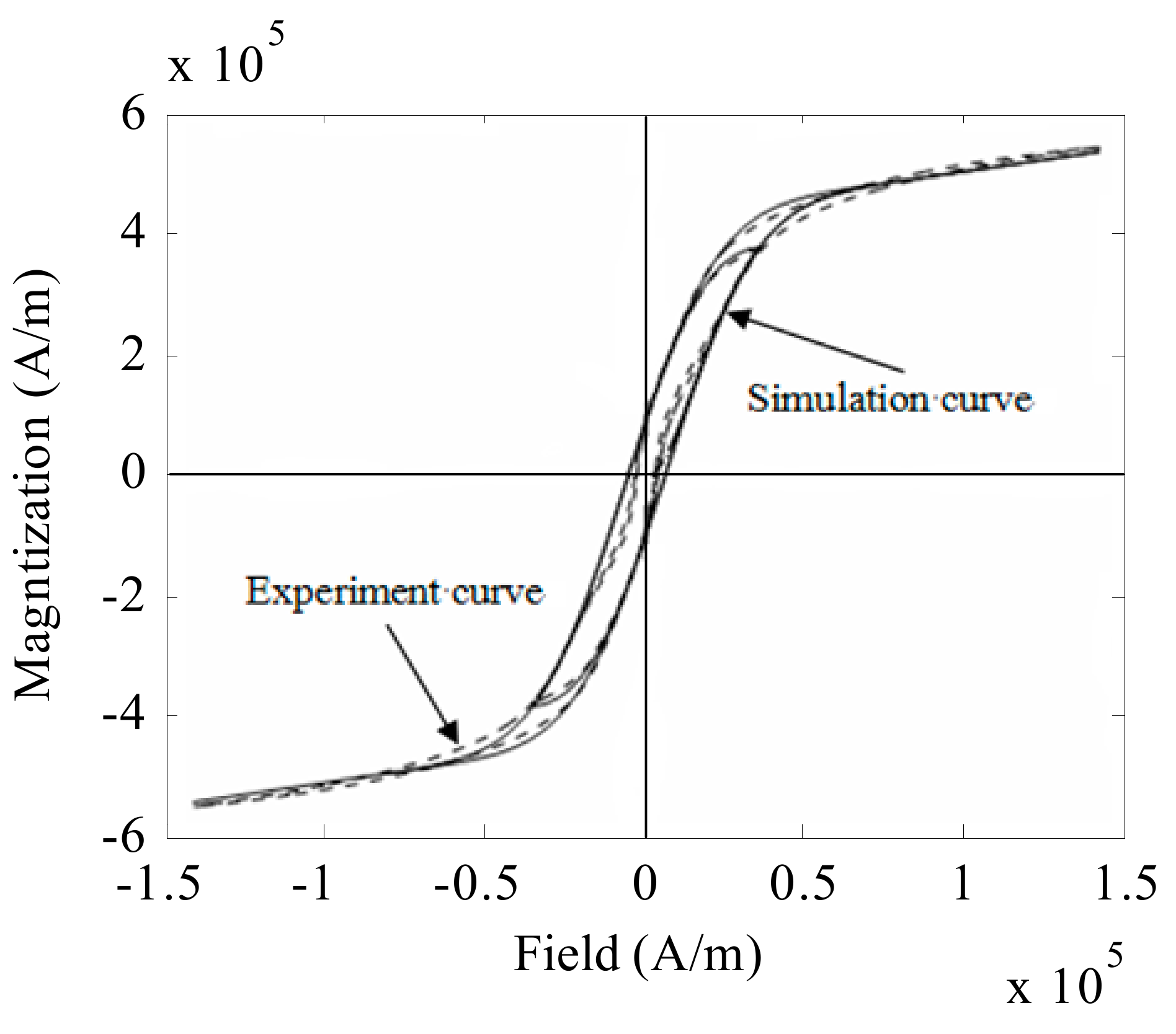
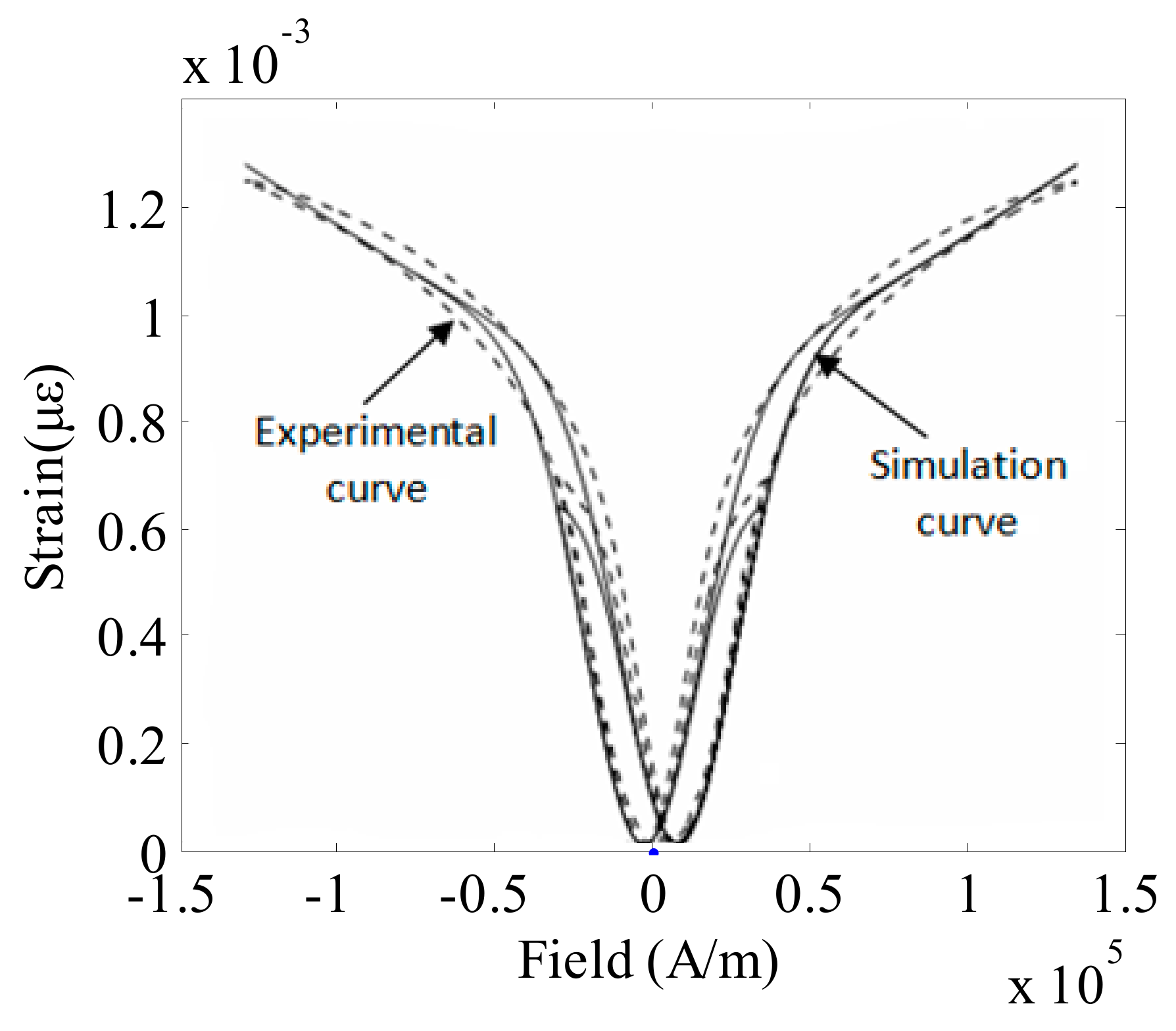
4.3. Verification Based on the Free Energy Hysteresis Model

To verify the correctness of the numerical implementation method based on the free energy hysteresis model, the parameters of [41] are used to analyze: M R   =   3.7   ×   10 4 A / m , η = 14 , H c = 300 A / m , b   =   1   ×   10 8 A 2 / m 2 , b ¯   = 8   ×   10 8 A 2 / m 2 , C   =   2.52   ×   10 8 , and γ   =   4.5   ×   10 15 m 2 / A 2 (the specific parameters of different giant magnetostrictive actuators can be estimated by the least-squares method). Assuming the pre-pressure is constant, the magnetic anisotropy considered in Equation (36) can be ignored. Then, ε = 0 in Equation (28), and the measured strain can be solved.
In the period of the input field, it is proposed to take 200 breakpoints for calculation, the relationship between the output magnetization M , the output displacement σ , and the input magnetic field strength H is shown in Figure 6 and Figure 7, respectively. The calculation results of the magnetic machine coupling model in the original reference [41] are shown in Figure 8 and Figure 9. When the two figures are compared, it can be seen that the calculation results are consistent with the simulation results in reference [41].

5. Conclusions

The dynamic magneto-mechanical coupling model of a giant magnetostrictive actuator based on its intrinsic nonlinearity and hysteresis effect is an important theoretical basis for designing GMAs, predicting the displacement output of GMAs, and to provide a reliable basis for GMA system design. The hysteresis characteristics and nonlinearity of giant magnetostrictive actuators have been researched intensively based on the theoretical study of the free energy hysteresis model in this paper. The magnetization model of homogeneous material is derived according to the expression of Helmholtz and Gibbs energy, and two extensions are carried out to obtain the magnetization model of the heterogeneous material. Finally, the magnetic–mechanical coupling constitutive relation of the magnetic field strength H and strain ε is obtained, which is driven from magneto-mechanical coupling effects. Then, the Gauss–Legendre method is used to discretize the integral, the kernel function is realized by using the matrix representation, and the numerical realization of the free energy magnetization model is derived. Reliable experimental data were selected as parameters to verify the free energy magnetization model, and the simulation results are consistent with the existing experimental results. The results show that they are correct for the magnetization model based on the hysteresis characteristics of free energy and its numerical implementation, and the research results provide a theoretical basis for the engineering application of giant magnetostrictive material and the optimization of micro-actuator structures of giant magnetostrictive material.

Author Contributions

Conceptualization, Z.Y. and M.Z.; Methodology, Z.Y. and C.-y.Z.; Validation, Z.Y., Z.D. and M.Z.; Formal Analysis, M.Z. and Z.D.; Investigation, C.-y.Z. and J.-x.Y.; Resources, Z.Y.; Data Curation, Z.D., M.Z. and J.-x.Y.; Writing-Original Draft Preparation, Z.Y.; Writing-Review & Editing, Z.Y.; Supervision, Z.Y.; Project Administration, Z.Y.; Funding Acquisition, Z.Y. and Z.D.

Funding

The research is funded by National Natural Science Fund (Grant No.51475339), Natural Science Fund of Hubei Province (Grant No. 2016CFB581), and Key Laboratory Open Fund of Ministry of Education of Metallurgical Equipment and Control of Wuhan University of Science and Technology (2013A07).

Conflicts of Interest

The authors declare no conflict of interest.

References

  1. Jia, Z.Y.; Wang, F.J.; Guo, D.M. Functional Material Driving Microactutor and Its Key Technology. Chin. J. Mech. Eng. 2003, 39, 61–67. [Google Scholar] [CrossRef]
  2. Lu, Q.G. Development and application of micro actuation technology. J. Nanchang Inst. 2008, 12, 1–6. [Google Scholar]
  3. Park, G.; Bement, M.T.; Hartman, D.A.; Smith, R.E.; Farrar, C.R. The use of active materials for machining processs: A review. Int. J. Mach. Tools Manuf. 2007, 47, 2189–2206. [Google Scholar] [CrossRef]
  4. Liang, S.Y.; Hecker, R.L.; Landers, R.G. Machining process monitoring and control: The state of the art, ASME. J. Manuf. Sci. Eng. 2004, 126, 297–310. [Google Scholar] [CrossRef]
  5. Inman, D.J. Smart materials in damage detection and prognosis. In Proceedings of the Fifth International Conference on Damage Assessment of Structures, Southampton, UK, 1–3 July 2003; pp. 3–16. [Google Scholar]
  6. Maffiodo, D.; Raparelli, T. Flexible Fingers Based on Shape Memory Alloy Actuated Modules. Machines 2019, 7, 36–40. [Google Scholar] [CrossRef]
  7. Khan, M.M.; Lagoudas, D.C.; Rediniotis, O.K. Thermoelectric SMA actuator: Preliminary prototype testing. Proc. Spie-Int. Soc. Opt. Eng. 2004, 113, 94–99. [Google Scholar]
  8. Ohmata, K.; Zaike, M.; Koh, T. A Three-link Arm Type Vibration Control Device Using Magnetostrictive Actuators. J. Alloy. Compd. 1997, 258, 74–78. [Google Scholar] [CrossRef]
  9. Wakiwaka, H.; Aoki, K.; Yoshikawa, T.; Kamata, H.; Igarashi, M.; Yamada, H. Maximum output of a low frequency sound source using giant magnetostrictive material. J. Alloy. Compd. 1997, 258, 87–92. [Google Scholar] [CrossRef]
  10. Jenner, A.G.; Smith, R.J.E.; Wilkinson, A.J. Actuation and transduction giant magnetostrictive alloys. Mechatronics 2000, 10, 457–466. [Google Scholar] [CrossRef]
  11. Li, Q.; Ye, Z.; Meng, Y.; Tian, Y.; Wen, S. Linear inchworm mechanism based on giant magnetostrictive and piezoelectric materials. J. Tsinghua Univ. (Sci. Technol.) 2005, 45, 1055–1057. [Google Scholar]
  12. Clark, A.E. Magnetostrictive Rare Earth-Fe2 Compounds; Wohlfarh, E.P., Ed.; North-Holland Publishing Company: New York, NY, USA, 1980. [Google Scholar]
  13. Benbouzid, M.E.H.; Reyne, G.; Meunier, G.; Kvarnsjo, L.; Engdahl, G. Dynamic modelling of giant magnetostriction in Terfenol-D rods by the finite element method. IEEE Trans. Magn. 1995, 31, 1821–1824. [Google Scholar] [CrossRef]
  14. Azoum, K.; Besbes, M.; Bouillault, F. 3D FEM of magnetostriction phenomena using coupled constitutive laws. Int. J. Appl. Electromagn. Mech. 2004, 19, 367–371. [Google Scholar] [CrossRef]
  15. Benatar, J.G. Fem implementations of magnetostrictive-based applications. Master’s Thesis, University Of Maryland, College Park, MD, USA, 2005. [Google Scholar]
  16. Zhao, Z.; Wu, Y.; Gu, X. Three-dimensional nonlinear dynamic finite element model for giant magnetostrictive actuators. J. Zhgenjiang Univ. (Eng. Sci.) 2008, 2, 203–208. [Google Scholar]
  17. Zhong, W.-D. Ferromagnetics (Version 2); Science Press: Beijing, China, 1992. [Google Scholar]
  18. De Lacheisserie, E.D.T. Magnetostriction Theory and Applications of Magnetoelasticity; CRC Press, Inc.: Boca Raton, FL, USA, 1993. [Google Scholar]
  19. Wang, S.; Wan, F.; Zhao, H.; Chen, W.; Zhang, W.; Zhou, Q. A Sensitivity-enhanced Fiber Grating Current Sensor Based on Giant Magnetostrictive Material for Large-Current Measurement. Sensors 2019, 19, 1755. [Google Scholar] [CrossRef]
  20. Mcmaster, O.D.; Verhoeven, J.B.; Gibson, E.D. Preparation of Terfenol-D by Float Zone Solidification. J. Magn. Magn. Mater. 1986, 54, 849–851. [Google Scholar] [CrossRef]
  21. Tang, X.; Miao, Y.; Chen, X.; Nie, B. A Flexible and Highly Sensitive Inductive Pressure Sensor Array Based on Ferrite Films. Sensors 2019, 19, 2406. [Google Scholar] [CrossRef]
  22. Greenough, R.D.; Sehulze, M.P.; Pollard, D. Non-destructive testing of Terfenol-D. J. Alloy. Compd. 1997, 258, 118–122. [Google Scholar] [CrossRef]
  23. Claeyssen, F.; Lhermet, N.; Le Letty, R.; Bouchilloux, P. Actuators transducers and motors based on giant magnetostrictive materials. J. Alloy. Compd. 1997, 258, 61–73. [Google Scholar] [CrossRef]
  24. Moffett, M.B.; Clark, A.E.; Wun-Fogle, M.; Linberg, J.; Teter, J.P.; McLaughlin, E.A. Characterization of Terfenol-D for magnetostrictive transucers. J. Acoust. Soc. Am. 1991, 89, 1448–1455. [Google Scholar] [CrossRef]
  25. MOHRI, K. Factors Affecting the Output Voltage of a Magnetostrictive Torque Sensor Constructed from Ni-Fe Sputtered Films and a Ti-Alloy Shaft. Jpn. Appl. Magn. Soc. 1998, 22, 1074–1079. [Google Scholar]
  26. Hall, A.; Coatney, M.; Bradley, N.; Hyeong Yoo, J.; Jones, N.; Williams, B.; Myers, O. Nondestructive Damage Detection of a Magnetostrictive Composite Structure. Proceedings 2018, 2, 416. [Google Scholar] [CrossRef]
  27. Stovner, B.N.; Johansen, T.A.; Schjølberg, I. Globally exponentially stable filters for underwater position estimation using an array of hydroacoustic transducers on the vehicle and a single transponder. Ocean Eng. 2018, 155, 351–360. [Google Scholar] [CrossRef]
  28. Clark, A.E.; Teter, J.P.; McMasters, D. Magnetostriction jumps in twined Tb0.3Dy0.7Fe1.9. J. Appl. Phys. 1988, 63, 3910–3912. [Google Scholar] [CrossRef]
  29. Choudhary, P.; Meydan, T. A novel aceelerometer design using the inverse magnetostrictive effect. Sens. Actuators 1997, 59, 51–55. [Google Scholar] [CrossRef]
  30. Ishihara, S. High Precision Positioning for Submicron Lithography Bull. Jpn. Soc. Pree 1987, 21, 1–8. [Google Scholar]
  31. Tatevosyan, A.S.; Tatevosyan, A.A.; Zaharova, N.V. The Study of the Electrical Steel and Amorphous Ferromagnets Magnetic Properties. Procedia Eng. 2016, 152, 727–734. [Google Scholar] [CrossRef]
  32. Apicella, V.; Clemente, C.S.; Davino, D.; Leone, D.; Visone, C. Review of Modeling and Control of Magnetostrictive Actuators. Actuators 2019, 8, 45. [Google Scholar] [CrossRef]
  33. Iyer, R.V.; Tan, X.; Krishnaprasad, P.S. Approximate Inversion of the Preisach Hysteresis Operator with Application to Control of Smart Actuators. IEEE Trans. Autom. Control 2005, 50, 798–810. [Google Scholar] [CrossRef]
  34. Tan, X.; Baras, J.S.; Krishnaprasad, P.S. A dynamic model for magnetostrictive hysteresis. In Proceedings of the 2003 American Control Conference, Denver, CO, USA, 4–6 June 2003; Volume 2, pp. 1074–1079. [Google Scholar]
  35. Mayergoyz, I.D.; Friedman, G. Generalized Preisach Model of Hysteresis. IEEE Trans. Magn. 1988, 24, 212–217. [Google Scholar] [CrossRef]
  36. Della Torre, E. Preisach modeling and reversible magnetization. IEEE Trans. Magn. 1990, 26, 3052–3058. [Google Scholar] [CrossRef]
  37. Yu, Y.; Li, J.; Li, Y.; Li, S.; Li, H.; Wang, W. Comparative Investigation of Phenomenological Modeling for Hysteresis Responses of Magnetorheological Elastomer Devices. Int. J. Mol. Sci. 2019, 20, 3216. [Google Scholar] [CrossRef]
  38. Jiles, D.C. Introduction to Magnetism and Magnetic Materials; Chapman and Hall: London, UK, 1995. [Google Scholar]
  39. Dapino, M.J.; Smith, R.C.; Flatau, A.B. Structural Magnetic Strain Model for Magneto-strictive Transducers. IEEE Trans. Magn. 2000, 36, 545–556. [Google Scholar] [CrossRef]
  40. Smith, R.C.; Dapino, M.J.; Seelecke, S. Free energy model for hysteresis in magnetostrictive transducers. J. Appl. Phys. 2003, 93, 458–466. [Google Scholar] [CrossRef] [Green Version]
  41. Smith Ralph, C.; Dapino Marcelo, J.; Braun Thomas, R.; Mortensen Anthony, P. A homogenized energy framework for ferromagnetic hysteresis. IEEE Trans. Magn. 2006, 42, 1747–1769. [Google Scholar] [CrossRef]
  42. Smith, R.C.; Seelecke, S.; Dapino, M.; Ounaies, Z. A unified framework for modeling hysteresis in ferroic materials. J. Mech. Phys. Solids 2006, 54, 6–85. [Google Scholar] [CrossRef]
  43. Xiao, Y.; Gou, X.F.; Zhang, D.G. A one-dimension nonlinear hysteretic constitutive model with elasto-thermo-magnetic coupling for giant magnetostrictivematerials. J. Magn. Magn. Mater. 2017, 441, 642–649. [Google Scholar] [CrossRef]
Figure 1. Spontaneous deformation diagram.
Applsci 09 03691 g001
Figure 2. Free energy hysteresis model construction process.
Applsci 09 03691 g002
Figure 3. Lattice direction representation of Terfenol-D.
Applsci 09 03691 g003
Figure 4. The magnetization process of plane 1 1 ¯ 0 of the Terfenol-D single crystal under the magnetic field in the [ 11 2 ¯ ] direction. (a) Non-zero spontaneous magnetization state; (b) Magnetization caused by the reversible domain wall motion when the input field is low; (c) Two irreversible magnetization mechanisms appearanced when the input field increases gradually; (d) The magnetization saturation state of the material.
Applsci 09 03691 g004
Figure 5. Relationship between magnetization M ¯ and magnetic field strength H .
Applsci 09 03691 g005
Figure 6. Simulation curve of magnetization and magnetic field strength.
Applsci 09 03691 g006
Figure 7. Simulation curve of output displacement and magnetic field strength.
Applsci 09 03691 g007
Figure 8. Simulation and experimental comparison curves of magnetization and magnetic field strength.
Applsci 09 03691 g008
Figure 9. Simulation and experimental comparison curves of output displacement and magnetic field strength.
Applsci 09 03691 g009

