Article

A Deep Belief Network Combined with Modified Grey Wolf Optimization Algorithm for PM2.5 Concentration Prediction

1
College of Earth Sciences and Engineering, Hohai University, Nanjing 211100, China
2
College of Automation Engineering, Nanjing University of Aeronautics and Astronautics, Nanjing 211106, China
3
College of Geodesy and Geomatics, Wuhan University, Wuhan 430079, China
4
College of Geography and Information Engineering, China University of Geosciences, Wuhan 430074, China
*
Author to whom correspondence should be addressed.
Submission received: 1 August 2019 / Revised: 6 September 2019 / Accepted: 6 September 2019 / Published: 9 September 2019
(This article belongs to the Special Issue Air Pollution)

Abstract

:
Accurate PM2.5 concentration prediction is crucial for protecting public health and improving air quality. As a popular deep learning model, deep belief network (DBN) for PM2.5 concentration prediction has received increasing attention due to its effectiveness. However, the DBN structure parameters that have a significant impact on prediction accuracy and computation time are hard to be determined. To address this issue, a modified grey wolf optimization (MGWO) algorithm is proposed to optimize the DBN structure parameters containing number of hidden nodes, learning rate, and momentum coefficient. The methodology modifies the basic grey wolf optimization (GWO) algorithm using the nonlinear convergence and position update strategies, and then utilizes the training error of the DBN to calculate the fitness function of the MGWO algorithm. Through the multiple iterations, the optimal structure parameters are obtained, and a suitable predictor is finally generated. The proposed prediction model is validated on a real application case. Compared with the other prediction models, experimental results show that the proposed model has a simpler structure but higher prediction accuracy.

1. Introduction

With continuous advancement of industrialization and urbanization, artificial pollutants such as industrial production and automobile exhaust are increasing. As a consequence, urban air quality has gradually deteriorated, which seriously affects people’s living environment. PM2.5, as one of the main pollutants in urban atmosphere has a small particle size, allowing staying in the atmosphere for a long time. It can enter human body through breathing and then deposits in the alveoli, causing great harm to human body [1]. Besides, PM2.5 has a negative impact on atmospheric visibility and climate change [2]. Therefore, accurate PM2.5 concentration prediction is necessary for controlling air pollution and protecting human health.
Early prediction methods of PM2.5 concentration are mostly simple regression analysis. The regression equation between influencing factors and pollutant is established [3,4,5]. Subsequently, back-propagation (BP) neural network [6,7], support vector machine (SVM) [8,9], and other machine learning prediction methods are developed for the concentration prediction. However, these traditional machine learning methods are hard to learn the intrinsic relationship between the influencing factors and pollutant due to the shallow learning. In terms of prediction accuracy, it is not satisfactory.
In 2006, Hinton et al. proposed a deep learning model, so-called deep belief network (DBN) [10]. It consists of multiple restricted Boltzmann machines (RBMs) and a back propagation (BP) neural network, allowing processing large amounts of data. In recent decades, the DBN has been successfully applied to fault diagnosis, wind speed forecasting, breast cancer classification, and so on [11,12,13,14,15,16]. Due to its advantage in prediction accuracy, in this paper, we introduce the DBN to conduct the PM2.5 concentration prediction. However, how to determine the structure parameters is an important issue when building a DBN network for PM2.5 concentration. The unsatisfactory network structure parameters—which contain number of hidden nodes, learning rate, and momentum coefficient—will reduce the prediction accuracy and increase the calculation time.
This paper aims to establish a prediction model with high accuracy for PM2.5 concentration. Main contributions are as follows:
  • An advanced deep learning model, so-called DBN, is introduced to predict the PM2.5 concentration, which establishes the close relationship between the influencing factors and pollutant.
  • A modified grey wolf optimization (MGWO) algorithm is proposed to determine the DBN structure parameters, which improves the prediction accuracy of PM2.5 concentration and reduces the computation time.
  • The proposed model is successfully applied to the PM2.5 concentration prediction of Baoding city in China where air pollution is particularly serious.
The rest of this paper is organized as follows. Section 2 is devoted to the description of the DBN and the MGWO algorithm, including how to construct their combination. Section 3 presents the data source and the process of model establishment. Besides, several experiments have been done to validate the effectiveness and superiority of the proposed prediction model. In Section 4, the concluding remarks and future work are given.

2. PM2.5 Concentration Prediction Approach

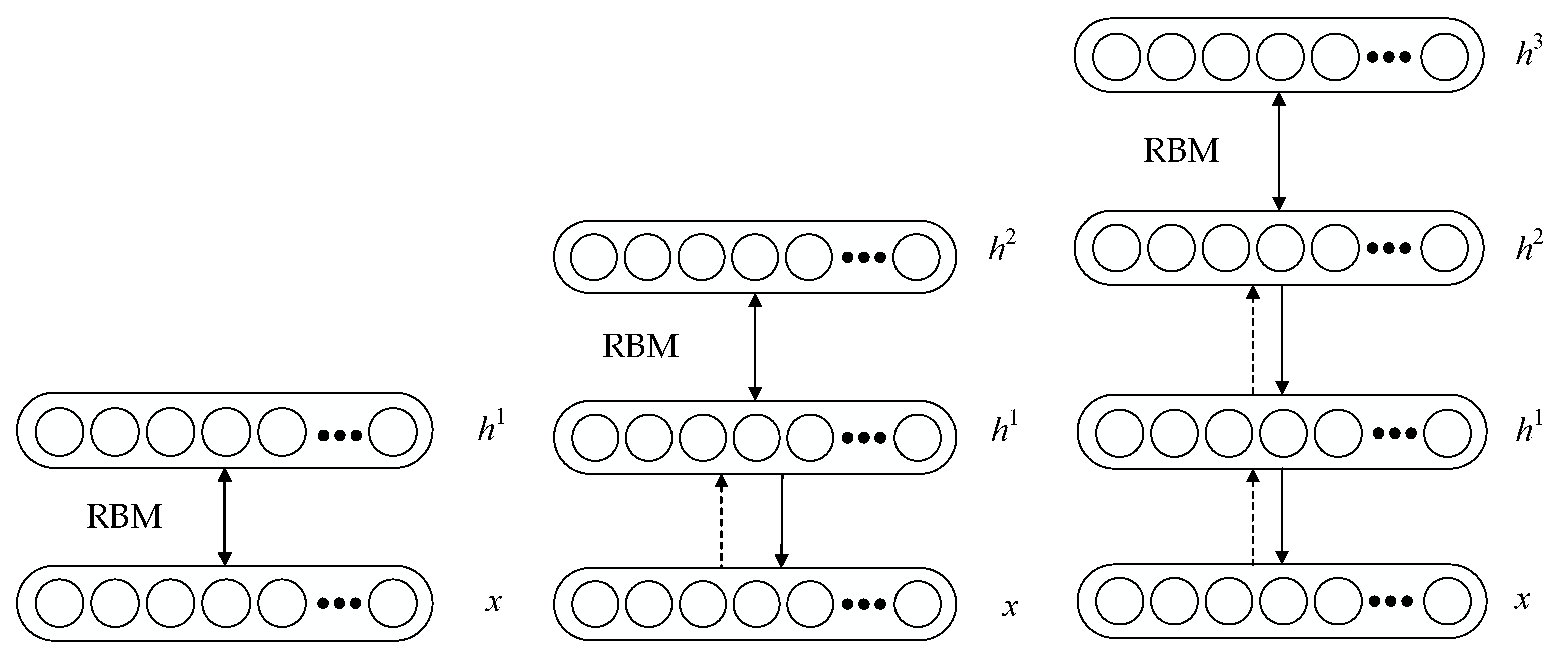
2.1. Deep Belief Network

Deep belief network (DBN) is a probability generation model with multiple hidden layers. It maximizes the generation probability of entire model by training weights between nodes. Figure 1 shows the basic structure of the DBN. It consists of several restricted Boltzmann machines (RBMs) and a back propagation (BP) neural network. RBM, whose output is fed into the input of the next RBM, is a two-layer neural network with directional connections. Thus, a multi-hidden layer structure can be continuously superimposed.
Figure 2 shows the basic structure of the RBM. Wherein v i and h i are the visible and hidden nodes of the input and output layers, respectively. The visible and hidden nodes are fully connected in both directions, while there is no connection between them. b and c denote the biases of the output and input layers respectively, while w denotes the connection weight between the visible node and the hidden node. Thus, the model parameter set θ consists of b , c , and w.
The energy function of the RBM is defined as
E ( v , h ) = i = 1 m v 1 c i j = 1 n h j b j i = 1 m j = 1 n v i h j w i j
Then, the joint probability distribution function of the visible and hidden nodes can be obtained by the energy function.
P ( v , h | θ ) = 1 Z ( θ ) e E ( v , h | θ )
Z ( θ ) = v , h e E ( v , h | θ )
where Z ( θ ) is a partition function for normalization.
In the RBM, given the input vector v , the activation probability of the hidden node h i of the output layer can be expressed as
P ( h i = 1 ) = 1 1 + exp ( b j i v i w i j )
Given the output vector h , the activation probability of the visible node v i of the input layer can be expressed as
P ( v i = 1 ) = 1 1 + exp ( c j j h j w j i )
To obtain the optimal solution of the model, the negative log-likelihood function of training set D is taken as the loss function and is given by
l ( θ , D ) = 1 N v ( i ) D log P ( v ( i ) )
where N is the size of the training set. After that, each weight is updated by the partial derivatives of the loss function for parameter set θ , as follows.
log p ( v ; θ ) w i j = v i h j d v i h j m log p ( v ; θ ) b = h j d h j m log p ( v ; θ ) c = v i d v i m }
where < : > d denotes the statistical probability of the samples, and < : > m denotes the generation probability of the model. Through adjusting the weights of each node, DBN makes the statistical probability of the samples equal to the generation probability of the model as much as possible.
The training process of the DBN is divided into two stages. The first stage is to train each RBM from bottom up. The second stage is to fine-tune the network parameters from top down. In the RBM, the unbiased statistical probability of the samples can be calculated using Equations (4) and (5), while the unbiased generation probability of the model is difficult to obtain. To address this issue, Hinton proposed a contrast divergence algorithm [17] to obtain an approximation of the RBM distribution by one Gibbs sampling. The process can be described mathematically as
w n λ w n 1 + σ ( v i h j 0 v i h j 1 ) b n λ b n 1 + σ ( v h j 0 h j 1 ) c n λ c n 1 + σ ( v i 0 v i 1 ) }
where σ and λ denote the learning rate and the momentum coefficient, respectively.

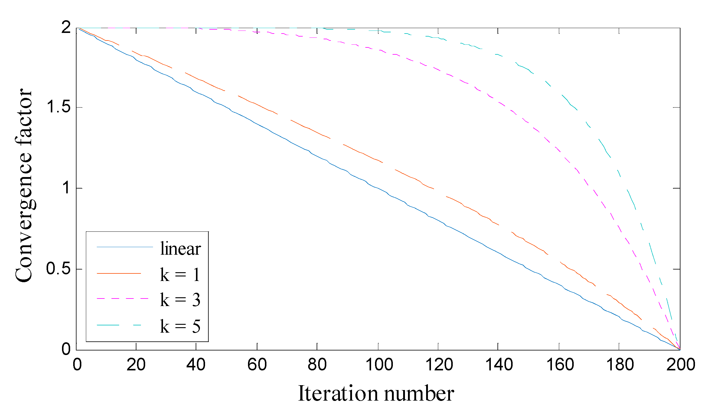
2.2. Modified Grey Wolf Optimization Algorithm

Grey wolf optimization (GWO) algorithm [18] simulates intelligent hunting behavior of grey wolves. According to hierarchical mechanism, grey wolf population can be divided into chief wolf α , deputy chief wolf β , ordinary wolf δ , and bottom wolf ω from high to low. When the wolves capture prey, the other individuals are organized to besiege the prey under the leadership of wolf α . In the GWO algorithm, the α , β , and δ denote the individuals with best fitness, the second best fitness and the third best fitness respectively, while the remaining individuals are noted as ω . The position of the prey is defined as the global optimal solution of optimization problem. Then, the GWO algorithm can be briefly described as follows.
In a D-dimensional search space, suppose that the position of the i th grey wolf is X i = ( X i 1 , X i 2 , , X i d , , X i D ) , where X i d denotes the position of the i th grey wolf in the d th dimension. First of all, the grey wolf population surrounds the prey. The mathematical description of the process is
X i d ( t + 1 ) = X p d ( t ) A i d | C i d X p d ( t ) X i d ( t ) |
where t is the current number of iterations; X p = ( X p 1 , X p 2 , , X p D ) is the prey position; A i d | C i d X p d ( t ) X i d ( t ) | is the surrounding step; and the coefficient vectors A i d and C i d are given by
A i d = 2 a r 1 a
C i d = 2 r 2
where r 1 and r 2 denote the random variables between [0, 1]; and a is the convergence factor. In the evolution process of the algorithm, the convergence factor a changes with the current number of the iterations and is given by
a = 2 2 t T
where T is the maximum number of the iterations. Obviously, the convergence factor a decreases from 2 to 0 as t increases, which serves as the global search and local search for the adjustment of the algorithm.
Next, the grey wolf population hunts. The process, which is guided by α , β , and δ , aims to update the all individual positions. The mathematical description is
X i , α d ( t + 1 ) = X α d ( t ) A i , 1 d | C i , 1 d X α d ( t ) X i d ( t ) | X i , β d ( t + 1 ) = X β d ( t ) A i , 2 d | C i , 2 d X β d ( t ) X i d ( t ) | X i , δ d ( t + 1 ) = X δ d ( t ) A i , 3 d | C i , 3 d X δ d ( t ) X i d ( t ) | }
X i d ( t + 1 ) = X i , α d ( t + 1 ) + X i , β d ( t + 1 ) + X i , δ d ( t + 1 ) 3
Finally, the grey wolves attack and capture the prey. The attack behavior is mainly achieved by linearly decreasing the convergence factor a from 2 to 0. When | A | 1 , the grey wolves concentrate on attacking the prey, corresponding to the local search of the algorithm, while when | A | > 1 , the grey wolves disperse for the global search.
How to balance the local search and the global search is a very important problem often encountered in swarm intelligence algorithm [19]. The local search ability can speed up the convergence of the algorithm; while the global search can maintain the diversity of the population. For the GWO algorithm, we find that the convergence process in practice is not linear. Instead, a nonlinear convergence factor may be more appropriate for balancing the local search and the global search. Thus, a new nonlinear convergence factor is proposed to replace the original linear convergence factor (Equation (12)) and is given by
a = 2 2 ( tan ( π t 4 T ) ) k
where k denotes the attenuation order of the nonlinear convergent factor and takes the integer between 0 and 5. The nonlinear convergence factor with larger k decreases more sharply. Figure 3 shows the convergence factors with different values of k . At the beginning of the iterations, the attenuation degree of a is reduced for constructing the global search. In the later stage of the iterations, the attenuation degree of a is improved for constructing the local accurate search. In this paper, value of k is taken as 3.
The original GWO algorithm updates the grey wolf positions through calculating the average of the three best grey wolf positions. However, the update strategy ignores the characteristics of the different solutions, which may achieve the final solution with lower accuracy. In this paper, we design a weighting factor considering the contribution of each solution. Thus, Equation (14) is modified as
X i d ( t + 1 ) = w α X i , α d ( t + 1 ) + w β X i , β d ( t + 1 ) + w δ X i , δ d ( t + 1 )
w i = 1 / f i 1 / f α + 1 / f β + 1 / f δ , i = α , β , δ
where f α , f β , and f δ denote the values of the fitness of α , β , and δ , respectively; and w α , w β , and w δ denote the values of the weighting factor of α , β , and δ , respectively.

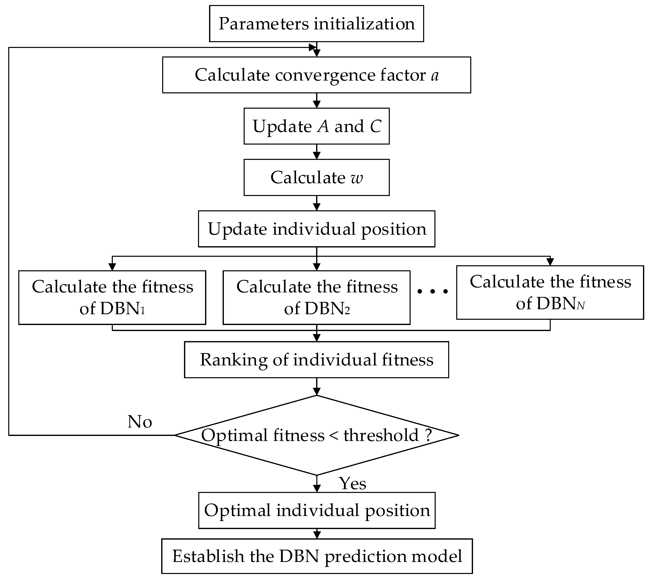
2.3. DBN Structure Parameters Determined by MGWO Algorithm

Due to lack of the effective training algorithms for the DBN structure parameters containing the number of hidden layers, the number of hidden nodes, the learning rate and the momentum coefficient, the selection of structure parameters mainly relies on the manual experience or the multiple experiments. To address this issue, the modified grey wolf optimization (MGWO) algorithm is proposed to optimize the number of hidden layers, the number of hidden nodes, the learning rate, and the momentum coefficient. Figure 4 shows the combination process of MGWO algorithm and DBN. Wherein N grey wolves are selected and the DBN structure parameters are searched in parallel.
The parameter optimization process of DBN based on MGWO algorithm is as follows.
Step 1: Initialize the grey wolf population. Each individual position consists of the number of hidden layers l , the number of hidden nodes n , the learning rate σ , and the momentum coefficient λ .
Step 2: Learn the training samples and take the mean square error of prediction results using DBN as the individual fitness function of MGWO algorithm.
Step 3: Calculate a according to Equation (15) and update A and C .
Step 4: Calculate w according to Equation (17) and update the individual position according to Equations (13) and (16).
Step 5: Return the optimal individual position if the termination condition is reached; otherwise, repeat the Step 3–Step 5.
The key to finding the global optimal solution in the MGWO algorithm is to determine the termination condition and the fitness function [20,21]. In this paper, the training error of the DBN is used to calculate the fitness function of the MGWO algorithm, and the training error threshold of the DBN is taken as the termination condition of the MGWO algorithm. The calculation steps of the training error are as follows.
Step 1: If the fitness of the grey wolf of the t th generation is f ( l t , n t , σ t , λ t ) , then the number of hidden layers, the number of hidden nodes, the learning rate, and the momentum coefficient can be noted as l t , n t , σ t , and λ t . Then, initialize the DBN parameter set θ consisting of weights and biases.
Step 2: Let v 0 be the input sample vector, q be the iteration number of the DBN and e be the training error of the DBN.
Step 3: Calculate the feature vectors h 0 , v 0 , h 1 , v 1 , , h l t of the visible and hidden layers of the RBM according to Equations (4) and (5).
Step 4: Get the joint probability distribution of the initial state and the update state of the RBM according to Equation (7), and then substitute it into Equation (8) to modify the parameter set θ .
Step 5: Iterate the training set by q times with random batches, and repeat the Step 3–Step 4.
Step 6: Fine-tune the θ using the BP algorithm.
Step 7: Calculate the h l t using the θ and get the training error e = h l t v 0 .
Thus, the MGWO algorithm is associated with the DBN through the fitness function. The fitness value can reflect the quality of DBN structure parameters, so as to generate a suitable predictor.

3. Real Application Case

3.1. Data Source

Baoding city is located in the central part of Hebei Province, China. The city with the land area of 22,190 square kilometers has four distinct seasons. In recent decades, air pollution has become more and more serious in this city. Especially in winter, there is severe haze. In this paper, we take the Baoding city as the research area and expect to establish a long-term and effective prediction model for PM2.5 concentration.
For the research area, we got the three parts of data, including PM2.5, aerosol optical depth (AOD) and meteorological parameters. Table 1 reports the related parameters of data source. The brief description is as follows.
  • PM2.5 data—The PM2.5 data come from the monitoring station for air pollution particles in Baoding city. Its unit is μg/m3. The data are sourced from the china meteorological website (http://www.tianqihoubao.com/lishi/), and the selection duration is 2014–2016.
  • Aerosol optical depth—Aerosol is the general term of solid and liquid particulate matter suspended in the atmosphere. AOD, one of the optical properties of atmospheric aerosols, is equal to the integral of aerosol extinction coefficient from the ground to the top of the atmosphere. It is used to characterize the degree of extinction caused by the aerosol scattering in cloudless atmospheric vertical columns. AOD data are derived from MODIS aerosol products. MODIS offers two AOD products with resolutions of 10 km and 3 km. Considering the small ground coverage in Baoding city, the MOD04_3K product with the resolution of 3 km is chosen. The data are sourced from the official website of MODIS products, and the selection duration is 2014–2016.
  • Meteorological parameters—Monitoring stations in Baoding city provide 9 meteorological parameters, including average temperature, maximum temperature, minimum temperature, air pressure, average relative humidity, total precipitation, average visibility, average wind speed, and maximum continuous wind speed. The data are sourced from the global weather data website (https://en.tutiempo.net/climate), and the selection duration is 2014–2016.

3.2. Model Establishment and Verification

First of all, this paper obtains 1058 sets of available data. To make the data have same range and promote the network convergence, the original sample data are normalized by ( x x min ) / ( x max x min ) , where x , x min , and x max denote the original data, the minimum and maximum values of the original data, respectively.
Next, the MGWO algorithm is utilized to search the number of the hidden nodes, the learning rate and the momentum coefficient of the DBN in parallel. In the MGWO algorithm, the population size is set to 20 and the maximum number of iterations is set to 50. The DBN network adopts a classic four-layer structure, including an input layer, a first hidden layer (H1), a second hidden layer (H2), and an output layer. In the DBN, the maximum number of RBM iterations is set to 50; the maximum number of BP neural network iterations is set to 100; the training error threshold is set to 0.02. The analytic space of the number of hidden layer nodes is set between 0 and 500, and the analytic spaces of the learning rate and the momentum coefficient are set between 0 and 1.
Figure 5 shows the distribution of grey wolf population in the MGWO optimization process for the hidden nodes. The grey wolf population is able to obtain the information about the solution during the search process. Through the surrounding, hunting, and attacking operations, the grey wolf population gradually gathers into the optimal solution area. In the experiment, the initial population of the MGWO algorithm is randomly distributed in the analytic space. As the iteration increases, the grey wolves approach the optimal solution step by step. After eight iterations, the MGWO algorithm finds the optimal solution of the DBN, that is, the number of H1 nodes is 6, the number of H2 nodes is 5, the learning rate is 0.077 and the momentum coefficient is 0.807.
The DBN with these searched parameters is used to learn the training samples. The establishment process of the DBN can be divided into two steps. The first step is to train each RBM separately. This is an unsupervised process, ensuring that feature information is preserved as much as possible when feature vectors are mapped to different feature spaces. The second step is to fine-tune the weights and biases of the network. The BP neural network takes the output feature vector of the RBM as its input feature vector and trains the whole network in a supervised manner.
After the MGWO optimized DBN (MGWODBN) model is established, there are two ways to verify the model, as follows:
  • MGWODBN predicts all trained data, and the linear fitting equation of the observed and predicted values is obtained as y = 1.117 x 7.947 , where y is the actual observed value; x is the predicted value of the model. The root mean square error (RMSE) is 18.532 μg/m3, and the coefficient of determination (R2) is 0.713. Figure 6a shows the verification results. It can be seen that the sample points are roughly distributed on both sides of the diagonal line and are more aggregated, indicating that the model has a better fitting effect.
  • Cross-validation—90% data are randomly selected to train the model, and the remaining 10% data are used as the verification points. Repeated 10 experiments showed that the linear fitting equation of the observed and predicted values is obtained as y = 1.200 x 11.710 . The RMSE is 19.815 μg/m3, and the R2 is 0.677. Figure 6b shows the verification results. It can be seen that the sample points are roughly distributed on both sides of the diagonal line. The less sample points deviate from the diagonal line, which satisfies the law of error distribution. These results show that the verification results are good.

3.3. Compared with Other Prediction Models

The mean absolute error (MAE), the mean square error (MSE) and the R2 are popular indicators for evaluating the prediction results [22,23,24,25]. Thus, we use the three indicators to evaluate the proposed prediction model. Here, two evaluation tasks are to done. The first is to evaluate the optimization ability of the MGWO algorithm and the second is to evaluate the prediction accuracy of the MGWDBDN model.
To verify the optimization ability of the MGWO algorithm, the particle swarm optimization (PSO) [26], differential evolution (DE) [27] and basic GWO algorithms are used for comparison. Considering the maximum optimization capability of each algorithm, each algorithm should achieve the convergence. Thus, the population size and maximum number of iterations of all algorithms are set to 20 and 50, respectively. In the PSO algorithm, the inertia weight is linearly reduced from 0.9 to 0.4 and the learning factor is set to 2.0. In the DE algorithm, the scaling factor and crossover probability factor are set to 0.5 and 0.2, respectively.
Table 2 reports the optimization results of the PSO, DE, GWO, and MGWO algorithms. The structure parameters are obtained by the optimization algorithms in the 1028 training samples, while the MAE, MSE, and R2 are obtained by the calculation of prediction results of DBN with optimized structure parameters in the 30 testing samples. The DBN optimized by the MGWO algorithm shows superiority in the structure complexity, fitting accuracy, and optimization time. More specifically, the MGWODBN model achieves 6 H1 nodes and 5 H2 nodes, which is more concise than the other three models. Regardless of the MAE or MSE, the fitting error of the MGWODBN model is lower than that of the other three models. For the R2, the MGWODBN model also reaches a higher value. In particular, the optimization time of the MGWODBN model is 293.367 s, significantly lower than the 726.362 s of the PSODBN model and the 623.746 s of the DEDBN model. Compared with the GWODBN model, the optimization time of the MGWODBN model is slight higher. These results indicate that the MGWO algorithm has better optimization ability than the PSO, DE, and GWO algorithms. In addition, the lower optimization time implies that the MGWO algorithm has a lower complexity.
The PSO algorithm performs parallel search by comparing the local extremum with the global extremum. When the population iterates to a certain value, the fitting error will no longer decrease. Thus, the PSO algorithm is easy to fall into the local optimum. The DE algorithm performs random search through the population differences, but the differences within the late population will decrease, resulting in slow convergence. Thus, the DE algorithm is also prone to falling into the local optimum. However, the GWO algorithm simulates the intelligent hunting activities of a grey wolf population. Through the surrounding, hunting, and attacking operations, it can search a good solution. In this paper, the basic GWO algorithm is modified by using the nonlinear convergence and position update strategies, so that the MGWO algorithm can jump out of the local optimum and get a better solution.
To verify the superiority of the MGWDBDN model in prediction performance, the genetic algorithm optimized back propagation (GABP) neural network [28], differential evolution optimized support vector machine (DESVM) [29], and random forest [30] models are used for comparison. The prediction results of PM2.5 concentrations of 30 testing samples using the four models are shown in Figure 7. It can be seen that the predicted curve of the MGWODBN model are closer to the actual observed curve.
Table 3 reports the prediction errors of PM2.5 concentration using the four models. The R2 of the MGWODBN model is 0.884, lower than the 0.708 of the GABP model, the 0.758 of the DESVM model and the 0.863 of the random forest model. This shows that the MGWODBN model can more essentially reflect the relationship between the influencing factors and the PM2.5 concentration. In addition, the MAE and MSE of the MGWODBN model are 17.604 μg/m3 and 410.266 μg2/m6 respectively, lower than that of the other three models. These results indicate that the MGWODBN model outperforms the GABP, DESVM, and random forest models.

4. Conclusions

In this work, a deep belief network (DBN) combined with modified grey wolf optimization (MGWO) algorithm for PM2.5 concentration prediction is proposed. The proposed model is successfully applied to the PM2.5 concentration prediction of Baoding city in China. Compared with the other prediction models, the proposed model has higher prediction accuracy.
The use of DBN, which is an advanced deep learning model, is proposed to establish the close relationship between the influencing factors and pollutant. The use of MGWO algorithm, which is an advanced optimization algorithm, is proposed to determine the DBN structure parameters. The basic grey wolf optimization (GWO) algorithm is modified by using the nonlinear convergence and position update strategies, so that the MGWO algorithm can get a better solution.
Considering that the selection of DBN structure parameters still has no theoretical results, this paper only obtains a possible optimal solution from the perspective of optimization. Future work will focus on the selection theory of DBN structure parameters to further improve the prediction accuracy of PM2.5 concentration.

Author Contributions

Y.X. (Yunfei Xiang) and C.C. conceived and designed the experiments; Y.X. (Yin Xing) performed the experiments; Y.C. and M.S. analyzed the data; J.Y. carried out the data acquisition and manuscript editing; Y.X. (Yin Xing) wrote the paper. All authors have read and approved the final manuscript.

Funding

This research was funded by National Key R&D Program of China, grant number 2018YFC1508603.

Conflicts of Interest

The authors declare no conflict of interest.

References

  1. Pipal, A.S.; Kulshrestha, A.; Taneja, A. Characterization and morphological analysis of airborne PM2.5 and PM10 in Agra located in north central India. Atmos. Environ. 2011, 45, 3621–3630. [Google Scholar] [CrossRef]
  2. Wang, L.; Zhang, N.; Liu, Z.; Sun, Y.; Ji, N.; Wang, Y. The influence of climate factors, meteorological conditions, and boundary-layer structure on severe haze pollution in the Beijing-Tianjin-Hebei Region during January 2013. Adv. Meteorol. 2014, 2014, 1–14. [Google Scholar] [CrossRef]
  3. Sawant, A.A.; Na, K.; Zhu, X.; Cocker, K.; Butt, S.; Song, C.; Cocker, D.R., III. Characterization of PM2.5 and selected gas-phase compounds at multiple indoor and outdoor sites in Mira Loma, California. Atmos. Environ. 2004, 38, 6269–6278. [Google Scholar] [CrossRef]
  4. Akyüz, M.; Cabuk, H. Meteorological variations of PM2.5/PM10 concentrations and particle-associated polycyclic aromatic hydrocarbons in the atmospheric environment of Zonguldak, Turkey. J. Hazard. Mater. 2009, 170, 13–21. [Google Scholar] [CrossRef] [PubMed]
  5. Gupta, P.; Christopher, S.A. Particulate matter air quality assessment using integrated surface, satellite, and meteorological products: Multiple regression approach. J. Geophys. Res. Atmos. 2009, 114, 1–13. [Google Scholar] [CrossRef]
  6. Chen, Y. Prediction algorithm of PM2.5 mass concentration based on adaptive BP neural network. Computing 2018, 100, 825–838. [Google Scholar] [CrossRef]
  7. Feng, X.; Li, Q.; Zhu, Y.; Hou, J.; Jin, L.; Wang, J. Artificial neural networks forecasting of PM2.5, pollution using air mass trajectory based geographic model and wavelet transformation. Atmos. Environ. 2015, 107, 118–128. [Google Scholar] [CrossRef]
  8. Sun, W.; Sun, J. Daily PM2.5 concentration prediction based on principal component analysis and LSSVM optimized by cuckoo search algorithm. J. Environ. Manag. 2016, 188, 144–152. [Google Scholar] [CrossRef] [PubMed]
  9. Song, L.; Pang, S.; Longley, I.; Olivares, G.; Sarrafzadeh, A. Spatio-temporal PM2.5 prediction by spatial data aided incremental support vector regression. In Proceedings of the 2014 International Joint Conference on Neural Networks (IJCNN), Beijing, China, 6–11 July 2014; pp. 623–630. [Google Scholar]
  10. Hinton, G.E.; Osindero, S.; Teh, Y.W. A fast learning algorithm for deep belief nets. Neural Comput. 2006, 18, 1527–1554. [Google Scholar] [CrossRef] [PubMed]
  11. Shao, H.; Jiang, H.; Zhang, H.; Liang, T. Electric locomotive bearing fault diagnosis using a novel convolutional deep belief network. IEEE Trans. Ind. Electron. 2017, 65, 2727–2736. [Google Scholar] [CrossRef]
  12. Wang, H.Z.; Wang, G.B.; Li, G.Q.; Peng, J.C.; Liu, Y.T. Deep belief network based deterministic and probabilistic wind speed forecasting approach. Appl. Energy 2016, 182, 80–93. [Google Scholar] [CrossRef]
  13. Abdel-Zaher, A.M.; Eldeib, A.M. Breast cancer classification using deep belief networks. Expert Syst. Appl. 2016, 46, 139–144. [Google Scholar] [CrossRef]
  14. Li, K.; Wang, M.; Liu, Y.; Yu, N.; Lan, W. A novel method of hyperspectral data classification based on transfer learning and deep belief network. Appl. Sci. 2019, 9, 1379. [Google Scholar] [CrossRef]
  15. Furqan Qadri, S.; Ai, D.; Hu, G.; Ahmad, M.; Huang, Y.; Wang, Y.; Yang, J. Automatic deep feature learning via patch-based deep belief network for vertebrae segmentation in CT images. Appl. Sci. 2019, 9, 69. [Google Scholar] [CrossRef]
  16. Xie, T.; Zhang, G.; Liu, H.; Liu, F.; Du, P. A hybrid forecasting method for solar output power based on variational mode decomposition, deep belief networks and auto-regressive moving average. Appl. Sci. 2018, 8, 1901. [Google Scholar] [CrossRef]
  17. Hinton, G.E. Training products of experts by minimizing contrastive divergence. Neural Comput. 2002, 14, 1771–1800. [Google Scholar] [CrossRef] [PubMed]
  18. Mirjalili, S.; Mirjalili, S.M.; Lewis, A. Grey wolf optimizer. Adv. Eng. Softw. 2014, 69, 46–61. [Google Scholar] [CrossRef]
  19. Jayabarathi, T.; Raghunathan, T.; Adarsh, B.R.; Suganthan, P.N. Economic dispatch using hybrid grey wolf optimizer. Energy 2016, 111, 630–641. [Google Scholar] [CrossRef]
  20. Precup, R.E.; David, R.C.; Petriu, E.M. Grey wolf optimizer algorithm-based tuning of fuzzy control systems with reduced parametric sensitivity. IEEE Trans. Ind. Electron. 2016, 64, 527–534. [Google Scholar] [CrossRef]
  21. Sultana, U.; Khairuddin, A.B.; Mokhtar, A.S.; Zareen, N.; Sultana, B. Grey wolf optimizer based placement and sizing of multiple distributed generation in the distribution system. Energy 2016, 111, 525–536. [Google Scholar] [CrossRef]
  22. Ma, Z.; Hu, X.; Huang, L.; Bi, J.; Liu, Y. Estimating ground-level PM2.5 in China using satellite remote sensing. Environ. Sci. Technol. 2014, 48, 7436–7444. [Google Scholar] [CrossRef] [PubMed]
  23. Kim, S.Y.; Olives, C.; Sheppard, L.; Sampson, P.D.; Larson, T.V.; Keller, J.P.; Kaufman, J.D. Historical prediction modeling approach for estimating long-term concentrations of PM2.5 in cohort studies before the 1999 implementation of widespread monitoring. Environ. Health Perspect. 2016, 125, 38–46. [Google Scholar] [CrossRef] [PubMed]
  24. Xu, Z.; Xia, X.; Liu, X.; Qian, Z. Combining DMSP/OLS night time light with echo state network for prediction of daily PM2.5 average concentrations in Shanghai, China. Atmosphere 2015, 6, 1507–1520. [Google Scholar] [CrossRef]
  25. Pai, T.Y.; Ho, C.L.; Chen, S.W.; Lo, H.M.; Sung, P.J.; Lin, S.W.; Lai, W.J.; Tseng, S.C.; Ciou, S.P.; Kuo, J.L.; et al. Using seven types of GM (1, 1) model to forecast hourly particulate matter concentration in Banciao city of Taiwan. Water Air Soil Pollut. 2011, 217, 25–33. [Google Scholar] [CrossRef]
  26. Kennedy, J.; Eberhart, R. Particle swarm optimization. In Proceedings of the IEEE International Conference on Neural Networks, Perth, Australia, 27 November–1 December 1995; pp. 1942–1948. [Google Scholar]
  27. Storn, R.; Price, K. Differential evolution—A simple and efficient heuristic for global optimization over continuous spaces. J. Glob. Optim. 1997, 11, 341–359. [Google Scholar] [CrossRef]
  28. Ding, S.; Su, C.; Yu, J. An optimizing BP neural network algorithm based on genetic algorithm. Artif. Intell. Rev. 2011, 36, 153–162. [Google Scholar] [CrossRef]
  29. Yu, X.; Wang, X. A novel hybrid classification framework using SVM and differential evolution. Soft Comput. 2017, 21, 4029–4044. [Google Scholar] [CrossRef]
  30. Chen, G.; Li, S.; Knibbs, L.D.; Hamm, N.A.S.; Cao, W.; Li, T.; Guo, J.; Ren, H.; Abramsona, M.J.; Guo, Y. A machine learning method to estimate PM2.5 concentrations across China with remote sensing, meteorological and land use information. Sci. Total. Environ. 2018, 636, 52–60. [Google Scholar] [CrossRef]
Figure 1. Basic structure of deep belief network (DBN). RBM: restricted Boltzmann machine.
Applsci 09 03765 g001
Figure 2. Restricted Boltzmann machine.
Applsci 09 03765 g002
Figure 3. Comparison of convergence factors with different values of k.
Applsci 09 03765 g003
Figure 4. Modified grey wolf optimization (MGWO) algorithm-based optimization flow chart.
Applsci 09 03765 g004
Figure 5. Distribution of grey wolf population in the MGWO optimization process. (a) Initial population. (b) The fourth-generation population. (c) The eighth-generation population.
Applsci 09 03765 g005
Figure 6. Verification results of the MGWODBN model. (a) Fitting of training data. (b) 10-fold cross validation.
Applsci 09 03765 g006
Figure 7. Prediction curves of PM2.5 concentration using different models.
Applsci 09 03765 g007
Table 1. Related parameters of data source
TypeDataAcquisition TimeResolutionSource
Ground PM2.5PM2.5 (μg/m3)8:00 a.m.N/ATianqihoubao website
Remote sensing dataTerra MODISAOD products8:00 a.m.3 kmNASA, MODIS
Meteorological dataTemperature/°C8:00 a.m.0.125°Global climate data
Air pressure/hPa
Relative humidity/%
Precipitation/mm
visibility/km
Wind speed/(m/s)
Table 2. Structures of deep belief network (DBN) based on the optimization algorithms. MAE: mean absolute error; MSE: mean square error; PSODBN: PSO optimized DBN; DEDBN: DE optimized DBN; GWODBN: GWO optimized DBN; MGWODBN: MGWO optimized DBN.
ModelHidden NodesLearning RateMomentum CoefficientMAE
(μg/m3)
MSE
(μg2/m6)
R2Optimization Time (s)
PSODBN3243400.8960.95918.437463.1760.844726.362
DEDBN5610.5690.27318.568476.0060.857623.746
GWODBN8330.1060.64518.162442.5530.879286.254
MGWODBN650.0770.80717.604410.2660.884293.367
Table 3. Prediction errors of PM2.5 concentration using different models
ModelMAE (μg/m3)MSE (μg2/m6)R2
GABP20.318551.8590.708
DESVM18.623492.4280.758
Random Forest18.957498.6680.863
MGWODBN17.604410.2660.884

