Smart Cities Big Data Algorithms for Sensors Location
by
 , and
, and
Elsa Estrada
1, 
Martha Patricia Martínez Vargas
2,
Judith Gómez
2,
Adriana Peña Pérez Negron
1,*,
Graciela Lara López
1 and
Rocío Maciel
2 1
Computer Science Department, CUCEI of the Universidad de Guadalajara, Guadalajara, Jalisco 44430, Mexico
2
Information Systems Department, CUCEA of the Universidad de Guadalajara, Guadalajara, Jalisco 45100, Mexico
*
Author to whom correspondence should be addressed.
Appl. Sci. 2019, 9(19), 4196; https://0-doi-org.brum.beds.ac.uk/10.3390/app9194196
Submission received: 29 June 2019
/
Revised: 23 September 2019
/
Accepted: 2 October 2019
/
Published: 8 October 2019
(This article belongs to the Special Issue Artificial Intelligence Applications to Smart City and Smart Enterprise)
Abstract
:Featured Application
Data sensors for Smart Cities are an important component in the extraction of patterns—thus, they must be placed in strategic locations where they are able to provide information as accurate as possible.
Abstract
A significant and very extended approach for Smart Cities is the use of sensors and the analysis of the data generated for the interpretation of phenomena. The proper sensor location represents a key factor for suitable data collection, especially for big data. There are different methodologies to select the places to install sensors. Such methodologies range from a simple grid of the area to the use of complex statistical models to provide their optimal number and distribution, or even the use of a random function within a set of defined positions. We propose the use of the same data generated by the sensor to locate or relocate them in real-time, through what we denominate as a ‘hot-zone’, a perimeter with significant data related to the observed phenomenon. In this paper, we present a process with four phases to calculate the best georeferenced locations for sensors and their visualization on a map. The process was applied to the Guadalajara Metropolitan Zone in Mexico where, during the last twenty years, air quality has been monitored through sensors in ten different locations. As a result, two algorithms were developed. The first one classifies data inputs in order to generate a matrix with frequencies that works along with a matrix of territorial adjacencies. The second algorithm uses training data with machine learning techniques, both running in parallel modes, in order to diagnose the installation of new sensors within the detected hot-zones.
1. Introduction
An increasing number of people live in urban zones [1]. The United Nations organization estimates that, by the year 2030, more than 60% of the world’s population will live in a city, and with the lack of regulation addressing spatial, social, and environmental aspects, this might create severe problems [2]—among them, air pollution as a source of health problems such as strokes, lung cancer, chronic and acute pneumopathies, or asthma [3,4].
In order to face the problems of diverse metropolises, such as reducing energy consumption or the negative impact of the city on the environment, the concept of Smart Cities has gained notoriety. This concept is based on the use of information and communication technologies (ICT). Here, data treatment represents the means to support decision making in order to provide citizens with a better quality of life. There are several different approaches to smart reducing that attempt to reduce the problems inherent to urban life. A widespread practice to understand environmental factors is the use of mobile sensors to monitor the environment, a practice that generates a considerable amount of data. In order to analyze that volume of data, the implementation of big data technology is required.
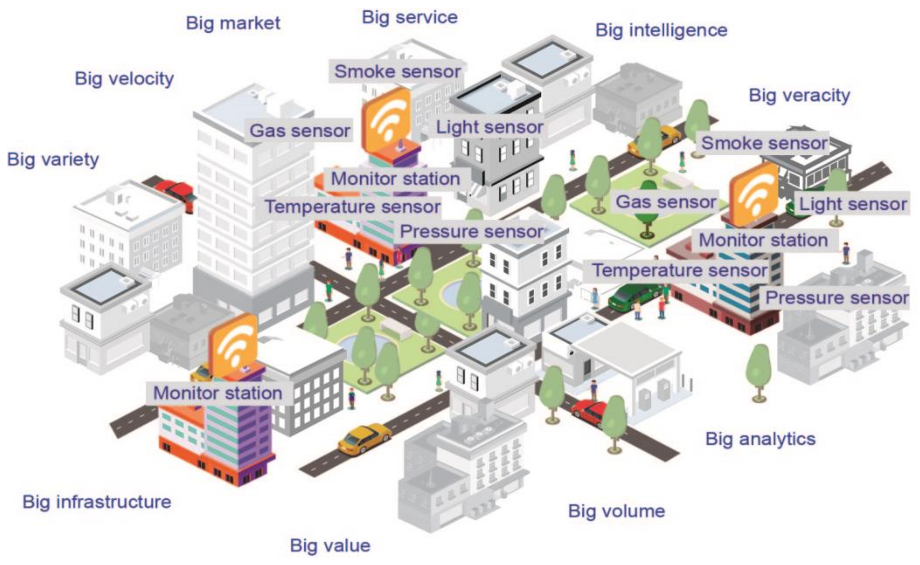
Big data deals with the management of high volumes of data, as well as their storage. Big data is characterized by 10 ‘bigs’. These ‘bigs’ are classified by three levels of characteristics: fundamental, technological, and socioeconomic. The fundamental level is integrated by four bigs: big volume, big velocity, big variety, and big veracity. The technological level is formed by three bigs: big intelligence, big analytics, and big infrastructure. And the level of socioeconomic characteristics has three bigs: big service, big value, and big market [5]. Data recollected by sensors in the analysis of smart cites require technological achievements, supporting the primary goal of bringing smart cities to the requirements of socioeconomic characteristics. Figure 1 represents the association of the 10 bigs in a smart city.
Sensors allow collecting data from a context, detecting and responding to signals, which can be measured and then converted into understandable data through designed and developed models. Sensors can be installed both indoors and outdoors. Regarding interiors, sensors are those set in the human body, which allow collecting information about peoples’ daily activities. They are usually acceleration sensors, widely used for their low cost and small size. The first works carried out for these devices focused primarily on the recognition of various modes of locomotion. Later, they were used in more complex activities such as sports, industry, gesture recognition, sign language recognition, and the human–computer interfaces (HCI) [6].
For exterior sensors, location is very relevant—they must be placed strategically in order to provide as accurate information as possible, in such a way that big data analysis can provide the identification of behavior patterns and the reduction of response times required for the smart cities.
However, it must be taken into account that, in the official information sites of quality measurement, data is not usually displayed in real-time—the update of the evaluation of events is not immediate. Sensor data is usually set to be taken over time intervals, which might lead to undetected changes. On the other hand, there is a lack of systems that face the continuous increase in the volume of catches and sensors, which support the monitoring of events of various kinds, and the readjustment of the infrastructure in sensor networks.
There is great interest in the installation of sensors in various areas of the city, human body, buildings, or houses, thus covering multiple scales. The tendency is to converge upon the Internet of Things (IoT), which is the construction of a dynamic network infrastructure capable of changing its configuration for better control of the flow of variables that circulate through a large number of interconnected sensors [7]. Thus, being able to extract patterns and relate phenomena to their causes within an environment such as a city constitutes a complex system [8].
The proliferation of sensors is increasing, and with this, the applications that perform a scientific analysis on their generated data, along with the use of different variables which, in one way or another, contribute to improving human wellbeing. Such is the case of the mobile systems, in which data comes from sensors installed inside them [9], or the systems that use sensors for environmental monitoring [10].
Also, a paradigm proposed in smart cities is the mobile crowd sensing (MCS), which focuses on using mobile integrated sensors to monitor multiple environmental phenomena, such as noise, air, or electromagnetic fields in the environment [11]. In this same topic, a system of pollution warning services was developed for smart cities [12], to notify the user of the concentration of pollution in the place where they are located, through mobile devices that measure the quality of the air. For example, a system based on crowdsourcing for mobile phones was developed to help car users to find the most appropriate places to park, in order to avoid problems of traffic congestion, air pollution, and social anxiety problems [8].
Another system of pollution warning services in smart cities was proposed to notify the user regarding the concentration of pollution, and about vehicles. In this case, mobile devices measure air quality [10]. In [11], an implementation of smart sensors was presented to monitor air quality where the tracking variables included dust particles (PM10), carbon monoxide (CO), carbon dioxide (CO2), noise level (dB), and ozone (O3), with the aim to keep people informed in real-time through the IoT.
In this context, machine learning and deep learning are two successful techniques both used for the classification of data as well as the identification of patterns. Another technology used in the same context is bio-inspired algorithms for the interpretation of information from the sensors. However, since big data faces the challenge of large volumes of information, several techniques are combined with it to provide proper solutions.
As mentioned, the constant use of sensors in smart cities led to the field of big data, which deals with processing and data analysis techniques. Within a broad set of techniques and methods for processing big data are the decision trees (DT) based on classifiers applied to large datasets [13]—DTs are also proposed to analyze large data sets for both numerical and mixed-type attributes. By processing all the objects of the training set without prior memory storage, this requires that the user define the parameters. It works by evaluating the training instances one by one incrementally, updating the DT with each revised case. With a small number of instances, the node is expanded faster than the expansion process of other algorithms. Furthermore, the instances used in the expansion of the node will be eliminated once the expansion is made avoiding in this way the storage of the training set in the memory.
In this context, in [14] was proposed the use of swarm search with accelerated particle swarm optimization. This is an algorithm capable of selecting the variables for data mining—its search achieves precision in a reasonable processing time. Further, in [15] was presented a system based on the ideas of pattern recognition that converges in the Bayes classifier. This system is scalable in data and can be implemented using structured query language (SQL) over arbitrary database tables—it uses disk storage with classification purposes. In [16], the algorithm C4.5 implemented a DT with the map-reduce model, to allow parallel computing of big data. This algorithm implements map-reduce with the ‘divide and conquer’ approach in order to discover the most relevant attributes of the data set for decision-making.
Importantly, neither of the two techniques using and not using discs for the training of big data ensure that there are defined patterns.
Related Work
In this paper, we propose a classification scheme based on machine learning, using big data generated to construct patterns in real-time for the fixed location of sensors. These patterns will provide the surrounding areas with a low quality of life in order to establish a better-fixed location for new sensors, or the relocation of the old sensors with the information generated by them through established hot-zones. Therefore, some related works regarding sensor locations are next discussed.
In [6] are presented different methodologies for selecting the places where the sensors should be installed to obtain information on the phenomena to be observed, ranging from the preparation of a grid of the study area to the use of complex statistical models that provide the number and optimal distribution of the sensors, but this is based strictly on the amount of information with which the model is generated.
In [17] is implemented a genetic algorithm (GA) to determine sensor locations and to establish the number of these sensors for proper coverage. As a first step, the GA randomly creates the population on the input map. This algorithm has the main feature of finding the number of optimum sensors based on the input map.
In [18] is presented an algorithm that simultaneously defines a sensor placement and a sensor scheduling. An approximation algorithm with a finite set of possible locations establishes where sensors can be placed; this algorithm selects a small subset of locations. These works focus on locating the sensors through random functions or by a set of defined positions.
There are several works related to the location of sensors for smart cities. Furthermore, some of them have a dynamic identification for sensors positions. However, few of them focus on the identification of fixed positions and, to our knowledge, none of them exploit the information acquired by the same sensors with big data techniques in order to identify their optimal location or relocation. In contrast, our proposal establishes the location of sensors in real-time using the concept of hot-zones in order to identify the sensors with significant activity regarding the phenomena observed with high precision.
We defined the concept of a ‘hot-zone’ as a perimeter area source of essential data for analysis. In a hot-zone can be found constant activity with substantial data to evaluate the quality of an observed phenomenon. These hot-zones are then used to locate or relocate new sensors. For that, a process with four phases is proposed. The first three phases are based on the data mining process, and the fourth phase constitutes the establishment of algorithms using selected techniques. The final aim of the process is to settle the hot-zones.
As an example, this process was implemented in the Guadalajara Metropolitan Zone (GMZ), Mexico, for air pollution. In this case, a first algorithm was designed for data training to generate the classification model with dynamic updating. A second algorithm was designed for data labeling, which is triggered after each data input. The two algorithms are independent. The classification is carried out in parallel with the training process—while some data are classified, others are used for training to observe possible changes in the patterns, or to decrease process time by a possible reduction in the number of variables of the model. In this phase, a frequency matrix is generated that works in conjunction with a neighboring sensor matrix in order to identify the hot-zones and present their visualization in a geo-referenced map [19,20].
2. Process to Locate and Relocate Sensors
Our proposed process comprises four phases:
- The preparation of sample data;
- The inquiry or exploration of data analysis methods for big data treatment;
- Exploring prediction techniques; and
- Algorithms design and updating of the map to locate and relocate sensors.
The process is based on the data mining process for knowledge discovery in data bases (KDD) ] [21] and which, according to [22], should be guided by the seven phases: data integration, data selection, data cleaning, data transformation, data mining, pattern evaluation/presentation, and knowledge discovery. Data mining is the step of selection through the application of machine learning techniques, in this case, aiming to find classification patterns for hot-zone identification.
Similarly, in our process, the first phase corresponds to data integration, data selection, data cleaning, and data transformation. In our case, it consists of reviewing the quality of life in smart city models in order to select variables according to the standards, and then extracting data from open data public domains to conform the data set. Afterward, the sample is prepared by applying a filter, cleaning, and when required labeling, which constitutes data cleaning and data transformation.
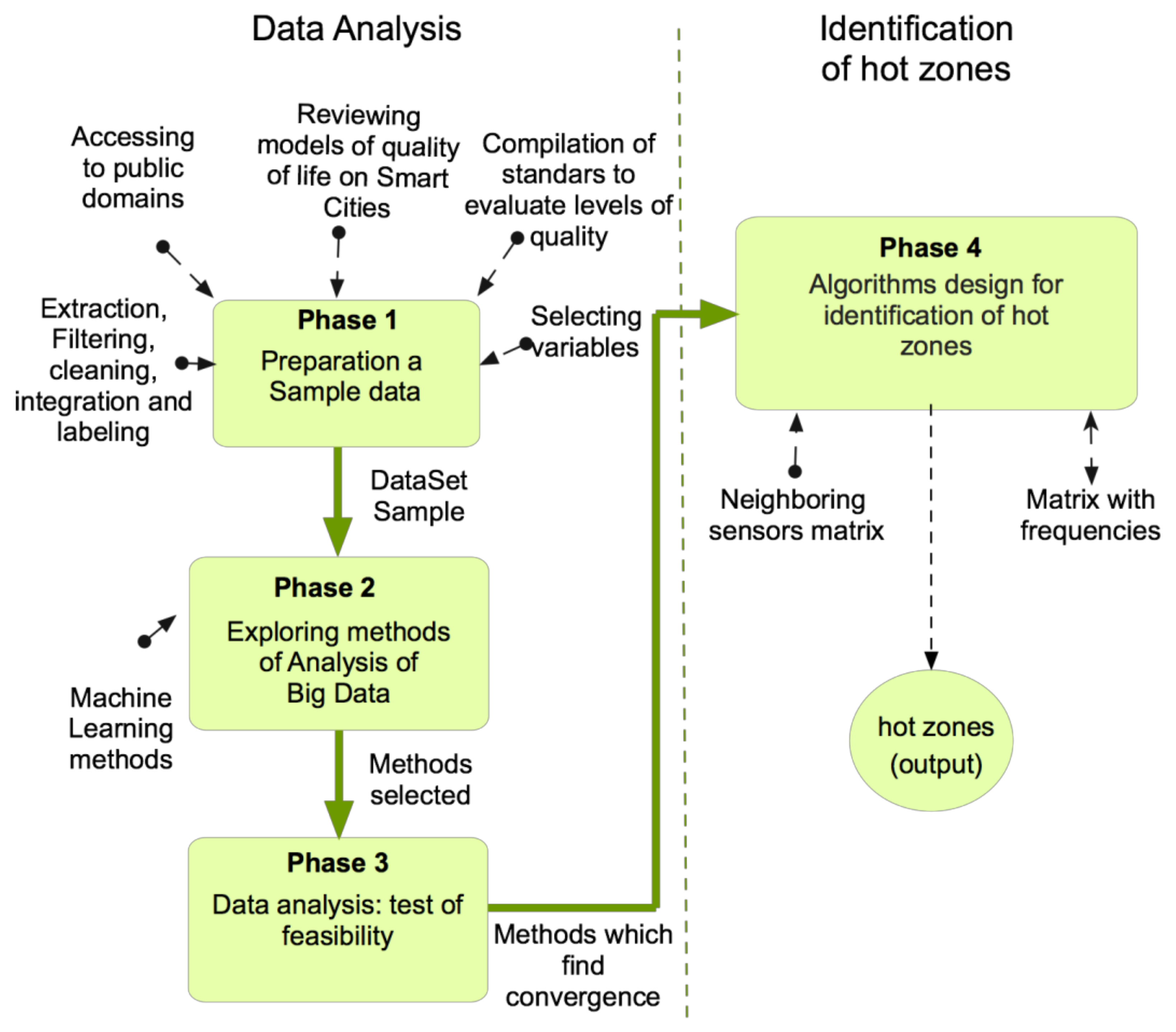
Figure 2 depicts the four phases. The first phase is the preparation of the data sample, which begins with the revision of the smart city models and the compilation of standards related to the object of study selected. These activities will indicate the variables that the sensors must capture but, at the same time, will guide the search of data in public domains to form a sample data set. Here, preprocessing for filtering and cleaning is also applied. The result to be obtained is a sample of data validated by the metrics of the smart city models, and by models established by international organizations.
Once the data is transformed, it goes to Phase 2 for big data analysis focused on data mining, optimizing the performance of the search of the classification patterns.
In the second phase, the exploration of data analysis is performed using supervised learning techniques for classification in order to arrive at a prediction model, using as input the sample of the data set of the previous phase. It is suggested to explore techniques with parallelization capacity in order to optimize the processing time of patterns from large volumes of data. Also, independent variables must be clearly distinguished from their dependent counterparts. The output of phase two is a candidate list of techniques to be tested in the Phase 3.
In the third phase, the selected techniques are tested with the prepared data sample. Here, a plan has to be made to test and apply the candidate techniques. Then, those whose convergence obtained is equal to or greater than the desired limit are chosen. Another factor that should influence this selection is the technique’s capacity to reduce variables. The convergence results are sent to the Phase 4, as the basis for the algorithm’s design.
In the fourth phase are designed and implemented the algorithms. Two types of algorithm are required for the identification of the hot-zones.
The first type of algorithm is those that apply the chosen techniques in Phase 3, that is, those with better convergence results. These algorithms serve for the extraction of data patterns from the model. The second algorithm type includes those that classify and update the frequency matrix with the neighboring sensor matrix shapes of the hot-zones.
The application of the algorithms implies the existence of a set of sensors in the network, where every installed sensor has a pair of values related to its geographical localization: latitude and longitude. Further, it also emits the value of variables. Although the sensor placement points are initially selected for a better control of the areas, it does not necessarily mean that they are located in the focus of the phenomenon, especially if there are not enough sensors, or if they are dispersed.
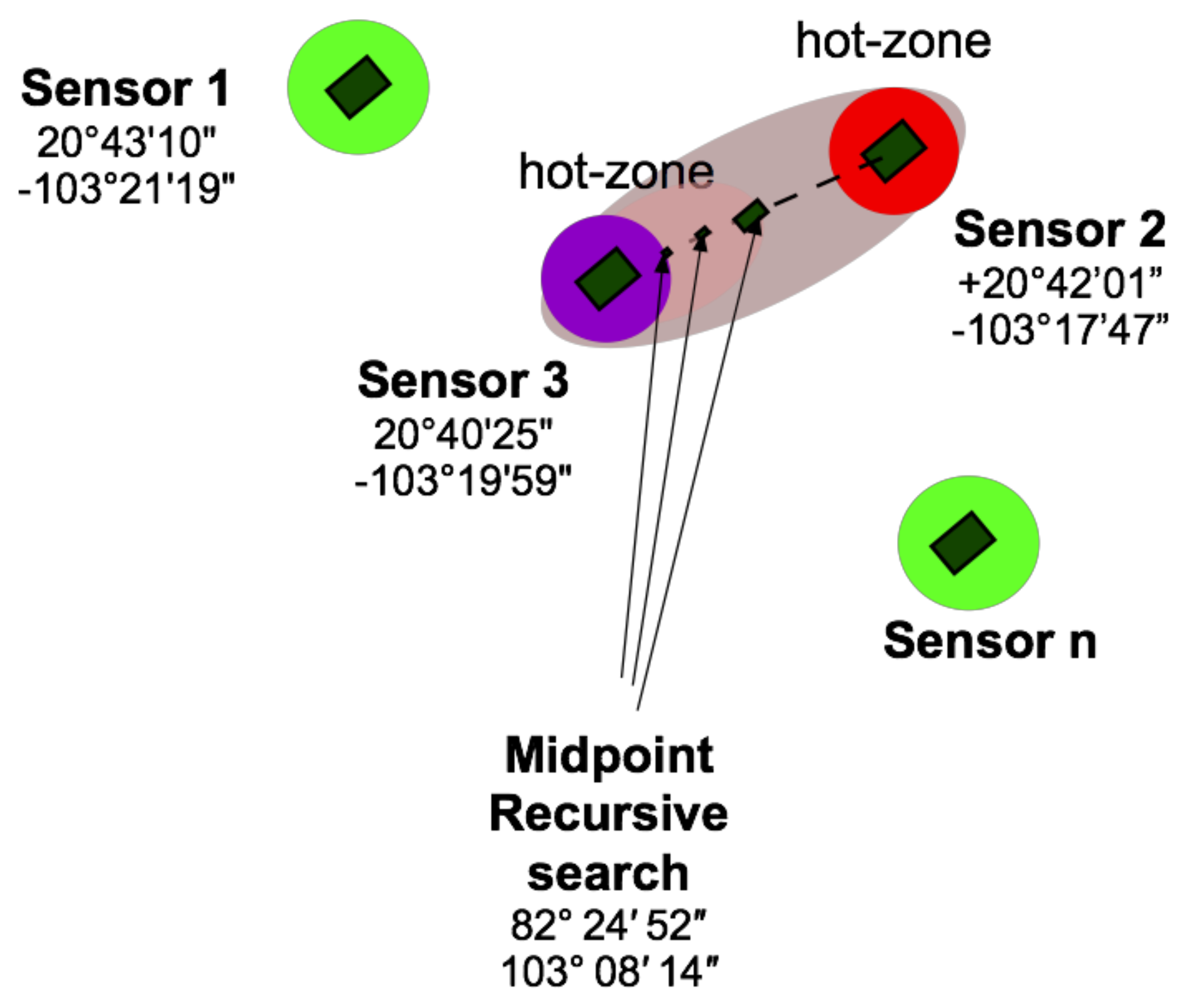
By recursively identifying the hot-zones, that is to say, applying or reapplying Phase 4 of the process, midpoints between two sensors can be inferred—this represents the proposed fixed locations to place a new sensor. With newly located sensors, we can get new and different matrices with a reduced scope of hot-zones.
In Figure 3, an example of dispersed sensors in a geo-referenced region is observed. Two of the four sensors were identified as hot-zones: Sensor 2 (in red) and Sensor 3 (in magenta) in contrast with green sensors. In Figure 3, the scope of the hot-zone is reduced, approaching sensor 3, but it could go to the other way around, approaching sensor 2. The scope of the hot-zone will be reduced based on the sensors’ data and using the analogy of a binary search, that is, taking one of two paths. This process will generate another dynamic map of the sensor.
In the next section, the process is applied for a specific situation.
3. Process Implementation
A critical problem in the big cities is air quality. Therefore, air pollution indicators of the Guadalajara Metropolitan Zone (GMZ) in the Jalisco State of Mexico were treated. The GMZ is the second most populous area in Mexico with more than 5 million habitants.
In order to choose our data sample, we consulted the official Mexican standards for population health [23,24], which recommended the following variables: PM10, PM2.5, O3, NO2, SO2, and carbon monoxide (CO) [23], and the World Health Organization (WHO) whose guidelines for improving air quality include the reduction of particulate matter (PM), ozone (O3), nitrogen dioxide (NO2), and sulfur dioxide (SO2).
For Phase 1 of the process (see Figure 2), we downloaded files from the information page of the Secretariat of the Environment and Territorial Development of Jalisco State [25], in Microsoft Office Excel software format. Data from 21 years of air variables, from 1996 to 2017, were recovered. Sensor data monitoring started with eight stations and, in 2012, two additional stations were added. The records contained data from every hour for each station. After analyzing the data, January to December, 2015 was selected as a sample. In this year, the 10 stations were implemented, and it presented fewer missing values when compared with other years.
For Phase 2 of the process, the dataset was cleaned—that is, null data were eliminated. Also, the variable PM2.5 was not considered because, initially, there were no sensors for it. Moreover, when sensors that could monitor it were installed, they contained a massive amount of null values.
Observations were labeled according to a certain level of air quality, as indicated by the Mexican reference Metropolitan Index of Air Quality (IMECA by its Spanish initials), as shown in Table 1.
The variables have a different range. The variable with the highest value according to its range is the one that indicates the air quality level by color. Pollution levels are classified as: good = level 1 in green color; fair = level 1 in yellow color; bad = level 5 in orange color; very bad = level 4 in red color, and extremely bad = level 5 in magenta color. Table 2 shows an extract of registered entries in a file after being classified with the quality label in the sixth column.
Then, data analysis algorithms were selected. As mentioned with the objective of discarding, if possible, some variables with less influence for the quality classification. Also, algorithms to train with machine learning that require fixed-size datasets and disk storage were selected, because it added a function of partial elimination of records in the cloud. For Phases 3 and 4, the R language, kernlab, e1071, rpart, and doParallel libraries were applied to support the process.
Three prediction methods were tested: multiple linear regression (MLR), support vector machine (SVM), and decision trees implementing a classification and regression tree (CART). The first one (MLR) was chosen to explore the linear model. The second and third methods were used for testing because of the advantages they present, such as parallelization and reliability.
For the MLR test, six variables were involved—the quality label as a dependent variable, and CO, NO2, O3, PM10, and SO2 as independent variables. Once the files were cleaned and filtered, 66,880 observations formed the data sample. The data-training group contained 70% of these observations, with a total of 46,816 observations. The MLR test presented an R-squared of 58.13%, not reaching the expected 80%, indicating that the data did not fit a linear function.
For the SVM, two groups were formed: the training and testing groups. The first group contained 46,816 records, and the testing group 20,064 records, the values for the kernel parameter were rbfdot, radial, and hyperparameter sigma = 0.5. For both, the training error of 20% was obtained. The equivalent algorithm for both cases is represented by a mathematical equation in which the outputs are the Quality level; this virtually eliminates comparisons and decreases execution time.
CART showed a root node error of 16974/66881 = 0.25379, reducing the comparison variables PM10 and O3. However, the model does not classify for level 5 because there are few entries with that label, so that specific output is not explained, as shown in Figure 4.
3.1. Algorithms for Classification and Training
The goal of these algorithms is to classify data and each data acquisition, from the sensor a set of variables is identified as a record=(_n 1){ variable _i }, where n is the given number of variables of instrumentation, for example, light intensity, humidity, or movement. To get the registration form as register = |1|2||3||n| where each number is associated with a risk level of quality, as indicated by the standards. In our case of study, the record is formed by the variables register = CO, NO2, O3, PM10, SO3 to be classified according to the level of quality from the IMECA index.
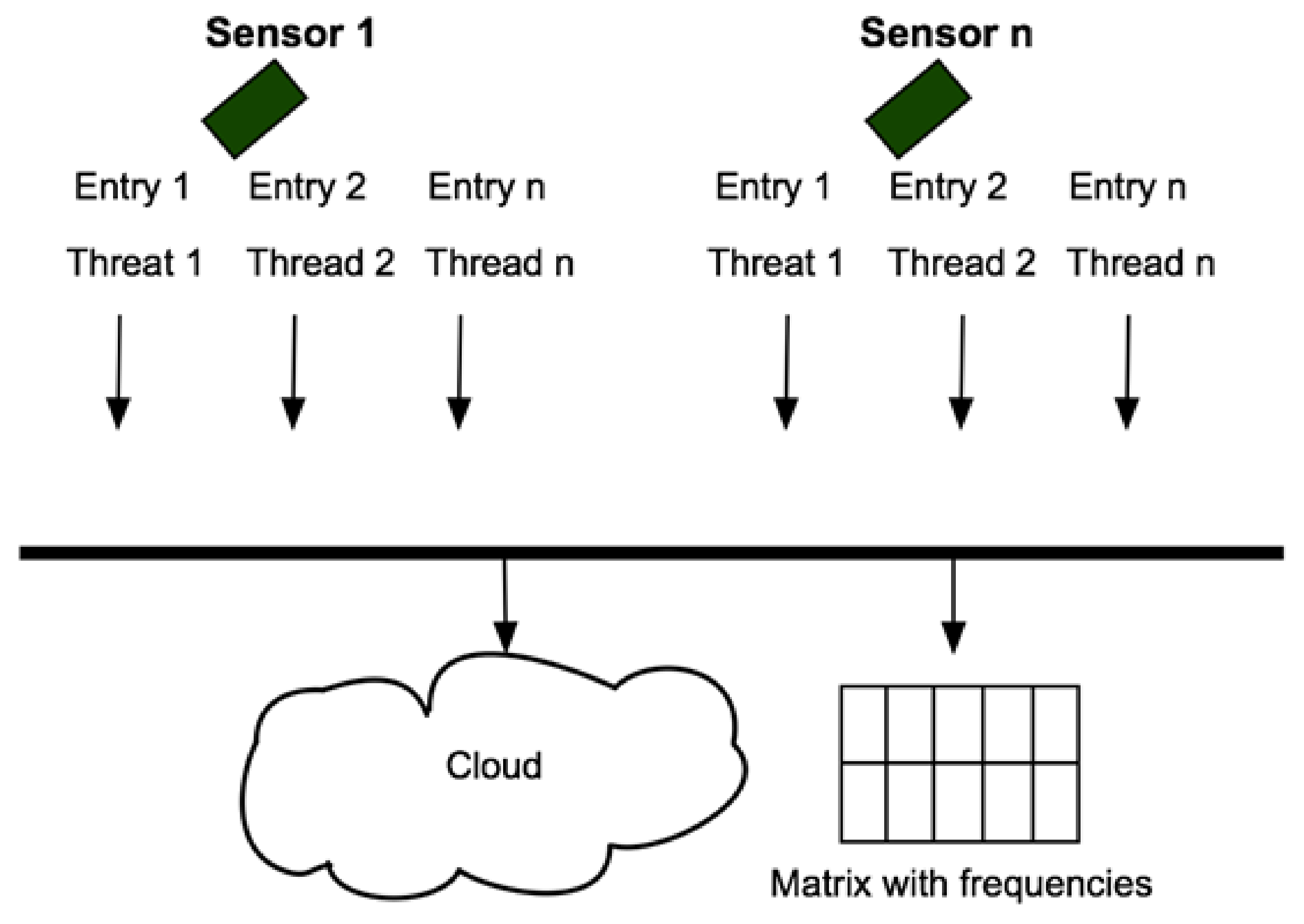
According to the results of Phase 3 of the process (see Figure 2), in Phase 4, the algorithms were executed—the algorithm to classify the sensor inputs, and the algorithm for training and setting the prediction model. Here, we proposed an architecture that allows each sensor to dispatch data captured to different processing threads, using cloud computing for a distributed performance, and with access to the shared memory. Figure 5 depicts the parallel processing of the data inputs captured by the sensors, their destinations in the cloud, and a matrix with frequencies, the shared memory variable to identify the hot-zones.
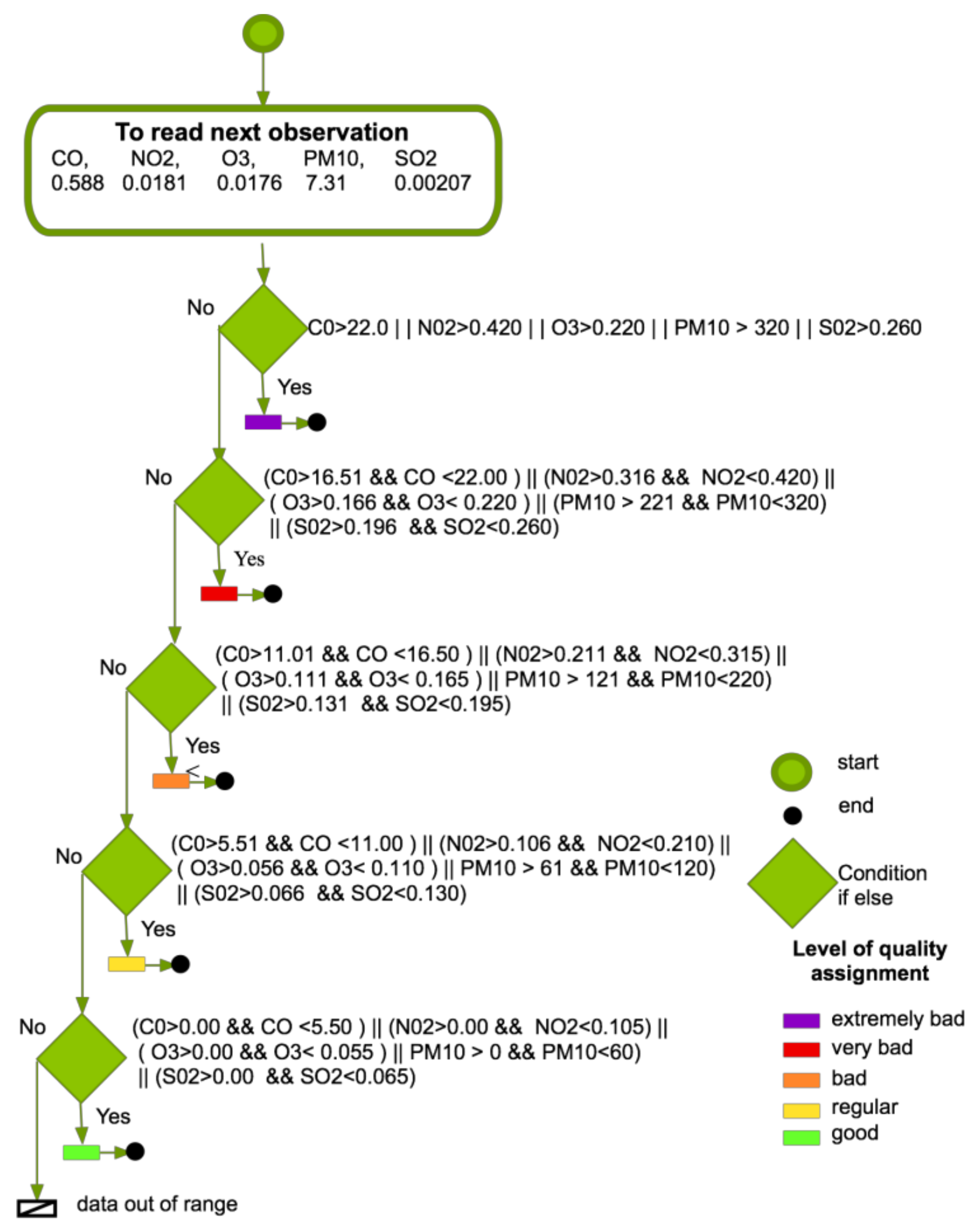
Classifying the sensor’s inputs can be made by a table in memory, in which the intervals for the variables are specified. In this case, a systematic review is carried out, starting with the values that exceed the limits in the IMECA classification. The best case is when just one comparison is needed, and the worst case is when the variable does not exceed any previous interval and must continue with the comparisons to the green level 1—see Figure 6.
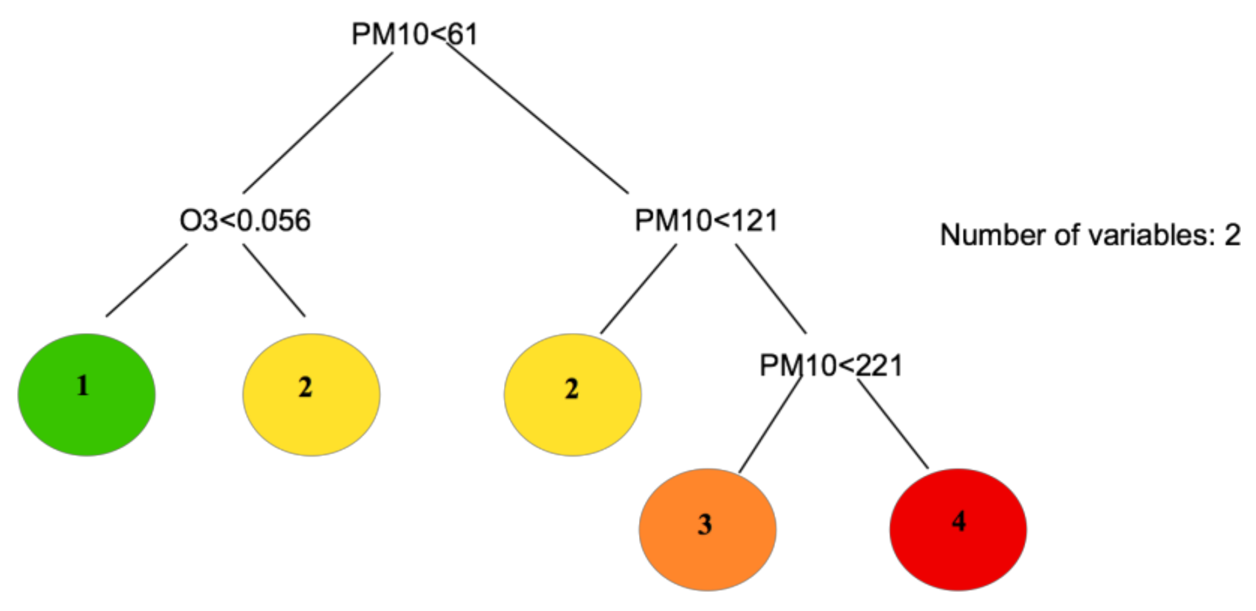
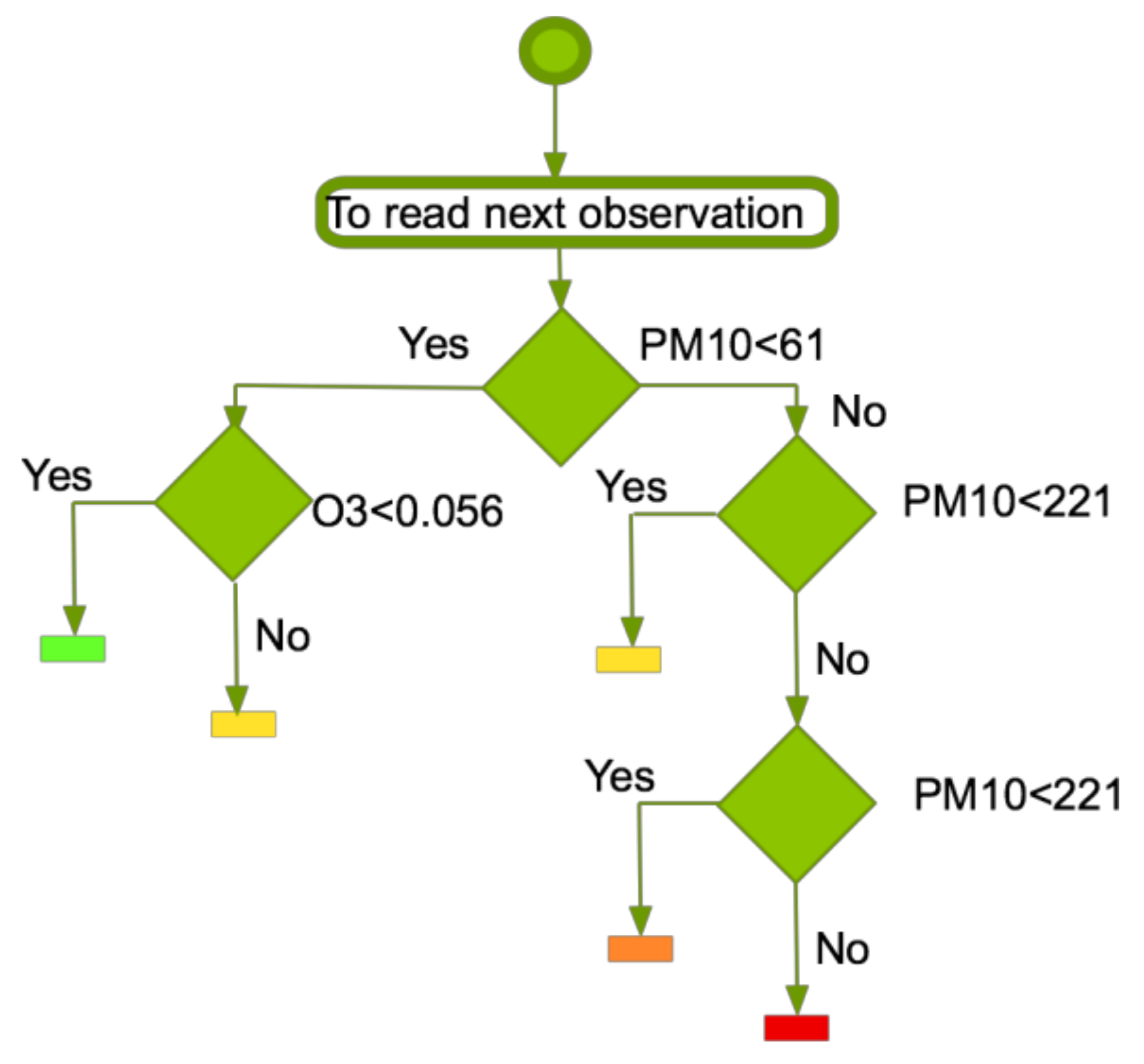
This classification can be optimized through CART reducing conditions, as can be observed in Figure 7. In this case, the number of variables is two (PM10 and O3)—the input lacks some variable values (i.e. CO, SO2, or NO2 variables) that are not necessary in this case for the classification.
It is essential to highlight that, if a mathematical model presents a proper classification solution, for example, through the MLR model, that must be the less resource-consuming path to follow. Otherwise, as in this case, a classification method has to be selected. In any case, a matrix with the frequencies of sensors’ events has to be updated. This update requires observing a time range. It is also necessary to label a representative sample of the big data burst, which will be used as a training group, maintaining the observation stored. The remaining registers are eliminated, avoiding the demand for storage space.
Cloud storage occurs to form a temporary dataset for training, to take advantage of resources, and to distribute tasks for the tests with machine learning techniques. In the cloud, a process is activated when a sample size or a specific period is reached. The process consists of using the training data with the selected methods in Phase 3 of the process. In this example, SVM and CART run in parallel and are distributed concurrently. The algorithm finally updates the classification model to be read by the threads that will perform the classification.
3.2. Matrices for the Dynamic Map
The objective of the frequency matrix is to provide an environment variable in shared memory. This variable content is the sum of incidents specifying time intervals with high risk. Frequent readings to this matrix will be performed to draw on a georeferenced map with the current sensors.
The frequency matrix accumulates the number of quality levels labeled (see Figure 5) during a specific time. In this way, the sensors with the highest levels of pollution are easily identified—Table 3 depicts one of these periods for five sensors. In Table 3, it can be observed that sensors 3, 4, and 5 have the highest frequency in Level 5, meaning that they are classified as extremely bad.
In order to locate or relocate sensors, a matrix indicating sensors in neighboring areas is required. See, for example, Table 3, where the name to identify the sensor implies its coordinates. In Table 4 can be observed, for instance, that Sensor 1 (Oblatos) in the first row is in the surrounding area with Sensors 2, 4, and 5 (Centro, Tlaquepaque, and Loma Dorada) indicated by a number ‘1’ in those columns.
Matching frequency matrix to the neighbor sensors with high pollution levels can be deduced. Locating new sensors in the highest levels of pollution will help getting a better understanding regarding the contamination source or the type variants that are affecting the area. The dynamic model might change the location requirements by distinguishing a new sensor’s location or the relocation of those that are already in the system.
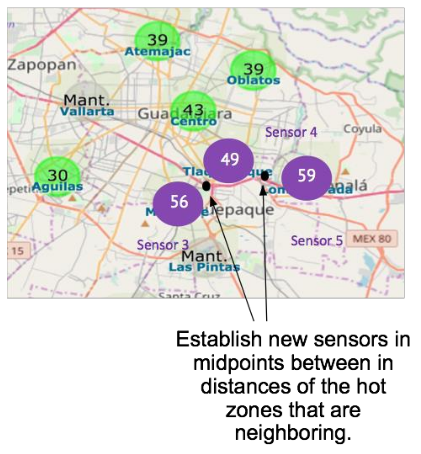
In our example, new sensors could be located where the two arrows point in Figure 8. These are between sensors 3 and 4, and sensors 4 and 5 (corresponding to Miravalle, Tlaquepaque and Loma Dorada). According to the frequency matrix in Table 3, these three sensors have a high number of records at level 5, or Extremely bad, and they also correspond to neighboring areas according to the neighboring matrix in Table 4, where it can be observed that sensor 3 is adjacent to sensor 4, and sensor 4 is adjacent to sensor 5.
4. Conclusions
The development of smart cities has led to the increase of sensors in cities—with them, it is possible to identify phenomena to meet one of its main objectives, the development of quality of life and sustainability. Therefore, it is essential to have methods that help to establish a better location for new sensors in existing critical points or hot-zones.
We propose that the analysis of the data generated by the same sensors, provides information helpful to identify the hot-zones, and to locate or relocate sensors.
Based on the data mining paradigm, we observed that this is not sufficient for a dynamic system. Thus, our process includes the last phase for the recognition and visualization of hot-zones, a perimeter with significant data related to the observed phenomenon. The information captured by the sensors determines the location of new sensors, or the relocation of those already receiving data.
The proposed process offers a scheme for data labeling, creating a dynamic classification model. The classification and training algorithms in the cloud manage an independent control. Then, prediction techniques required to be tested to get those that better fit the data.
In our case study, data regarding air pollution in the Guadalajara Metropolitan Zone in Mexico was analyzed and, for that, the SVM was selected. With the SVM, different parameters were tested, and it was adjusted to different kernels, allowing for more accurate predictions.
Finally, two algorithms were designed as a result of the application of the process. These algorithms are independent processes on threads using cloud computing. The first one classifies each one of the entries captured in order to generate a matrix of territorial adjacencies. The second one is trained with a classification and regression tree (CART) and SVM. Although the development of the algorithms was performed in the context of environmental variables, this proposal is autonomous with respect to the sensors’ features. It can also be scaled to various types, including the quantity and volume of information, because it does not require data storage. It is worth mentioning that it is necessary to continuously verify the local and international standards for the algorithms since new sensors might be incorporated varying in variables and ranges.
In future work, the combinations of variables obtained from sensors, along with other retrieving variables, such as those coming from questionnaires, social media, or government data, will be included.
Author Contributions
Conceptualizacion, E.E. and M.P.M.V.; Methodology A.P.P.N.; Software, E.E. and J.G.; Validation G.L.L.; Formal analysis E.E. and A.P.P.N.; Investigation, E.E., M.P.M.V., J.G., and R.M.; Data curation, E.E. and J.G., Writing—Original draft preparation E.E.; Writing—Review and editing E.E., A.P.P.N. and M.P.M.V.; Visualizacion M.P.M.V.; Supervision A.P.P.N.
Funding
This research received no external funding.
Acknowledgments
We would like to thank Marco Pérez-Cisneros director of the Electronic and Computer Division of the CUCEI for his support.
Conflicts of Interest
The authors declare no conflict of interest.
References
- Smart City Ventajas y Desventajas de las Ciudades Inteligentes. Available online: https://ovacen.com/smart-city-ventajas-y-desventajas/ (accessed on 9 June 2019).
- Martínez, Y. El 60% de la Población Mundial Vivirá en Ciudades en 2030. Revista Electrónica de Ciencia, Tecnología, Sociedad y Cultura. 2008. Available online: https://www.tendencias21.net/El-60-de-la-poblacion-mundial-vivira-en-ciudades-en-2030_a2715.html (accessed on 9 June 2019).
- Organización Mundial de la Salud. Available online: http://www.who.int/topics/air_pollution/es/ (accessed on 3 May 2019).
- Gómez, J.E. Modelado de Algoritmos y Análisis de Big Data para Determinar las Coordenadas de Instalación de Sensores en Áreas Territoriales de Mayores Niveles de Contaminación Atmosférica en la ZMG. Master’s Thesis, Universidad de Guadalajara, Guadalajara, Mexico, 2019. [Google Scholar]
- Sun, Z. 10 Bigs: Big Data and Its Ten Big Characteristics. PNG Univ. Technol. 2018, 3, 1–10. [Google Scholar] [CrossRef]
- Martínez, A.P.; Romieu, I. Introducción al Monitoreo Atmosférico; ECO: Guadalajara, Mexico, 1997. [Google Scholar]
- González, V.H. Tutorial: Internet of Things and the upcoming wireless sensor networks related with the use of big data in mapping services; issues of smart cities. In Proceedings of the 2016 Third International Conference on eDemocracy & eGovernment (ICEDEG), Sangolqui, Ecuador, 30 March–1 April 2016; pp. 5–6. [Google Scholar]
- Duangsuwan, S.; Takarn, A.; Nujankaew, R.; Jamjareegulgarn, P. A Study of Air Pollution Smart Sensors LPWAN via NB-IoT for Thailand Smart Cities 4.0. In Proceedings of the 2018 10th International Conference on Knowledge and Smart Technology (KST), Chiang Mai, Thailand, 31 January–3 February 2018; pp. 206–209. [Google Scholar]
- Mitsopoulou, E.; Kalogeraki, V. Efficient Parking Allocation for SmartCities. In Proceedings of the PETRA ‘17 10th International Conference on PErvasive Technologies Related to Assistive Environments, Island of Rhodes, Greece, 21–23 June 2017; pp. 265–268. [Google Scholar]
- Osama, A.; Ghoneim, D.B. Forecasting of Ozone Concentration in Smart City using Deep Learning. In Proceedings of the IEEE 2017 International Conference on Advances in Computing, Communications and Informatics (ICACCI), Udupi, India, 13–16 September 2017; pp. 1320–1326. [Google Scholar]
- Longo, A.; Zappatore, M.; Bochicchio, M.; Navathe, S.B. Crowd-Sourced Data Collection for Urban Monitoring via Mobile Sensors. ACM Trans. Internet Technol. 2017, 18, 5. [Google Scholar] [CrossRef]
- Rodríguez, S.; Walter, S.; Pang, S.; Deva, B.; Küpper, A. Urban Air Pollution Alert Service for Smart Cities. In Proceedings of the 8th International Conference on the Internet of Things, Santa Barbara, CA, USA, 15–18 October 2018. [Google Scholar]
- Franco, A.; Carrasco, J.A.; Sánchez, G.; Martínez, J.F. Decision Tree based Classifiers for Large Datasets. Comput. Sist. 2013, 17, 95–102. [Google Scholar]
- Fong, S.; Wong, R.; Vasilakos, A.V. Accelerated PSO Swarm Search Feature Selection for Data Stream Mining Big Data. IEEE Trans. Serv. Comput. 2016, 9, 33–45. [Google Scholar] [CrossRef]
- Mortonios, K. Database Implementation of a Model-Free Classifier. In Advances in Databases and Information Systems; Springer: Berlin/Heidelberg, Germany, 2007; Volume 4690, pp. 83–97. [Google Scholar]
- Koli, A.; Shinde, S. Parallel decision tree with map reduce model for big data analytics. In Proceedings of the 2017 International Conference on Trends in Electronics and Informatics (ICEI), Tirunelveli, India, 11–12 May 2017; pp. 735–739. [Google Scholar]
- Robatmili, M.; Mohammadi, M.; Movaghar, A.; Dehghan, M. Finding the sensors location and the number of sensors in sensor networks with a genetic algorithm. In Proceedings of the 2008 16th IEEE International Conference on Networks, New Delhi, India, 12–14 December 2008; pp. 1–3. [Google Scholar]
- Krause, A.; Rajagopal, R.; Gupta, A.; Guestrin, C. Simultaneous placement and scheduling of sensors. In Proceedings of the 2009 International Conference on Information Processing in Sensor Networks, San Francisco, CA, USA, 13–16 April 2009; pp. 181–192. [Google Scholar]
- Garcia, M.; Morales, J.; Menno, K. Integration and Exploitation of Sensor Data in Smart Cities through Event-Driven Applications. Sensors 2019, 19, 1372. [Google Scholar] [CrossRef]
- Estrada, E.; Maciel, R.; Peña, A.; Lara, G.; Larios, V.; Ochoa, A. Framework for the Analysis of Smart Cities Models. In Proceedings of the 7th International Conference on Software Process Improvement (CIMPS 2018), Guadalajara, Mexico, 17–19 September 2018. [Google Scholar]
- Fayyad, U.; Piatetsky-Shapiro, G.; Smyth, P. Knowledge Discovery and Data Mining; Towards a Unifying Framework. In Proceedings of the Second International Conference on Knowledge Discovery and Data Mining, Portland, OR, USA, 2–4 August 1996; pp. 82–88. [Google Scholar]
- Sumiran, K. An Overview of Data Mining Techniques and Their Application in Industrial Engineering. Asian J. Appl. Sci. Technol. 2018, 2, 947–953. [Google Scholar]
- Gaceta Oficial del Distrito Federal. Norma Ambiental para el Distrito Federal NADF-009-AIRE-2006. 2006. Available online: http://siga.jalisco.gob.mx/assets/documentos/normatividad/nadf-009-aire-2006.pdf (accessed on 9 June 2019).
- Diario Oficial de la Federación Mexicana. Norma Oficial Mexicana Nom-020-SSA1-2014, Salud Ambiental. Valor Límite Permisible para la Concentración De Ozono (O3) en el Aire Ambiente y Criterios para su Evaluación. 2014. Available online: http://www.aire.cdmx.gob.mx/descargas/monitoreo/normatividad/NOM-020-SSA1-2014.pdf (accessed on 9 June 2019).
- Secretaría de Medio Ambiente y Desarrollo Territorial. Available online: http://siga.jalisco.gob.mx/aire2018/mapag2019 (accessed on 9 June 2019).
Figure 1.
Sensors monitoring events on a Smart City from a perspective of Big Data as 10 bigs.

Figure 2.
Phases of the proposed process that determine a scheme to design algorithms to place sensors in specific positions.
Figure 2.
Phases of the proposed process that determine a scheme to design algorithms to place sensors in specific positions.

Figure 3.
A recursive search of midpoints within hot-zones.

Figure 4.
Training results using machine learning applying the CART classification technique.

Figure 5.
A general scheme of big data analysis with classification threads, an updated matrix with frequencies of pollution levels, and cloud training.
Figure 5.
A general scheme of big data analysis with classification threads, an updated matrix with frequencies of pollution levels, and cloud training.

Figure 6.
Flowchart for level classification.

Figure 7.
CART Algorithm from data training.

Figure 8.
Georeferenced map the neighbor’s sensor border on a first run of a recursive process.


Table 1.
Concentration intervals for color assignment or air quality levels [24].
Table 1.
Concentration intervals for color assignment or air quality levels [24].
| IMECA | O3 [ppm] | NO2 [ppm] | SO2 [ppm] | CO [ppm] | PM10 [mg/m3] |
|---|---|---|---|---|---|
| 0–50 | 0.000–0.055 | 0.000–0.105 | 0.000–0.065 | 0.00–5.50 | 0–60 |
| 51–100 | 0.056–0.110 | 0.106–0.210 | 0.066–0.130 | 5.51–11.00 | 61–120 |
| 101–150 | 0.111–0.165 | 0.211–0.315 | 0.131–0.195 | 11.01–16.50 | 121–220 |
| 151–200 | 0.166–0.220 | 0.316–0.420 | 0.196–0.260 | 16.51–22.00 | 221–320 |
| >200 | >0.220 | >0.420 | >0.260 | >22.00 | >320 |
Table 2.
Fragment of the sample of observations captured by sensors classified with a quality label.
Table 2.
Fragment of the sample of observations captured by sensors classified with a quality label.
| CO | NO2 | O3 | PM10 | SO2 | Quality |
|---|---|---|---|---|---|
| 0.588 | 0.0181 | 0.0176 | 7.31 | 0.00207 | 1 |
| 1.139 | 0.02767 | 0.01062 | 14.6 | 0.00197 | 1 |
| 2.235 | 0.03053 | 0.00178 | 65.8 | 0.00232 | 2 |
| 1.204 | 0.03698 | 0.01597 | 123.4 | 0.002 | 3 |
| 1.361 | 0.03257 | 0.0149 | 154.18 | 0.002 | 3 |
| 0.64 | 0.01578 | 0.00308 | 58.8 | 0.001 | 1 |
| 22.83 | 0.01503 | 0.00217 | 49.1 | 0.001 | 5 |
Table 3.
The frequency matrix of Quality levels with five sensors.
| Sensor | Level Quality 1 (Good) | Level Quality 2 (Fair) | Level Quality 3 (Bad) | Level Quality 4 (Very Bad) | Level Quality 5 (Extremely Bad) |
|---|---|---|---|---|---|
| 1 | 452,567 | 6,298,653 | 7,302,451 | 3,245,121 | 1,012,563 |
| 2 | 452,567 | 543,765 | 983,432 | 393,592 | 754,832 |
| 3 | 1,902,345 | 4,210,213 | 4,329,034 | 3,290,546 | 7,554,901 |
| 4 | 761,432 | 845,789 | 904,786 | 653,903 | 4,942,104 |
| 5 | 3,902,432 | 4,897,902 | 2,304,602 | 1,906,341 | 9,435,890 |
Table 4.
Neighboring sensors matrix.
| Sensor | Sensor 1 Oblatos | Sensor 2 Centro | Sensor 3 Miravalle | Sensor 4 Tlaquepaque | Sensor 5 Loma Dorada |
|---|---|---|---|---|---|
| 1 | 1 | 1 | 1 | ||
| 2 | 1 | 1 | 1 | ||
| 3 | 1 | 1 | |||
| 4 | 1 | 1 | |||
| 5 | 1 | 1 | 1 |
© 2019 by the authors. Licensee MDPI, Basel, Switzerland. This article is an open access article distributed under the terms and conditions of the Creative Commons Attribution (CC BY) license (http://creativecommons.org/licenses/by/4.0/).
Share and Cite
MDPI and ACS Style
Estrada, E.; Martínez Vargas, M.P.; Gómez, J.; Peña Pérez Negron, A.; López, G.L.; Maciel, R. Smart Cities Big Data Algorithms for Sensors Location. Appl. Sci. 2019, 9, 4196. https://0-doi-org.brum.beds.ac.uk/10.3390/app9194196
AMA Style
Estrada E, Martínez Vargas MP, Gómez J, Peña Pérez Negron A, López GL, Maciel R. Smart Cities Big Data Algorithms for Sensors Location. Applied Sciences. 2019; 9(19):4196. https://0-doi-org.brum.beds.ac.uk/10.3390/app9194196
Chicago/Turabian StyleEstrada, Elsa, Martha Patricia Martínez Vargas, Judith Gómez, Adriana Peña Pérez Negron, Graciela Lara López, and Rocío Maciel. 2019. "Smart Cities Big Data Algorithms for Sensors Location" Applied Sciences 9, no. 19: 4196. https://0-doi-org.brum.beds.ac.uk/10.3390/app9194196
Note that from the first issue of 2016, this journal uses article numbers instead of page numbers. See further details here.