Dynamics and Switching Control of a Class of Underactuated Mechanical Systems with Variant Constraints

Abstract

Locomotion systems with variant constraints are familiar in real world applications, but the dynamics and control issues of variant constraint systems have not been sufficiently discussed to date. From the viewpoint of Lagrange–d’Alembert equations with additional variable constraints, this paper investigates the modeling approaches of a class of hybrid dynamical systems (HDS) with instantaneously variant constraints and the switching control techniques of stabilizing the HDS to given periodic orbits. It is shown that under certain conditions there possibly exist zero impact periodic orbits in the HDS, and the HDS can be stabilized to the period-one orbits by a linear controller with only partial state feedback, even though the HDS are generally underactuated nonholonomic systems. As an example, a one-legged planar hopping robot is employed to demonstrate the main results of modeling and control of a class of HDS.

1. Introduction

Variant constraint systems, such as structurally reconfigurable systems, soft body locomotion systems, and contact or collision systems and so on, are familiar in real world applications. The variant constraint systems (VCS) are generally heterogeneous multi-mode systems and contain state jumps in the dynamics of the systems. Thus, the VCS is essentially a class of hybrid dynamical systems (HDS) [1,2].

Although the investigations about the HDS have been ongoing for more than thirty years [3], the dynamics modeling of general HDS has not been thoroughly discussed so far. For the VCS, a reasonable model can be used to analyze the dynamical behaviors of the systems, which can provide useful information for improving the mechanisms/structure designs and simultaneously reducing the complexity of synthesizing the control laws. Unfortunately, to date, a systemic approach of modeling the general VCS has not been presented. As shown in [1], many examples of HDS were presented, but the issues of modeling hybrid systems were discussed case by case. Hyon and Emura [4] briefly presented the modeling approach of the hybrid dynamics of a passive one-legged running robot, and did not mention the theoretical basis of the approach. In a monograph [5], Sadati et al. introduced the impact model of several kinds of dynamical legged robots in brief and the main contents of the monograph are motion planning and hybrid control issues of the HDS. In literature [6,7], Hurmuzlu et al. addressed the modeling and control approaches of the HDS with the background of the biped robots. Following the modeling approach presented by Hurmuzlu [6], Grizzle et al. [8,9] stablized the HDS of biped robots with the finite time controllers. From a viewpoint of nonlinear control [10], the VCS are generally a certain kind of nonholonomic system since a VCS usually has relatively fewer constraints in one mode while has more constraints in another mode, and the additional constraints themselves are possible nonholonomic constraints [11]. Brockett’s necessary condition [12] points out that the nonholonomic systems can not be stabilized by any smooth time invariant pure state feedback; thereafter, the presented controllers for nonholonomic systems commonly employ non-smooth feedback [11,13,14,15] or time varying feedback [11,16,17,18]. However, it is interesting that many theoretical or experimental investigations, such as the legged running robot systems [4,5,9], have shown that the underactuated nonholonomic systems [19] could be stabilized to certain time varying trajectories by switched linear controllers. The switched linear controllers [20] are a class of discontinuous controllers that do not violate the Brockett’s necessary condition. Therefore, as it is revealed in this paper, from a standpoint of switching control, under certain conditions, the complex VCS can be stabilized to certain periodic orbits by simple switched linear controllers with only partial state feedback in a time-sharing manner. This point is appealing in practice and supports the innovations of the VCS in a broader field well.

The remainder of this paper is organized as follows. In Section 2, modeling the hybrid dynamics of underactuated systems with variant constraints is discussed. It is shown that the impulse caused by the instantaneously variant constraints of the HDS can be explicitly calculated with the help of the concept of differential inclusions [21], so that searching for a time varying trajectory with zero impulse is possible, and the special time varying trajectory can be utilized to improve the energy efficient of a locomotion system. In Section 3, the switched linear control approaches for stabilizing the VCS are proposed. We show that the closed-loop stability of tracking trajectory for the HDS can be systematically investigated under the frame of switching control [22]. The benefits from the frame of switching control at least include that the relationship between the closed-loop stability and the characteristics of the subsystems in HDS can be analyzed in depth [23], and the substantial foundation of the switching control theory can provide good support for developing the relevant techniques of the HDS. In Section 4, as an example, the modeling, motion planning and stable hopping control of one-legged hopping robots are discussed in detail. Finally, in Section 5, the conclusions of this paper are presented.

2. Hybrid Dynamics of Underactuated Systems with Variant Constraints

This paper investigates the following system given by the Lagrange–d’Alembert equations [11,24]

$$\begin{array}{c}\hfill \frac{\mathrm{d}}{\mathrm{d}t}\frac{\partial L\left(\mathbf{q}\right)}{\partial \dot{\mathbf{q}}}-\frac{\partial L\left(\mathbf{q}\right)}{\partial \mathbf{q}}=\mathbf{W}\left(\mathbf{q}\right)\mathit{\lambda }+\mathbf{Bu},\end{array}$$

(1)

where $L(\mathbf{q},\dot{\mathbf{q}})=T(\mathbf{q},\dot{\mathbf{q}})-V\left(\mathbf{q}\right)$ is the Lagrangian, $T(\mathbf{q},\dot{\mathbf{q}})$ is the kinetic energy, $V\left(\mathbf{q}\right)$ is the potential energy of the system, $\mathbf{q}\in {\Re }^n$ is the generalized coordinates, $\mathit{\lambda }\in {\Re }^m$ is a vector of Lagrange multipliers, $\mathbf{W}\left(\mathbf{q}\right)\in {\Re }^{n\times m}$ is a functional matrix, $\mathbf{B}\in {\Re }^{n\times s}$ is the input matrix, and $\mathbf{u}\in {\Re }^s$ is the control input of the system. The term $\mathbf{W}\left(\mathbf{q}\right)\mathit{\lambda }$ in the right side of Equation (1) denotes the generalized forces caused by external constraints, which are usually introduced by certain interaction between the mechanical systems and the external environment, such as sliding, rolling, elastic or inelastic collision and so on, thus the external constraints are variable. Under the case $\mathbf{W}\left(\mathbf{q}\right)\mathit{\lambda }=0$, the corresponding system (1) is called under the least constraint mode. Otherwise, for the case $\mathbf{W}\left(\mathbf{q}\right)\mathit{\lambda }\ne 0$, the system is called under the full constraint mode. When $\mathbf{W}\left(\mathbf{q}\right)\mathit{\lambda }\ne 0$, as that systematically discussed in [11,24], there necessarily exist m constraint equations

$$\begin{array}{c}\hfill {\mathbf{W}}^{\mathrm{T}}\left(\mathbf{q}\right)\dot{\mathbf{q}}=0.\end{array}$$

(2)

If the constraint Equation (2) is integrable, then there exist m algebra equations $\mathbf{h}\left(\mathbf{q}\right)={(h_1,h_2,\dots ,h_m)}^{\mathrm{T}}=0$ that satisfy

$$\begin{array}{c}\hfill \mathbf{W}{\left(\mathbf{q}\right)}^{\mathrm{T}}=\frac{\partial \mathbf{h}\left(\mathbf{q}\right)}{\partial \mathbf{q}}.\end{array}$$

(3)

Then, system (1) is called a holonomic system. Otherwise, system (1) is a nonholonomic system if the differential constraints Equation (2) are non-integrable.

In order to analyze the state jumps before and after the constraint variation, define $t_{vc}^{+}$ and $t_{vc}^{-}$ to be the time just after and just before the constraint variations, respectively, $\mathsf{\Delta }{t}_{vc}=t_{vc}^{+}-t_{vc}^{-}$ is the interval of constraint variation, and define

$$\begin{array}{c}\hfill \tilde{\mathit{\lambda }}={\int }_{t_{vc}^{-}}^{t_{vc}^{+}}\mathit{\lambda }\mathrm{d}t\end{array}$$

(4)

to be the vector of the impulse caused by the constraint variation. In this paper, it is also supposed that the constraint variation is instantaneously completed, that is, $\mathsf{\Delta }{t}_{vc}\approx 0$, and

$$\begin{array}{c}\hfill \mathrm{d}\mathbf{q}\left(t\right)/\phantom{\mathrm{d}\mathbf{q}\left(t\right)\mathrm{d}t}\mathrm{d}t\in F(t,\mathbf{q}\left(t\right)),\left|F(t,\mathbf{q}(t\left)\right)\right|\le \delta \end{array}$$

(5)

for all $t\in \left[\begin{array}{cc}{t}_{vc}^{-}& t_{vc}^{+}\end{array}\right]$, where $\delta \ge 0$ is a positive constant, $\mathrm{d}\mathbf{q}\left(t\right)/\phantom{\mathrm{d}\mathbf{q}\left(t\right)\mathrm{d}t}\mathrm{d}t\in F(t,\mathbf{q}(t\left)\right)$ is called the differential inclusions [21]. According to the existence theorem of solutions of discontinuous systems (referring to Theorem 1, chapter 2 of [21]), the solution $\mathbf{q}\left(t\right)$ of the differential inclusions Equation (5) is absolutely continuous, that is, at the instant $t_{vc}^{}$, the coordinate variables $\mathbf{q}\left(t_{vc}^{}\right)$ do not change

$$\begin{array}{c}\hfill \mathbf{q}\left(t_{vc}^{+}\right)=\mathbf{q}\left(t_{vc}^{-}\right)\mathrm{for}\mathrm{all}t\in \left[\begin{array}{cc}{t}_{vc}^{-}& t_{vc}^{+}\end{array}\right].\end{array}$$

(6)

For system (1) with the variant constraints Equation (2), the impulse Equation (4) can be analytically calculated due to the following result.

Theorem 1. 

(Impulse calculation for general systems with variant constraints)

For system (1) with variant external constraints Equation (2), if $\mathsf{\Delta }{t}_{vc}\approx 0$, then the impulse Equation (4) caused by the constraint variation is explicitly given as

$$\begin{array}{c}\hfill \tilde{\mathit{\lambda }}=-{\left[{\mathbf{W}}^{\mathrm{T}}\left(\mathbf{q}\right){\mathbf{M}}_{}^{-1}\mathbf{W}\left(\mathbf{q}\right)\right]}^{-1}{\mathbf{W}}^{\mathrm{T}}\left(\mathbf{q}\right)\dot{\mathbf{q}}\left(t_{vc}^{-}\right)\end{array}$$

(7)

for adding constraints, and

$$\begin{array}{c}\hfill \tilde{\mathit{\lambda }}={\left[{\mathbf{W}}^{\mathrm{T}}\left(\mathbf{q}\right){\mathbf{M}}_{}^{-1}\mathbf{W}\left(\mathbf{q}\right)\right]}^{-1}{\mathbf{W}}^{\mathrm{T}}\left(\mathbf{q}\right)\dot{\mathbf{q}}\left(t_{vc}^{+}\right)\end{array}$$

(8)

for reducing constraints.

Proof. 

It is intuition that the following equation is satisfied:

$$\begin{array}{c}\hfill \frac{\partial V\left(\mathbf{q}\right)}{\partial \dot{\mathbf{q}}}=0.\end{array}$$

(9)

In addition, considering assumption Equation (5) and using condition Equation (6), we can conclude that

$$\begin{array}{c}\hfill \frac{\partial L(\mathbf{q},\dot{\mathbf{q}})}{\partial \mathbf{q}}=0\mathrm{and}\frac{\partial \mathbf{W}\left(\mathbf{q}\right)}{\partial \mathbf{q}}=0\end{array}$$

(10)

for all $t\in \mathsf{\Delta }{t}_{vc}$ since the Lagrangian $L\left(\mathbf{q}\right)$ and the constraints $\mathbf{W}\left(\mathbf{q}\right)$ are invariant during the instant $t\in \mathsf{\Delta }{t}_{vc}$. By integrating system (1) on every interval $\mathsf{\Delta }{t}_{vc}$ [6,7], we have

$$\begin{array}{c}\hfill \mathbf{M}·\mathsf{\Delta }\dot{\mathbf{q}}=\mathbf{W}\left(\mathbf{q}\right)\tilde{\mathit{\lambda }},\end{array}$$

(11)

where

$$\begin{array}{c}\hfill \mathsf{\Delta }\dot{\mathbf{q}}=\dot{\mathbf{q}}\left(t_{vc}^{+}\right)-\dot{\mathbf{q}}\left(t_{vc}^{-}\right).\end{array}$$

(12)

Combining with Equations (11) and (12), it follows that

$$\begin{array}{c}\hfill \dot{\mathbf{q}}\left(t_{vc}^{+}\right)-\dot{\mathbf{q}}\left(t_{vc}^{-}\right)={\mathbf{M}}_{}^{-1}\mathbf{W}\left(\mathbf{q}\right)\tilde{\mathit{\lambda }}.\end{array}$$

(13)

From Equation (2), we have

$$\begin{array}{c}\hfill {\mathbf{W}}^{\mathrm{T}}\left(\mathbf{q}\right)\dot{\mathbf{q}}\left(t_{vc}^{+}\right)=0\end{array}$$

(14)

for adding constraints, and

$$\begin{array}{c}\hfill {\mathbf{W}}^{\mathrm{T}}\left(\mathbf{q}\right)\dot{\mathbf{q}}\left(t_{vc}^{-}\right)=0\end{array}$$

(15)

for reducing constraints.

Substituting Equation (13) into Equation (14), it follows that

$$\begin{array}{c}\hfill {\mathbf{W}}^{\mathrm{T}}\left(\mathbf{q}\right)\dot{\mathbf{q}}\left(t_{vc}^{-}\right)+{\mathbf{W}}^{\mathrm{T}}\left(\mathbf{q}\right){\mathbf{M}}_{}^{-1}\mathbf{W}\left(\mathbf{q}\right)\tilde{\mathit{\lambda }}=0.\end{array}$$

(16)

Then, Equation (7) can be obtained. Substituting Equation (13) into Equation (15), it follows that

$$\begin{array}{c}\hfill {\mathbf{W}}^{\mathrm{T}}\left(\mathbf{q}\right)\dot{\mathbf{q}}\left(t_{vc}^{+}\right)={\mathbf{W}}^{\mathrm{T}}\left(\mathbf{q}\right){\mathbf{M}}_{}^{-1}\mathbf{W}\left(\mathbf{q}\right)\tilde{\mathit{\lambda }}.\end{array}$$

(17)

Then, Equation (8) can be obtained. This completes the proof. □

For the underactuated systems considered in this paper, we partition the generalized coordinates into $\mathbf{q}=\left({\mathbf{q}}_x,{\mathbf{q}}_s\right)\in {\Re }^{n-l}\times {\Re }^l$, of which ${\mathbf{q}}_x$ is called the external variables and the external variables are assumed to be passive, and ${\mathbf{q}}_s$ is called the shape variables and the shape variables are assumed to be actuated. The shape variables are defined to be the variables that are shown in the inertia matrix $\mathbf{M}\left({\mathbf{q}}_s\right)$ of the system. Otherwise, the coordinates ${\mathbf{q}}_x$ that are not shown in $\mathbf{M}\left({\mathbf{q}}_s\right)$ are defined to be the external variables. Based on the definitions suggested by Reza Olfati-Saber [25], system (1) can be partitioned as

$$\begin{array}{c}\hfill \begin{array}{c}\frac{\mathrm{d}}{\mathrm{d}t}\frac{\partial T}{\partial {\dot{\mathbf{q}}}_x}+\frac{\partial V}{\partial {\mathbf{q}}_x}={\mathbf{W}}_x\left(\mathbf{q}\right)\mathit{\lambda },\hfill \\ \frac{\mathrm{d}}{\mathrm{d}t}\frac{\partial T}{\partial {\dot{\mathbf{q}}}_s}-\frac{\partial L}{\partial {\mathbf{q}}_s}={\mathbf{W}}_s\left(\mathbf{q}\right)\mathit{\lambda }+\mathbf{u},\hfill \end{array}\end{array}$$

(18)

where $\mathbf{u}\in {\Re }^s$, ${\mathbf{W}}_x\left(\mathbf{q}\right)\in {\Re }^{(n-s)\times m}$, ${\mathbf{W}}_s\left(\mathbf{q}\right)\in {\Re }^{s\times m}$, and both of the equations $\frac{\partial T}{\partial {\mathbf{q}}_x}=0$ and $\frac{\partial V}{\partial \dot{\mathbf{q}}}=0$ are utilized in Equation (18). In addition, an assumption $\mathbf{B}=\left(0,{\mathbf{I}}_l\right)\in {\Re }^{n\times s}$ is also considered in Equation (18) without losing any generality. For the underactuated system (18) with variant constraints Equation (2), we propose the following corollary based on Theorem 1.

Corollary 1. 

(Impulse calculation for underactuated systems with variant constraints)

If all the external variables of the underactuated mechanical system (18) are passive, all of the shape variables are actuated, and the constraint variations are instantaneously completed, i.e., $\mathsf{\Delta }{t}_{vc}\approx 0$, then, for the underactuated system (18), the impulse defined by Equation (4) can be calculated as

$$\begin{array}{c}\hfill \tilde{\mathit{\lambda }}=-{\left[{\mathbf{W}}^{\mathrm{T}}\left(\mathbf{q}\right){\mathbf{M}}_{}^{-1}\mathbf{W}\left(\mathbf{q}\right)\right]}^{-1}{\mathbf{W}}^{\mathrm{T}}\left(\mathbf{q}\right)\dot{\mathbf{q}}\left(t_{vc}^{-}\right)\end{array}$$

(19)

for adding constraints, and

$$\begin{array}{c}\hfill \tilde{\mathit{\lambda }}={\left[{\mathbf{W}}^{\mathrm{T}}\left(\mathbf{q}\right){\mathbf{M}}_{}^{-1}\mathbf{W}\left(\mathbf{q}\right)\right]}^{-1}{\mathbf{W}}^{\mathrm{T}}\left(\mathbf{q}\right)\dot{\mathbf{q}}\left(t_{vc}^{+}\right)\end{array}$$

(20)

for reducing constraints.

Remark 1.

The impulse $\tilde{\mathit{\lambda }}$ defined in Equation (4) is an important parameter for analyzing the dynamical behaviors or designing a closed-loop controller for a variant constraint system, which is generally a hybrid dynamical system. Since the impulse $\tilde{\mathit{\lambda }}$ could not be directly calculated by its definition Equation (4) due to the uncertainties of the time interval $\mathsf{\Delta }{t}_{vc}=t_{vc}^{+}-t_{vc}^{-}$ in practice, Equations (19) and (20) provide a feasible way to explicitly calculate the impulse $\tilde{\mathit{\lambda }}$ caused by the constraint variations for underactuated systems, or Equations (7) and (8) for general dynamical systems.

By combining Equations (2), (13), (18) and (19)/(20), the underactuated systems with instantaneously variant constraints can be presented as follows:

Least constraint mode:

$$\begin{array}{c}\hfill \left\{\begin{array}{c}\frac{\mathrm{d}}{\mathrm{d}t}\frac{\partial T}{\partial {\dot{\mathbf{q}}}_x}+\frac{\partial V}{\partial {\mathbf{q}}_x}=0,\hfill \\ \frac{\mathrm{d}}{\mathrm{d}t}\frac{\partial T}{\partial {\dot{\mathbf{q}}}_s}-\frac{\partial L}{\partial {\mathbf{q}}_s}=\mathbf{u},\hfill \end{array}\right.\end{array}$$

(21)

Full constraint mode:

$$\begin{array}{c}\hfill \left\{\begin{array}{c}\frac{\mathrm{d}}{\mathrm{d}t}\frac{\partial T}{\partial {\dot{\mathbf{q}}}_x}+\frac{\partial V}{\partial {\mathbf{q}}_x}={\mathbf{W}}_x\left(\mathbf{q}\right)\mathit{\lambda },\hfill \\ \frac{\mathrm{d}}{\mathrm{d}t}\frac{\partial T}{\partial {\dot{\mathbf{q}}}_s}-\frac{\partial L}{\partial {\mathbf{q}}_s}={\mathbf{W}}_s\left(\mathbf{q}\right)\mathit{\lambda }+\mathbf{u},\hfill \\ {\mathbf{W}}^{\mathrm{T}}\left(\mathbf{q}\right)\dot{\mathbf{q}}=0,\hfill \end{array}\right.\end{array}$$

(22)

Discrete jumps:

$$\begin{array}{c}\hfill \left\{\begin{array}{c}\dot{\mathbf{q}}\left(t_{vc}^{+}\right)=\dot{\mathbf{q}}\left(t_{vc}^{-}\right)+{\mathbf{M}}_{}^{-1}\mathbf{W}\left(\mathbf{q}\right)\tilde{\mathit{\lambda }},\hfill \\ \tilde{\mathit{\lambda }}=-{\left({\mathbf{W}}^{\mathrm{T}}\left(\mathbf{q}\right){\mathbf{M}}_{}^{-1}\mathbf{W}\left(\mathbf{q}\right)\right)}^{-1}{\mathbf{W}}^{\mathrm{T}}\left(\mathbf{q}\right)\dot{\mathbf{q}}\left(t_{vc}^{-}\right),\hfill \end{array}\right.\end{array}$$

(23)

or

$$\begin{array}{c}\hfill \left\{\begin{array}{c}\dot{\mathbf{q}}\left(t_{vc}^{+}\right)=\dot{\mathbf{q}}\left(t_{vc}^{-}\right)+{\mathbf{M}}_{}^{-1}\mathbf{W}\left(\mathbf{q}\right)\tilde{\mathit{\lambda }},\hfill \\ \tilde{\mathit{\lambda }}={\left({\mathbf{W}}^{\mathrm{T}}\left(\mathbf{q}\right){\mathbf{M}}_{}^{-1}\mathbf{W}\left(\mathbf{q}\right)\right)}^{-1}{\mathbf{W}}^{\mathrm{T}}\left(\mathbf{q}\right)\dot{\mathbf{q}}\left(t_{vc}^{+}\right).\hfill \end{array}\right.\end{array}$$

(24)

The hybrid dynamical systems (21), (22), (23) or (24) represent broad classes of underactuated systems in real world applications [1,3,4,5,6,7,8,9], and can be used in dynamics analysis, motion planning or designing the controllers.

For many applications, energy efficiency is an important measurement index, and it is necessary to analyze energy changes caused by the constraint variations. The changes of the kinetic energy of the underactuated system (21), (22), (23) or (24) due to the state jumps can be written as

$$\begin{array}{c}\hfill \mathsf{\Delta }T(\mathbf{q},\dot{\mathbf{q}})=\frac{1}{2}{\left[{\dot{\mathbf{q}}}_{}^{\mathrm{T}}\mathbf{M}\left({\mathbf{q}}_s\right)\dot{\mathbf{q}}\right]}_{t_{vc}^{-}}^{t_{vc}^{+}}.\end{array}$$

(25)

By substituting Equation (13) into Equation (25) and applying Equations (14) and (15), it is easy to show that

$$\begin{array}{c}\hfill \mathsf{\Delta }T(\mathbf{q},\dot{\mathbf{q}})=\frac{1}{2}{\left(\mathbf{W}\left(\mathbf{q}\right)\tilde{\mathit{\lambda }}\right)}^{\mathrm{T}}\mathbf{M}\left({\mathbf{q}}_s\right){\mathbf{M}}_{}^{-1}\left[\dot{\mathbf{q}}\left(t_{vc}^{+}\right)+\dot{\mathbf{q}}\left(t_{vc}^{-}\right)\right].\end{array}$$

(26)

From Equation (26), a useful result for the problems of motion planning and controller design of the hybrid dynamical system (21), (22), (23) or (24) can be presented as follows.

Theorem 2. 

(A necessary condition for hybrid systems (21), (22), (23) or (24) with energy efficient motions)

For the hybrid dynamical system (21), (22), (23) or (24), if there is a state trajectory $\mathbf{x}\left(t\right)={\left[\begin{array}{cc}\mathbf{q}& \dot{\mathbf{q}}\end{array}\right]}^{\mathrm{T}}\left(t\right)$ on $t\in \left[0,\infty \right)$ and ${\displaystyle \underset{t\to \infty }{lim}}\dot{\mathbf{q}}\left(t\right)\ne 0$ so that $\mathbf{u}\left(t\right)=0$, that is, if the trajectory $\mathbf{x}\left(t\right)$ is a nontrivial periodical trajectory governed by the passive dynamics of systems (21), (22), (23) or (24), then for all $t\in \left[\begin{array}{cc}{t}_{vc}^{-}& t_{vc}^{+}\end{array}\right]$ the impulse caused by the constraint variations satisfies

$$\begin{array}{c}\hfill \tilde{\mathit{\lambda }}\left(t_{vc}\right)=0.\end{array}$$

(27)

Proof. 

Suppose $\tilde{\mathit{\lambda }}\left(t_{vc}\right)\ne 0$ for all $t\in \left[\begin{array}{cc}{t}_{vc}^{-}& t_{vc}^{+}\end{array}\right]$, referring to Equation (26), we can conclude that $\mathsf{\Delta }T(\mathbf{q},\dot{\mathbf{q}})\ne 0$ since the inertia matrix $\mathbf{M}\left({\mathbf{q}}_s\right)$ is a positive definite matrix and $\mathbf{W}\left(\mathbf{q}\right)$ is not equal to 0 for a variant constraint system. Accordingly, if the kinetic energy $\mathsf{\Delta }T(\mathbf{q},\dot{\mathbf{q}})\ne 0$ on $\forall t\in \left[\begin{array}{cc}{t}_{vc}^{-}& t_{vc}^{+}\end{array}\right]$, then there must be $\mathsf{\Delta }T(\mathbf{q},\dot{\mathbf{q}})<0$ since the trajectory $\mathbf{x}\left(t\right)$ is governed by the passive dynamics of systems (21), (22), (23) or (24). At the moment, it is necessary that ${\displaystyle \underset{t\to \infty }{lim}}T(\mathbf{q},\dot{\mathbf{q}})=\frac{1}{2}{\displaystyle \underset{t\to \infty }{lim}}\left[{\dot{\mathbf{q}}}_{}^{\mathrm{T}}\mathbf{M}\left({\mathbf{q}}_s\right)\dot{\mathbf{q}}\right]=0$. Consequently, because of the inertia matrix $\mathbf{M}\left({\mathbf{q}}_s\right)\ne 0$ for all $t\in \left[0,\infty \right)$, we can conclude that ${\displaystyle \underset{t\to \infty }{lim}}\dot{\mathbf{q}}\left(t\right)=0$ if $\tilde{\mathit{\lambda }}\left(t_{vc}\right)\ne 0$ for all $t\in \left[\begin{array}{cc}{t}_{vc}^{-}& t_{vc}^{+}\end{array}\right]$. This contradicts the given condition ${\displaystyle \underset{t\to \infty }{lim}}\dot{\mathbf{q}}\left(t\right)\ne 0$. Thus, the proof is completed. □

Remark 2.

It is worth pointing out that the hybrid dynamical system (21), (22), (23) or (24) is obtained based on the assumption $\mathsf{\Delta }{t}_{vc}\approx 0$. Otherwise, the dynamical systems should be expressed in different forms. However, modeling the dynamics of the slow varying constraint systems is still an open problem so far.

Remark 3.

On a passive dynamics trajectory $\mathbf{x}\left(t\right)$, there is no energy consumption because of $\mathbf{u}\left(t\right)=0$. Thus, a nontrivial periodical trajectory $\mathbf{x}\left(t\right)$ governed by the passive dynamics of a hybrid dynamical system (21), (22), (23) or (24) is useful for all mechanical systems if the time-varying trajectory $\mathbf{x}\left(t\right)$ is physically meaningful.

3. Control of Underactuated Systems with Variant Constraints

In this section, we discuss the control issues of the underactuated hybrid dynamical system (21), (22), (23) or (24). Due to the Brockett’s theorem [12], which points out that a nonholonomic system can not be stabilized by any smooth time invariant pure state feedback, now it is well known that controller design for an underactuated system with a single mode is not even a simple task. Thereafter, to date, almost all controllers presented in literature for nonholonomic systems adopt time-varying feedback or non-smooth feedback. The underactuated systems (21), (22), (23) or (24) are generally some kinds of nonholonomic systems. This is due to the fact that there are some passive degrees of freedom (DOF) in the systems. Regardless of the control input, we have

$$\begin{array}{c}\hfill \frac{\mathrm{d}}{\mathrm{d}t}\frac{\partial T}{\partial {\dot{\mathbf{q}}}_x}+\frac{\partial V}{\partial {\mathbf{q}}_x}=0\end{array}$$

(28)

from Equation (21), and

$$\begin{array}{c}\hfill \frac{\mathrm{d}}{\mathrm{d}t}\frac{\partial T}{\partial {\dot{\mathbf{q}}}_x}+\frac{\partial V}{\partial {\mathbf{q}}_x}={\mathbf{W}}_x\left(\mathbf{q}\right)\mathit{\lambda }\end{array}$$

(29)

from Equation (22), and the differential Equations (28) and (29) are not integrable generally (except for some special circumstances such as the external variants ${\mathbf{q}}_x$ happen to be cyclic coordinates). For the underactuated system (21), (22), (23) or (24), from the viewpoint of control, Equations (28) and (29) are additional differential constraints with respect to the inputs if all state variables of the underactuated systems (21), (22), (23) or (24) are simultaneously stabilized. However, from the viewpoint of mechanics, an underactuated system with partial passive DOF usually satisfies the Lagrange equations without the need for using any external differential constraints [24]. This is different from a traditional nonholonomic system such as a system with rolling constraints that requires the use of Lagrangian multipliers in establishing the dynamics [11]. We notice that a traditional nonholonomic system commonly involves external differential constraints. However, an underactuated system brings about nonholonomic constraints from its own dynamics, such as the underactuated systems that satisfy the law of angular momentum conservation. Therefore, it is more reasonable that a traditional nonholonomic system is renamed as the exogenous nonholonomic systems while an underactuated nonholonomic system with partial passive DOF is named as the endogenous nonholonomic systems.

Before discussing the control issues of the systems (21), (22), (23) or (24), it is necessary to point out that the Lagrange multipliers $\mathit{\lambda }$ in Equation (22) can commonly be eliminated by properly using the dynamics under the least constraint mode and the constraint Equation (2). Then, the state space dimensions of the system (22) under full constraint mode will reduce. Nevertheless, after eliminating the Lagrange multipliers $\mathit{\lambda }$, the dynamics of full constraint mode can also be expressed as the form of Equation (21), as it should be, and the dimensions of the state space of the continuous time subsystems in double modes are usually different.

Now, taking the control problems of the hybrid systems into consideration, some basic assumptions are given as follows:

Basic assumptions:

(A1)

The actuated DOF s of the underactuated system (21), (22), (23) or (24) in continuous-time modes is not less than the passive DOF $n-s$;

(A2)

All the passive subsystems $({\mathbf{q}}_x,{\dot{\mathbf{q}}}_x)$ and the actuated subsystems $({\mathbf{q}}_s,{\dot{\mathbf{q}}}_s)$ of the hybrid system (21), (22), (23) or (24) in continuous-time modes are respectively globally controllable;

(A3)

The constraint variations of the hybrid system (21), (22), (23) or (24) are instantaneously completed, i.e., $\mathsf{\Delta }{t}_{vc}\approx 0$.

Owing to the assumptions (A1) and (A2), without loss of generality, both the passive subsystems and actuated subsystems of Equations (21) and (22) can be changed to a linear system with proper dimension by certain globally diffeomorphic coordinate transformations and input changes [26], and the corresponding equivalent system can be expressed as the following switched linear systems [22]

$$\begin{array}{c}\hfill {\dot{\mathbf{x}}}_{\sigma }={\mathbf{A}}_{\sigma }{\mathbf{x}}_{\sigma }+{\mathbf{B}}_{\sigma }{\mathbf{v}}_{\sigma },\end{array}$$

(30)

where $\sigma \left(t\right)\in H$, $H=\left\{1,2,\dots ,N_m\right\}$ is a piecewise constant function of time, called a switching signal, and $N_m$ is the total number of the continuous time subsystems of the hybrid dynamical system (21), (22), (23) or (24). For the passive subsystems of the hybrid dynamical system (21), (22), (23) or (24), the state variables in Equation (30) are given by ${\mathbf{x}}_{\sigma }=\mathrm{col}({\mathbf{q}}_x,{\dot{\mathbf{q}}}_x)$ and the equivalent inputs are ${\mathbf{v}}_{\sigma }={\ddot{\mathbf{q}}}_x$, while, for the actuated subsystems of the hybrid dynamical system (21), (22), (23) or (24), the state variables and the inputs are given by ${\mathbf{x}}_{\sigma }=\mathrm{col}({\mathbf{q}}_s,{\dot{\mathbf{q}}}_s)$ and ${\mathbf{v}}_{\sigma }={\ddot{\mathbf{q}}}_s$, respectively. For $\forall \sigma \left(t\right)\in H$, the two matrices ${\mathbf{A}}_{\sigma }$ and ${\mathbf{B}}_{\sigma }$ are constant and the pair $\left({\mathbf{A}}_{\sigma },{\mathbf{B}}_{\sigma }\right)$ is controllable.

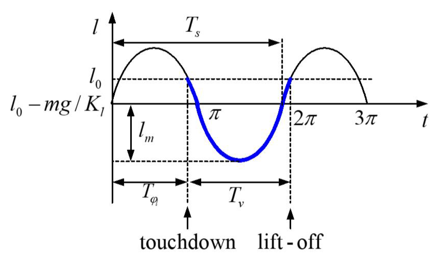
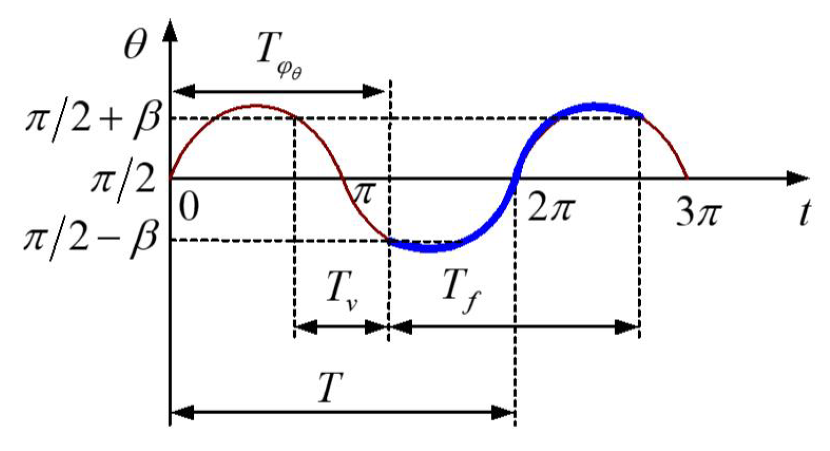
We consider the trajectory tracking problems for the hybrid system (21), (22), (23) or (24). Suppose ${\mathbf{x}}^d\left(t\right)=\mathrm{col}({\mathbf{q}}_x^d,{\mathbf{q}}_s^d)$ is a given target trajectory of the hybrid system (21), (22), (23) or (24) on $t\in \left[0,a\right]$, where $a>0$ is a constant and $\mathrm{col}(,)$ represents a column vector. Define a set $S=\left\{1,2,\dots ,N_{\sigma }\right\}$, where $N_{\sigma }$ denotes the number of the discrete jumps of systems (21), (22), (23) or (24) along the trajectory ${\mathbf{x}}^d\left(t\right)$, and define $t_i=t_i^{+}=t_i^{-}$ ($i\in S$) to be the instant of the state jumps, and $\mathsf{\Delta }{t}_{vc}=t_i^{+}-t_i^{-}=0$ due to the assumption (A3). Let $\mathsf{\Delta }{t}_i=\left[\begin{array}{cc}{t}_{i-1}^{+}& t_i^{-}\end{array}\right]$ with all $\mathsf{\Delta }{t}_i>{\tau }^{*}>0$, where ${\tau }^{*}$ is a constant, and $a={\displaystyle \sum _{i=1}^{N_{\sigma }}}\mathsf{\Delta }{t}_i$; then, based on the basic assumptions, a switching controller for the hybrid systems (21), (22), (23) or (24) can be presented as follows.

Theorem 3.

If the hybrid systems (21), (22), (23) or (24) satisfy the basic assumptions, and, for a given state trajectory ${\mathbf{x}}^d\left(t\right)=\mathrm{col}({\mathbf{x}}_x^d,{\mathbf{x}}_s^d)=\mathrm{col}({\mathbf{q}}_x^d,{\mathbf{q}}_s^d)$ on $t\in \left[0,a\right]$, there exists a set of piecewise controllers ${\mathbf{v}}_{\sigma \left(\mathsf{\Delta }{t}_i\right)}\left(t\right)$, $\sigma \left(\mathsf{\Delta }{t}_{i\in S}\right)\in H$ so that

(A4) 

on the time intervals $t\in \mathsf{\Delta }{t}_{i\in \mathsf{\Omega }\subset S}$ and $\mathsf{\Omega }\ne ⌀$, the errors of the closed-loop subsystem ${\mathbf{e}}_s={\mathbf{x}}_s\left(t\right)-{\mathbf{x}}_s^d\left(t\right)$ controlled by the inputs ${\mathbf{v}}_{\sigma \left(\mathsf{\Delta }{t}_i\right)}\left(t\right)$, $t\in \mathsf{\Delta }{t}_{i\in \mathsf{\Omega }\subset S}$ are globally exponentially stable and meanwhile the errors of the open-loop subsystem ${\mathbf{e}}_x={\mathbf{x}}_x\left(t\right)-{\mathbf{x}}_x^d\left(t\right)$ do not increase, and

(A5) 

on the intervals $t\in \mathsf{\Delta }{t}_{i\in S-\mathsf{\Omega }}$ and $S-\mathsf{\Omega }\ne ⌀$, the errors of the closed-loop subsystem ${\mathbf{e}}_x={\mathbf{x}}_x\left(t\right)-{\mathbf{x}}_x^d\left(t\right)$ controlled by the inputs ${\mathbf{v}}_{\sigma \left(\mathsf{\Delta }{t}_i\right)}\left(t\right)$, $t\in \mathsf{\Delta }{t}_{i\in S-\mathsf{\Omega }}$ are globally exponentially stable and meanwhile the errors of the open-loop subsystem ${\mathbf{e}}_s={\mathbf{x}}_s\left(t\right)-{\mathbf{x}}_s^d\left(t\right)$ do not increase. In addition,

(A6) 

if the hybrid systems (21), (22), (23) or (24) are slow switching systems, that is, the constant ${\tau }^{*}$ is sufficiently large.

Then, systems (21), (22), (23) or (24) can be globally exponentially stabilized to ${\mathbf{x}}^d\left(t\right)$ by the switched controllers ${\mathbf{v}}_{\sigma \left(\mathsf{\Delta }{t}_i\right)}\left(t\right)$ according to the switching sequence $\left(\sigma \left(\mathsf{\Delta }{t}_1\right),\sigma \left(\mathsf{\Delta }{t}_2\right),\dots ,\sigma \left(\mathsf{\Delta }{t}_{N_{\sigma }}\right)\right)$.

Proof. 

For the linear systems (30), the corresponding error systems can be rewritten as

$$\begin{array}{c}\hfill {\dot{\mathbf{e}}}_{\sigma }={\mathbf{A}}_{\sigma }{\mathbf{e}}_{\sigma }+{\tilde{\mathbf{v}}}_{\sigma },\end{array}$$

(31)

where ${\mathbf{e}}_{\sigma }={\mathbf{x}}_{\sigma }\left(t\right)-{\mathbf{x}}_{\sigma }^d\left(t\right)$ and ${\tilde{\mathbf{v}}}_{\sigma }={\mathbf{A}}_{\sigma }{\mathbf{x}}_{\sigma }^d-{\dot{\mathbf{x}}}_{\sigma }^d+{\mathbf{B}}_{\sigma }{\mathbf{v}}_{\sigma }$. Then, by the feedback ${\tilde{\mathbf{v}}}_{\sigma }=-{\mathbf{K}}_{\sigma }{\mathbf{e}}_{\sigma }$, the error systems (31) can be written as

$$\begin{array}{c}\hfill {\dot{\mathbf{e}}}_{\sigma }={\overline{\mathbf{A}}}_{\sigma }{\mathbf{e}}_{\sigma },\end{array}$$

(32)

where the matrices ${\overline{\mathbf{A}}}_{\sigma }={\mathbf{A}}_{\sigma }-{\mathbf{K}}_{\sigma }$ are Hurwitz matrices. Thus, for all $t\in \mathsf{\Delta }{t}_{i\in S}$, the error systems of the closed-loop subsystems satisfy

$$\begin{array}{c}\hfill {∥{\mathbf{e}}_{\sigma }\left(t\right)∥}_{t\in \mathsf{\Delta }{t}_{i\in S}}\le e^{-{\rho }_{i}t}∥{\mathbf{e}}_{\sigma }\left(t_{i-1}\right)∥,\end{array}$$

(33)

where ${\rho }_i>0$ are positive constants that are determined by the characteristic values of the matrices ${\overline{\mathbf{A}}}_{\sigma }$; meanwhile, according to (A4) and (A5), the errors of the open loop subsystems satisfy

$$\begin{array}{c}\hfill {∥{\mathbf{e}}_{\sigma }\left(t\right)∥}_{t\in \mathsf{\Delta }{t}_{i\in S}}\le ∥{\mathbf{e}}_{\sigma }\left(t_{i-1}\right)∥+{\delta }_i,\end{array}$$

(34)

where ${\delta }_i>0$ are constants that are caused by the state jumps of the hybrid systems (21), (22), (23) or (24), and the constants ${\delta }_i$ are finite since the matrix ${\mathbf{M}}_{\mathrm{diag}}\left({\mathbf{q}}_s\right)$ is always positive definite and the norm $∥\mathbf{W}\left(\mathbf{q}\right)∥$ has an upper bound for all smooth constraints Equation (2).

On the other hand, due to $\mathsf{\Omega }\ne ⌀$ and $S-\mathsf{\Omega }\ne ⌀$, on a subsequent interval $\mathsf{\Delta }{t}_{j\in S,j\ne i}$, the state errors ${\delta }_i$ caused by the i-th state jump can be eliminated because of the assumption (A6), which supposes that ${\tau }^{*}$ is sufficiently large. Then, for the given target trajectory ${\mathbf{x}}^d\left(t\right)$ on $t\in \left[0,a\right]$, we can conclude that there exist constants $0<{\overline{\rho }}_i<{\rho }_i$, $i\in S$ so that

$$\begin{array}{c}\hfill \begin{array}{c}{∥\mathbf{e}\left(t_i\right)∥}_{i=N_{\sigma }}\le {∥{\mathbf{e}}_x\left(t_i\right)∥}_{i=N_{\sigma }}+{∥{\mathbf{e}}_s\left(t_i\right)∥}_{i=N_{\sigma }}\hfill \\ \begin{array}{ccc}& & \end{array}\le e^{-{\overline{\rho }}_{N_{\sigma }}{\tau }^{*}}\left({∥{\mathbf{e}}_x\left(t\right)∥}_{i=N_{\sigma }-1}+{∥{\mathbf{e}}_s\left(t\right)∥}_{i=N_{\sigma }-1}\right)\hfill \\ \begin{array}{ccc}& & \end{array}\dots \hfill \\ \begin{array}{ccc}& & \end{array}\le e^{-\left({\displaystyle \sum _{i=1}^{N_{\sigma }}}{\overline{\rho }}_i\right){\tau }^{*}}\left({∥{\mathbf{e}}_x\left(t\right)∥}_{i=1}+{∥{\mathbf{e}}_s\left(t\right)∥}_{i=1}\right)\hfill \\ \begin{array}{ccc}& & \end{array}\le e^{-{\overline{\rho }}_0{\tau }^{*}}\left(∥{\mathbf{e}}_x\left(0\right)∥+∥{\mathbf{e}}_s\left(0\right)∥\right).\hfill \end{array}\end{array}$$

(35)

This completes the proof. □

Remark 4.

Theorem 3 reveals that a class of the underactuated systems with variant constraints can track certain time varying trajectory by switched linear controllers with only partial state feedback in a time-sharing manner, even though the underactuated systems under consideration are generally nonholonomic systems that are possibly caused by either external non-integrable differential constraints or internal dynamics of the passive subsystems (28) and (29). Thus, the presented switched linear controllers are essentially a class of discontinuous nonlinear feedback controllers [27]. It is interesting that the HDS (21), (22), (23) or (24) could be stabilized to a time-varying trajectory by the presented switched linear controller, but the presented controllers could not stabilize the systems (21), (22), (23) or (24) to time invariant equilibrium points since the full state variables should be stabilized simultaneously.

For many applications in practice, energy-efficiency is an important index. On the other hand, from a viewpoint of the closed loop systems, the larger energy consumption in steady motions of a controlled system often means the less of stability margin of the system. Thus, it is useful to search for an energy efficient trajectory of the hybrid systems (21), (22), (23) or (24) so that the stabilizing conditions of the switched linear controllers presented in Theorem 3 could be further relaxed. To this end, we present the following statement.

Theorem 4.

If the hybrid systems (21), (22), (23) or (24) satisfy the basic assumptions, and, for a given state trajectory ${\mathbf{x}}^d\left(t\right)=\mathrm{col}({\mathbf{x}}_x^d,{\mathbf{x}}_s^d)$ on $t\in \left[0,a\right]$, there exists a set of piecewise controllers ${\mathbf{v}}_{\sigma \left(\mathsf{\Delta }{t}_i\right)}\left(t\right)$, $\sigma \left(\mathsf{\Delta }{t}_{i\in S}\right)\in H$ so that

(B1) 

at the instants $t_{i\in S}$, the impulses due to state jumps satisfy $\tilde{\lambda }\left(t_{i\in S}\right)=0$, and

(B2) 

on the time intervals $\mathsf{\Delta }{t}_{i\in \mathsf{\Omega }\subset S},\mathsf{\Omega }\ne ⌀$ and $\mathsf{\Omega }\ne S$, the error convergence rates of the subsystem ${\mathbf{e}}_{\sigma \left(\mathsf{\Delta }{t}_i\right)}$ controlled by the inputs ${\mathbf{v}}_{\sigma \left(\mathsf{\Delta }{t}_i\right)}\left(t\right)$ in closed-loop mode are larger than the error divergence rates of it on the time intervals $\mathsf{\Delta }{t}_{i\in S-\mathsf{\Omega }}$ in open loop mode, and for all state variables, the total time in closed-loop mode equals to that in open loop mode, that is, ${\displaystyle {\displaystyle \sum _{i\in \mathsf{\Omega }}}}\mathsf{\Delta }{t}_i={\displaystyle \sum _{i\in S-\mathsf{\Omega }}}\mathsf{\Delta }{t}_i$. In addition,

(B3) 

if the hybrid systems (21), (22), (23) or (24) are slow switching systems, that is, the constant ${\tau }^{*}$ is sufficiently large.

Then, systems (21), (22), (23) or (24) can be globally exponentially stabilized to ${\mathbf{x}}^d\left(t\right)$ by the switched controllers ${\mathbf{v}}_{\sigma \left(\mathsf{\Delta }{t}_i\right)}\left(t\right)$ according to the switching sequence $\left(\sigma \left(\mathsf{\Delta }{t}_1\right),\sigma \left(\mathsf{\Delta }{t}_2\right),\dots ,\sigma \left(\mathsf{\Delta }{t}_{N_{\sigma }}\right)\right)$.

Proof. 

Referring to systems (23) and (24) and considering the condition (B1), we can see that the state jumps are zero. This is possible since the solutions $\left(\mathbf{q},\dot{\mathbf{q}}\right)$ of the following equations

$$\begin{array}{c}\hfill {\left({\mathbf{W}}^{\mathrm{T}}\left(\mathbf{q}\right){\mathbf{M}}_{}^{-1}\left({\mathbf{q}}_s\right)\mathbf{W}\left(\mathbf{q}\right)\right)}^{-1}{\mathbf{W}}^{\mathrm{T}}\left(\mathbf{q}\right)\dot{\mathbf{q}}\left(t_{vc}^{-}\right)=0\end{array}$$

(36)

and

$$\begin{array}{c}\hfill {\left({\mathbf{W}}^{\mathrm{T}}\left(\mathbf{q}\right){\mathbf{M}}_{}^{-1}\left({\mathbf{q}}_s\right)\mathbf{W}\left(\mathbf{q}\right)\right)}^{-1}{\mathbf{W}}^{\mathrm{T}}\left(\mathbf{q}\right)\dot{\mathbf{q}}\left(t_{vc}^{+}\right)=0\end{array}$$

(37)

generally exist and not unique. Without loss of generality, suppose the closed-loop systems on the intervals $\mathsf{\Delta }{t}_{i\in \mathsf{\Omega }\subset S}$ happen to be the passive subsystems. According to the condition (B2), and referring to Equation (33), the errors of the closed-loop subsystems satisfy

$$\begin{array}{c}\hfill {∥{\mathbf{e}}_x\left(t\right)∥}_{t\in \mathsf{\Delta }{t}_i}\le e^{-{\rho }_{i}t}∥{\mathbf{e}}_x\left(t_{i-1}\right)∥,\end{array}$$

(38)

where ${\rho }_i>0$ are positive constants that can be determined by the characteristic values of the matrices ${\overline{\mathbf{A}}}_{\sigma }$; meanwhile, the errors of the open loop subsystems have relationships

$$\begin{array}{c}\hfill {∥{\mathbf{e}}_s\left(t\right)∥}_{t\in \mathsf{\Delta }{t}_i}\ge e^{{\gamma }_{i}t}∥{\mathbf{e}}_s\left(t_{i-1}\right)∥,\end{array}$$

(39)

where ${\gamma }_i>0$ are also positive constants. On the other intervals, $\mathsf{\Delta }{t}_{i\in S-\mathsf{\Omega }}$, the closed-loop subsystems should be the actuated subsystems, and the errors of the closed-loop subsystems satisfy

$$\begin{array}{c}\hfill {∥{\mathbf{e}}_s\left(t\right)∥}_{t\in \mathsf{\Delta }{t}_i}\le e^{-{\alpha }_{i}t}∥{\mathbf{e}}_s\left(t_{i-1}\right)∥,\end{array}$$

(40)

where ${\alpha }_i>0$ are constants; meanwhile, the errors of the open loop subsystems have relationships

$$\begin{array}{c}\hfill {∥{\mathbf{e}}_x\left(t\right)∥}_{t\in \mathsf{\Delta }{t}_i}\ge e^{{\beta }_{i}t}∥{\mathbf{e}}_x\left(t_{i-1}\right)∥,\end{array}$$

(41)

where ${\beta }_i>0$ are also constants. Note that the four groups’ constants ${\rho }_i$, ${\gamma }_i$, ${\alpha }_i$ and ${\beta }_i$ satisfy the following relationships because of the given condition ${\displaystyle \sum _{i\in \mathsf{\Omega }}}\mathsf{\Delta }{t}_i={\displaystyle \sum _{i\in S-\mathsf{\Omega }}}\mathsf{\Delta }{t}_i$ of (B2),

$$\begin{array}{c}\hfill {\displaystyle \sum _{i\in \mathsf{\Omega }}}\left({\rho }_i\mathsf{\Delta }{t}_i\right)>{\displaystyle \sum _{i\in S-\mathsf{\Omega }}}\left({\beta }_i\mathsf{\Delta }{t}_i\right)\end{array}$$

(42)

and

$$\begin{array}{c}\hfill {\displaystyle \sum _{i\in S-\mathsf{\Omega }}}\left({\alpha }_i\mathsf{\Delta }{t}_i\right)>{\displaystyle \sum _{i\in \mathsf{\Omega }}}\left({\gamma }_i\mathsf{\Delta }{t}_i\right).\end{array}$$

(43)

Therefore, on the interval $\left[0,a\right]$, the errors of systems (21), (22), (23) or (24) can be estimated by

$$\begin{array}{c}\hfill \begin{array}{c}{∥\mathbf{e}\left(t_i\right)∥}_{i=N_{\sigma }}\le {∥{\mathbf{e}}_x\left(t_i\right)∥}_{i=N_{\sigma }}+{∥{\mathbf{e}}_s\left(t_i\right)∥}_{i=N_{\sigma }}\hfill \\ \begin{array}{ccc}& & \end{array}\le e^{\left(-{\displaystyle \sum _{i\in \mathsf{\Omega }}}\left({\rho }_i\mathsf{\Delta }{t}_i\right)+{\displaystyle \sum _{i\in S-\mathsf{\Omega }}}\left({\beta }_i\mathsf{\Delta }{t}_i\right)\right)}∥{\mathbf{e}}_x\left(0\right)∥\hfill \\ \begin{array}{cccc}& & & \end{array}+e^{\left({\displaystyle \sum _{i\in \mathsf{\Omega }}}\left({\gamma }_i\mathsf{\Delta }{t}_i\right)-{\displaystyle \sum _{i\in S-\mathsf{\Omega }}}\left({\alpha }_i\mathsf{\Delta }{t}_i\right)\right)}∥{\mathbf{e}}_s\left(0\right)∥\hfill \\ \begin{array}{ccc}& & \end{array}=e^{{\rho }_0}∥{\mathbf{e}}_x\left(0\right)∥+e^{{\gamma }_0}∥{\mathbf{e}}_s\left(0\right)∥,\hfill \end{array}\end{array}$$

(44)

where

$$\begin{array}{c}\hfill {\rho }_0=-{\displaystyle \sum _{i\in \mathsf{\Omega }}}\left({\rho }_i\mathsf{\Delta }{t}_i\right)+{\displaystyle \sum _{i\in S-\mathsf{\Omega }}}\left({\beta }_i\mathsf{\Delta }{t}_i\right)\end{array}$$

(45)

and

$$\begin{array}{c}\hfill {\gamma }_0={\displaystyle \sum _{i\in \mathsf{\Omega }}}\left({\gamma }_i\mathsf{\Delta }{t}_i\right)-{\displaystyle \sum _{i\in S-\mathsf{\Omega }}}\left({\alpha }_i\mathsf{\Delta }{t}_i\right).\end{array}$$

(46)

From Equation (43), it is directly shown that ${\rho }_0<0$, and ${\gamma }_0<0$. This completes the proof. □

Remark 5.

Theorem 4 shows that the stabilizing conditions presented in Theorem 3 can be relaxed if the motions of the controlled system satisfy the zero impulse condition Equation (27) [28]. In Theorem 4, the open loop subsystems are permitted to be unstable while they satisfy certain conditions. More importantly, by combining Theorems 2 and 4, it is not difficult to find that the hybrid dynamical system (21), (22), (23) or (24) could be stabilized to a smooth periodic orbit that is governed by the nature dynamics of the system while the periodic orbit also satisfies the zero impulse condition Equation (27).

4. Dynamics and Control of Planar One-Legged Hopping Robots

4.1. The Hybrid Dynamics of a Planar One-Legged Hopping Robot

In order to demonstrate the applications of the main results presented in the preceding sections, a planar hopping robot system [4], as shown in Figure 1, is employed to achieve this goal. The hopping robot has a single actuated linear spring leg and a rotational actuated body, and a torsion spring is installed in the hip joint. Suppose the mass of the leg and the body are $m_l$ and $m_b$, respectively, while the foot is massless. The moment of inertia of the leg and the body are $J_l$ and $J_b$, respectively. The length of the leg is l, and its nature length is $l_0$. The spring stiffness of the leg is $k_l$ and the stiffness of the hip spring is $k_h$. For the purpose of simplicity, the center of mass (CM) of the body and the leg are designed just on the hip joint, and the mass of the springs is supposed to be negligible. The generalized coordinates of the hopping system are defined to be $(x,z,\theta ,\phi ,l)$, where $(x,z)$ denotes the position of the foot tip, $\theta$ represents the angle between the leg and the horizontal plane, $\phi$ represents the angle between the body and the leg, and the positive direction of all angular variable is defined to be counter clockwise.

The dynamics of the hopping robot in flight phase can be expressed as

$$\begin{array}{c}\hfill \begin{array}{c}m{\ddot{x}}_{cm}=0,\hfill \\ m{\ddot{z}}_{cm}=-mg,\hfill \\ \left(J_l+J_b\right)\ddot{\theta }+J_b\ddot{\phi }=0,\hfill \\ J_b\ddot{\theta }+J_b\ddot{\phi }+k_h(\phi -{\phi }_0)={\tau }_f,\hfill \end{array}\end{array}$$

(47)

where ${\tau }_f$ is the input torque of the hip joint, and the position of the CM of the robot is given as

$$\begin{array}{c}\hfill \left\{\begin{array}{c}{x}_{cm}=x+lcos\left(\theta \right),\hfill \\ z_{xm}=z+lsin\left(\theta \right).\hfill \end{array}\right.\end{array}$$

(48)

Note that, in flight phase, the length of the leg is $l=l_0$ since the leg can not be controlled in flight phase. Nevertheless, in stance phase, Equations (48) are the holonomic constraints of the hopping robot. Thus, the Jacobian matrix $\mathbf{W}\left(\mathbf{q}\right)$ of Equation (2) can be written as follows by Equation (3):

$$\begin{array}{c}\hfill W\left(q\right)=\left[\begin{array}{cccc}1& 0& lsin\left(\theta \right)& \begin{array}{cc}0& -cos\left(\theta \right)\end{array}\\ 0& 1& -lcos\left(\theta \right)& \begin{array}{cc}0& -sin\left(\theta \right)\end{array}\end{array}\right]\end{array}$$

(49)

and the constraint forces are

$$\begin{array}{c}\hfill \mathit{\lambda }=\mathrm{col}\left({\lambda }_x,{\lambda }_z\right).\end{array}$$

(50)

Thus, the dynamics of the hopping robot in stance phase can be written as

$$\begin{array}{c}\hfill \left\{\begin{array}{c}m{\ddot{x}}_{cm}={\lambda }_x,\hfill \\ m{\ddot{z}}_{cm}=-mg+{\lambda }_z,\hfill \\ \left(J_l+J_b\right)\ddot{\theta }+J_b\ddot{\phi }={\lambda }_{x}lsin\left(\theta \right)-{\lambda }_{z}lcos\left(\theta \right),\hfill \\ J_b\ddot{\theta }+J_b\ddot{\phi }+k_h(\phi -{\phi }_0)={\tau }_s,\hfill \\ {\lambda }_{x}cos\left(\theta \right)+{\lambda }_{z}sin\left(\theta \right)=0.\hfill \end{array}\right.\end{array}$$

(51)

By the constraint Equation (48) and the first two equations of Equation (51), the constraint forces $\left({\lambda }_x,{\lambda }_z\right)$ can be resolved, and then the dynamics Equation (51) can be simplified to

$$\begin{array}{c}\hfill \left\{\begin{array}{c}\left(J_l+J_b+m{l}^2\right)\ddot{\theta }+J_b\ddot{\phi }+2ml\dot{l}\dot{\theta }+mglcos\left(\theta \right)=0,\hfill \\ J_b\ddot{\theta }+J_b\ddot{\phi }+k_h(\phi -{\phi }_0)={\tau }_s,\hfill \\ m\left(\ddot{l}-l{\dot{\theta }}^2\right)+mgsin\left(\theta \right)+k_l(l-l_0)=F.\hfill \end{array}\right.\end{array}$$

(52)

We can verify that the dynamics Equation (52) are the same as that derived directly from the Euler–Lagrange equations. In order to get the equations of the state jumps for the hopping robot, from Equation (11), we have

$$\begin{array}{c}\hfill \left\{\begin{array}{c}m\mathsf{\Delta }{\dot{x}}_{cm}={\tilde{\lambda }}_x,\hfill \\ m\mathsf{\Delta }{\dot{z}}_{cm}={\tilde{\lambda }}_z,\hfill \\ \left(J_l+J_b\right)\mathsf{\Delta }\dot{\theta }={\tilde{\lambda }}_{x}lsin\theta -{\tilde{\lambda }}_{z}lcos\left(\theta \right),\hfill \\ J_b\mathsf{\Delta }\dot{\phi }=0,\hfill \end{array}\right.\end{array}$$

(53)

where

$$\begin{array}{c}\hfill \left\{\begin{array}{c}{\tilde{\lambda }}_x=-psin\left(\theta \right),\hfill \\ {\tilde{\lambda }}_z=pcos\left(\theta \right),\hfill \end{array}\right.\end{array}$$

(54)

since the impulse p is perpendicular to the longitudinal axis of the leg, while, along the axis of the leg, the impulse can be absorbed by the springs of the robot. Substituting Equation (54) into Equation (53), it follows that

$$\begin{array}{c}\hfill \left\{\begin{array}{c}m\mathsf{\Delta }{\dot{x}}_{cm}=-psin\left(\theta \right),\hfill \\ m\mathsf{\Delta }{\dot{z}}_{cm}=pcos\left(\theta \right),\hfill \\ \left(J_l+J_b\right)\mathsf{\Delta }\dot{\theta }=-p{l}_0,\hfill \\ J_b\mathsf{\Delta }\dot{\phi }=0.\hfill \end{array}\right.\end{array}$$

(55)

Then, during the constraint variation interval $\mathsf{\Delta }{t}_{vc}=t_{vc}^{+}-t_{vc}^{-}$, the changes of the speed of the generalized coordinates can be written from Equation (55) as

$$\begin{array}{c}\hfill \left\{\begin{array}{c}{\dot{x}}_{cm}\left(t_{vc}^{+}\right)={\dot{x}}_{cm}\left(t_{vc}^{-}\right)-\frac{sin\left[\theta \left(t_{vc}^{\pm }\right)\right]}{m}p,\hfill \\ {\dot{z}}_{cm}\left(t_{vc}^{+}\right)={\dot{z}}_{cm}\left(t_{vc}^{-}\right)+\frac{cos\left[\theta \left(t_{vc}^{\pm }\right)\right]}{m}p,\hfill \\ \dot{\theta }\left(t_{vc}^{+}\right)=\dot{\theta }\left(t_{vc}^{-}\right)-\frac{l_0}{J_l+J_b}p,\hfill \\ \dot{\phi }\left(t_{vc}^{+}\right)=\dot{\phi }\left(t_{vc}^{-}\right),\hfill \end{array}\right.\end{array}$$

(56)

where $\theta \left(t_{vc}^{\pm }\right)$ denotes $\theta \left(t_{vc}^{+}\right)=\theta \left(t_{vc}^{-}\right)$. On the other hand, from the constraint Equation (48), it is easy to show

$$\begin{array}{c}\hfill \left\{\begin{array}{c}{\dot{x}}_{cm}\left(t_{vc}^{+}\right)-\dot{l}\left(t_{vc}^{+}\right)cos\left[\theta \left(t_{vc}^{\pm }\right)\right]+l_0\dot{\theta }\left(t_{vc}^{+}\right)sin\left[\theta \left(t_{vc}^{\pm }\right)\right]=0,\hfill \\ {\dot{z}}_{cm}\left(t_{vc}^{+}\right)-\dot{l}\left(t_{vc}^{+}\right)sin\left[\theta \left(t_{vc}^{\pm }\right)\right]-l_0\dot{\theta }\left(t_{vc}^{+}\right)cos\left[\theta \left(t_{vc}^{\pm }\right)\right]=0.\hfill \end{array}\right.\end{array}$$

(57)

From Equation (57), it can be deduced that

$$\begin{array}{c}\hfill {\dot{x}}_{cm}\left(t_{vc}^{+}\right)sin\left[\theta \left(t_{vc}^{\pm }\right)\right]-{\dot{z}}_{cm}\left(t_{vc}^{+}\right)cos{\left[\theta \left(t_{vc}^{\pm }\right)\right]}^{}+l_0\dot{\theta }\left(t_{vc}^{+}\right)=0.\end{array}$$

(58)

Substituting Equation (56) into Equation (58) and doing some simple calculations, the impulse can be calculated as

$$\begin{array}{c}\hfill p=\frac{m\left(J_l+J_b\right)}{\left(J_l+J_b\right)+m{l}_0^2}\chi \left(t_{vc}^{-}\right),\end{array}$$

(59)

where

$$\begin{array}{c}\hfill \begin{array}{c}\chi \left(t_{vc}^{-}\right):={\dot{x}}_{cm}\left(t_{vc}^{-}\right)sin\left[\theta \left(t_{vc}^{\pm }\right)\right]-{\dot{z}}_{cm}\left(t_{vc}^{-}\right)cos\left[\theta \left(t_{vc}^{\pm }\right)\right]+l_0\dot{\theta }\left(t_{vc}^{-}\right).\hfill \end{array}\end{array}$$

(60)

Then, substituting Equation (59) into Equation (56), the equations of state jumps caused by the constraint variations can be given as

$$\begin{array}{c}\hfill \left\{\begin{array}{c}{\dot{x}}_{cm}\left(t_{vc}^{+}\right)={\dot{x}}_{cm}\left(t_{vc}^{-}\right)-\frac{\left(J_l+J_b\right)sin\left[\theta \left(t_{vc}^{\pm }\right)\right]}{\left(J_l+J_b\right)+m{l}_0^2}\chi \left(t_{vc}^{-}\right),\hfill \\ {\dot{z}}_{cm}\left(t_{vc}^{+}\right)={\dot{z}}_{cm}\left(t_{vc}^{-}\right)+\frac{\left(J_l+J_b\right)cos\left[\theta \left(t_{vc}^{\pm }\right)\right]}{\left(J_l+J_b\right)+m{l}_0^2}\chi \left(t_{vc}^{-}\right),\hfill \\ \dot{\theta }\left(t_{vc}^{+}\right)=\dot{\theta }\left(t_{vc}^{-}\right)-\frac{m{l}_0}{\left(J_l+J_b\right)+m{l}_0^2}\chi \left(t_{vc}^{-}\right),\hfill \\ \dot{\phi }\left(t_{vc}^{+}\right)=\dot{\phi }\left(t_{vc}^{-}\right),\hfill \end{array}\right.\end{array}$$

(61)

and $\dot{l}\left(t_{vc}^{+}\right)={\dot{x}}_{cm}\left(t_{vc}^{+}\right)cos\theta \left(t_{vc}^{\pm }\right)+{\dot{z}}_{cm}\left(t_{vc}^{+}\right)sin\theta \left(t_{vc}^{\pm }\right)$ for adding constraints due to Equation (57), and $\dot{l}\left(t_{vc}^{+}\right)=0$ for reducing constraints. Thus, the hybrid dynamics of the hopping robot are composed of Equations (47), (52) and (61).

4.2. Motion Planning for the One-Legged Hopping Robots in Steady Locomotion

By introducing springs into the hopping robots, as shown in [29], it is possible for the robots to realize steady hop motions without using large control inputs, while the steady motions are primarily governed by the nature dynamics of the dynamical systems. As seen in the last subsection, the hopping robots are hybrid dynamical systems and the variant constraints of a locomotion system generally result in large state jumps that can easily destroy the stability of the controlled system. In order to realize energy efficient locomotion so that the control inputs can be reduced to a reasonable level and the stability of motions could be improved effectively, it is necessary to carefully plan the target locomotion trajectory of the hopping robot.

A steady continuous motion process of the hopping robots is commonly a periodic motion, which is roughly composed of two harmonic oscillators with different nature frequency, and every motion cycle is composed of four phases, flight phase, touchdown, stance phase, and lift off. During flight and stance phases, the motions of the hopping systems can be controlled, while, in touchdown and lift off phases, the hopping systems can not be controlled due to the short intervals of constraint changes. During stance phases, the nature frequency of the spring leg is

$$\begin{array}{c}\hfill {\omega }_l=\sqrt{k_l/\phantom{k_{l}m}m},\end{array}$$

(62)

so the resonance time period of the linear spring leg is

$$\begin{array}{c}\hfill T_s=2\pi /\phantom{2\pi {\omega }_l}{\omega }_l=2\pi \sqrt{m/\phantom{m{k}_l}{k}_l}.\end{array}$$

(63)

As illustrated in Figure 2, the thick line segment represents the time-amplitude curve of the linear spring leg in stance phase of a motion cycle. Suppose the length of the leg at the instants of touchdown and lift off is the nature length $l_0$, the duration of stance phase is $T_v$, the initial phase-angle of the harmonic vibration of the leg is ${\varphi }_l$, and the vibration amplitude of the spring leg is $l_m$, then the oscillations of the linear leg in stance phases can be approximately expressed by

$$\begin{array}{c}\hfill l\left(t\right)=\left(l_0-mg/\phantom{mg{k}_l}{k}_l\right)+l_{m}sin({\omega }_{l}t+{\varphi }_l),l\left(0\right)=l_0,\end{array}$$

(64)

and the speed of the linear leg is approximately given by

$$\begin{array}{c}\hfill \dot{l}\left(t\right)=l_m{\omega }_{l}cos({\omega }_{l}t+{\varphi }_l),\dot{l}\left(0\right)=\dot{l}\left(t_{vc}^{+}\right),\end{array}$$

(65)

where $\dot{l}\left(t_{vc}^{+}\right)$ is the compress speed of the linear leg at just after the touchdown. By using the two initial conditions of Equations (64) and (65), the two undetermined parameters $l_m$ and ${\varphi }_l$ can be resolved as

$$\begin{array}{c}\hfill {\varphi }_l=\pi -\mathrm{atan}\left(\left|\frac{mg{\omega }_l}{k_l\dot{l}\left(t_{vc}^{+}\right)}\right|\right),l_m=\frac{mg}{k_{l}sin\left({\varphi }_l\right)}.\end{array}$$

(66)

From Figure 2, the duration of a stance phase can be calculated as

$$\begin{array}{c}\hfill T_v=\frac{1}{2}{T}_s+2t_{{\varphi }_l},\end{array}$$

(67)

where $t_{{\varphi }_l}=\frac{1}{{\omega }_l}\mathrm{asin}\left(\frac{mg}{k_l{l}_m}\right)$.

Both in stance phase and flight phase, the vibrations of the hip joint should follow the same harmonic oscillation, but with different initial phase angles. By the dynamics of the hopping robot in flight phases Equation (47), the nature frequency of the hip joint can be calculated as

$$\begin{array}{c}\hfill {\omega }_h=\sqrt{k_h\left(1/\phantom{1J_b+1/\phantom{1J_l}{J}_l}{J}_b+1/\phantom{1J_l}{J}_l\right)}.\end{array}$$

(68)

However, the duration of a flight phase is determined by the lift off speed of the robot, and is given as

$$\begin{array}{c}\hfill T_f=2{\dot{z}}_{lo}/\phantom{2{\dot{z}}_{lo}g}g.\end{array}$$

(69)

Then, the time period of the hopping motions is

$$\begin{array}{c}\hfill T=T_v+T_f=\frac{2\pi }{{\omega }_h}.\end{array}$$

(70)

Similar to Figure 2, the angular motions of the body and the leg can be analyzed in Figure 3, where the thick line segment denotes the flight phase in a hop cycle. From Figure 3, it is easy to show that the angle trajectory of the leg in the flight phases can be written as

$$\begin{array}{c}\hfill \theta \left(t\right)=\frac{\pi }{2}+Asin({\omega }_{h}t+{\varphi }_{\theta })\end{array}$$

(71)

and satisfy the boundary conditions

$$\begin{array}{c}\hfill \theta \left(0\right)=\frac{\pi }{2}-\beta ,\theta (-T_v)=\frac{\pi }{2}+\beta ,\end{array}$$

(72)

where $\beta$ is the swing amplitude of the leg in the hop cycles and is always given by the control commands.

By using the initial conditions Equation (72), the undetermined parameters A and ${\varphi }_{\theta }$ of Equation (71) can be resolved as

$$\begin{array}{c}\hfill {\varphi }_{\theta }=\pi -\frac{1}{2}{\omega }_h{T}_v,A=\frac{\beta }{sin\left({\varphi }_{\theta }\right)}\end{array}$$

(73)

for the stance phases $t\in \left[\begin{array}{cc}0& T_v\end{array}\right]$, and

$$\begin{array}{c}\hfill {\varphi }_{\theta }=\pi +\frac{1}{2}{\omega }_h{T}_v,A=\frac{\beta }{sin\left({\varphi }_{\theta }\right)}\end{array}$$

(74)

for the flight phases $t\in \left[\begin{array}{cc}0& T_f\end{array}\right]$. Since during the flight phases the angular motions of the hopping robots satisfy the law of angular momentum conservation, from Equation (47), the angular speed of the body is determined by

$$\begin{array}{c}\hfill \dot{\phi }\left(t\right)=-\frac{J_b+J_l}{J_b}\dot{\theta }\left(t\right),\end{array}$$

(75)

where we suppose the initial angular momentum of the robot at lift off is zero. The angular position of the body should be

$$\begin{array}{c}\hfill \phi \left(t\right)=\frac{\pi }{2}-\frac{J_b+J_l}{J_b}Asin({\omega }_{h}t+{\varphi }_{\theta }),\end{array}$$

(76)

and the parameters A and ${\varphi }_{\theta }$ in Equation (76) are given by Equation (73) for the stance phases, and given by Equation (74) for the flight phases. Note that there already exists a phase difference $\pi$ in Equations (71) and (76) since the speed directions of the body and the leg are contrary.

4.3. Hopping Control of the One-Legged Planar Robot

As shown in Section 3, for a hybrid dynamical system, it is possible to control the system to certain time varying trajectories by partial state feedback and time-sharing patterns. For the one-legged hopping robot system considered in this paper, the time of continuous dynamics modes (stance and flight phases) is very limited, which do not exactly satisfy the condition (A6) of Theorem 3 or (B3) of Theorem 4. Thus, the state jumps caused by the constraint variations of the hybrid systems can quickly destroy the stability of the closed-loop hybrid systems. However, for the one-legged hopping robot system such as that illustrated in Figure 1, we can use the following two level control approaches to stabilize the periodic hopping systems.

During the continuous dynamics modes, linear controllers with only partial state feedback are utilized on the basis of the Theorems 3 and 4. That is, in stance phases, the variables $l\left(t\right)$ and $\phi \left(t\right)$ of the robot will be controlled to their target motions, while the rotational motions $\theta \left(t\right)$ of the leg will be open loop. Thus, the controller in stance phases is

$$\begin{array}{c}\hfill \left\{\begin{array}{c}{\tau }_s=J_b\left(1-\frac{1}{J_l+J_b+m{l}^2}\right)\left({\ddot{\phi }}^d\left(t\right)-k_1{e}_{\phi }-k_2{\dot{e}}_{\phi }\right)\hfill \\ \begin{array}{cc}& \end{array}-\frac{J_b\left[2ml\dot{l}\dot{\theta }+mglcos\left(\theta \right)\right]}{J_l+J_b+m{l}^2}+k_h(\phi -{\phi }_0),\hfill \\ F=m\left({\ddot{l}}^d\left(t\right)-k_3{e}_l-k_4{\dot{e}}_l\right)-ml{\dot{\theta }}^2+mgsin\left(\theta \right)\hfill \\ +k_l(l-l_0),\hfill \end{array}\right.\end{array}$$

(77)

where $e_{\phi }=\phi \left(t\right)-{\phi }^d\left(t\right)$, $e_l=l\left(t\right)-l^d\left(t\right)$, $t\in \left[\begin{array}{cc}0& T_v\end{array}\right]$, and $k_i$ $(i=1,\dots ,4)$ are positive constants. In flight phases, the angle of the leg is only controlled to the given trajectory ${\theta }^d\left(t\right)$ in closed loop so that the robot lands in right states, while the body is actuated in open loop by the opposite reaction of the leg. In flight phase, the length of the leg does not change, i.e., $l\left(t\right)=l_0$. Thus, the controller in flight phases is given by

$$\begin{array}{c}\hfill {\tau }_f=-J_l\left({\ddot{\theta }}^d\left(t\right)-k_5{e}_{\theta }-k_6{\dot{e}}_{\theta }\right)+k_h(\phi -{\phi }_0),\end{array}$$

(78)

where $e_{\theta }=\theta \left(t\right)-{\theta }^d\left(t\right)$, $t\in \left[\begin{array}{cc}0& T_f\end{array}\right]$; $k_5$ and $k_6$ are also two positive constants. Note that the feedback gains $k_i$$(i=1,\dots ,6)$ can easily be obtained by the approaches of linear quadratic optimal regulators (LQR). In order to stabilize the one-legged robots to a desired periodic orbit trajectory, an adaptive controller with discrete time feedback is applied to stabilize the leg’s attitude in stance phases

$$\begin{array}{c}\hfill \begin{array}{c}{\theta }_{\mathrm{th}}\left(k\right)={\theta }_0+r_2\left(k\right)E_{{\theta }_{lo}}\left(k\right)+r_{3}D{E}_{{\theta }_{lo}}\left(k\right),\hfill \\ r_2\left(k\right)=r_0+r_1\chi \left(k\right),\hfill \end{array}\end{array}$$

(79)

where k is the current times of touchdown, ${\theta }_{\mathrm{th}}\left(k\right)$ is the desired angle of the leg at the instant of touchdown, $E_{{\theta }_{lo}}\left(k\right)={\theta }_{lo}\left(k\right)-{\theta }_{lo}(k-1)$ is the change of the leg angle at the instant of lift off, and $D{E}_{{\theta }_{lo}}\left(k\right)$ is defined to be $D{E}_{{\theta }_{lo}}\left(k\right)=E_{{\theta }_{lo}}\left(k\right)-E_{{\theta }_{lo}}(k-1)$, $r_0$, $r_1$ and $r_3$ are adjustable positive constants, and ${\theta }_0$ is determined by the desired locomotion speed of the robot and is approximately given by ${\theta }_0=\frac{\pi }{2}+\mathrm{atan}\left(\frac{{\dot{x}}_{cm}{T}_v}{2l_0}\right)$.

Suppose the physical parameters of the robot model as that given in

Table 1. The model parameters of the hopping robot.

Name	Symbol	Value	Unit
Mass	m	12.0	kg
Gravity acceleration	g	9.8	m/s${}^2$
Nature length of leg	$l_0$	0.531	m
Inertia of body	$J_b$	0.8	kgm${}^2$
Inertia of leg	$J_l$	0.15	kgm${}^2$
Stiffness of leg spring	$K_l$	3000	N/m
Stiffness of hip spring	$K_h$	10	Nm/rad

, and the initial states of the robot are given by

$$\begin{array}{c}\hfill \begin{array}{c}{\left(x_{cm},z_{cm},\theta ,\phi ,l,{\dot{x}}_{cm},{\dot{z}}_{cm},\dot{\theta },\dot{\phi },\dot{l}\right)}_{t=0}=\hfill \\ \left(0,1.0,\frac{\pi }{2}-\frac{10\pi }{180},\frac{\pi }{2}+\frac{10\pi }{180},0.531,1.7,0,0,0,0\right),\hfill \end{array}\end{array}$$

(80)

where ${\left(x_{cm},z_{cm}\right)}_{t=0}=\left(0,1.0\right)$ is the initial position of the CM of the robot, ${\left(\theta ,\phi ,l\right)}_{t=0}=\left(\frac{\pi }{2}-\frac{10\pi }{180},\frac{\pi }{2}+\frac{10\pi }{180},0.531\right)$ is a given initial configuration of the robot, ${\left({\dot{x}}_{cm},{\dot{z}}_{cm},\dot{\theta },\dot{\phi },\dot{l}\right)}_{t=0}=\left(1.7,0,0,0,0\right)$ is the initial speed of the robot. Then, by applying the linear controllers (77), (78) and (79), some numerical simulation results of stabilizing the hopping robot to locomotion with moving speed about 2.0 m/s are illustrated in Figure 4, Figure 5, Figure 6, Figure 7, Figure 8 and Figure 9. Differential equations are solved by employing the well-known Runge-Kutta algorithm.

Figure 4 shows the trajectories of the variables $\left(\theta ,\phi ,l\right)$ in the last three cycles of fifty hops in total, Figure 5 illustrates the corresponding control inputs, and Figure 6 plots the animations of the robot in the last three hops. The state jumps measure Equation (60) of the controlled robot system is illustrated in Figure 7, which shows that the state jumps at touchdown phase finally converge to zero. In other words, the hopping robot is stabilized to a periodic orbit with zero impulse at touchdown phases, so that the energy efficiency of the hopping system is improved and the maximum of the inputs is reduced to a reasonable level (referring to Figure 5); otherwise, the maximum of the inputs will be very large under closed-loop mode. However, the nonzero inputs of the robot in stable hops are caused by the approximate target trajectory Equation (64) since the spring leg in stance phase is actually an oscillating system with variant stiffness. Referring to Equation (52), the actual equivalent stiffness of the linear spring leg should be ${\overline{k}}_l=k_l-m\dot{\theta }{\left(t\right)}^2$. In addition, as examples, Figure 8 and Figure 9 also respectively show that the state variables $\left(l\left(t\right),\dot{l}\left(t\right)\right)$ and $\left(\theta \left(t\right),\dot{\theta }\left(t\right)\right)$ are stabilized to a period one orbit.

5. Conclusions

From the viewpoint of Lagrange–d’Alembert equations with additional constraints, this paper investigates the modeling approaches of a class of VCS with instantaneously variant constraints, and the switching control techniques of stabilizing the VCS to given periodic orbits. We show that under certain conditions the VCS are essentially a class of HDS, and there possibly exist periodic orbits with zero impacts, so that the HDS can be stabilized to period-one orbits by linear controllers with partial state feedback, even though the HDS are generally underactuated nonholonomic systems in time continuous modes. These new discoveries point out that:

(a)

in an HDS, there generally exist time-varying trajectories without impacts, and,

(b)

if the zero impact trajectories are physically meaningful, then the controlled HDS can be stabilized to the zero impact trajectories by simple switched linear controllers, and

(c)

the zero impact trajectories provide high energy efficient locomotion modes since the energy loss caused by impacts is avoided.

In addition, by a one-legged planar hopping robot, the main results of modeling and control approaches for the HDS are discussed in detail, and the numerical simulation results are in good agreement with the conclusions of this paper. In order to use the proposed control approach in practice, improving the robust stability of the closed-loop system and applying the pulse control [30] should be further considered.

References

1. Goebel, R.; Sanfelice, R.; Teel, A. Hybrid dynamical systems: Robust stability and control for systems that combine continuoustime and discrete-time dynamics. IEEE Control Syst. Mag. 2009, 29, 28–83. [Google Scholar] [CrossRef]
2. Martinez-Garcia, M.; Zhang, Y.; Gordon, T. Modeling lane keeping by a hybrid open-closed-loop pulse control scheme. IEEE Trans. Ind. Inform. 2016, 12, 2256–2265. [Google Scholar] [CrossRef]
3. Schaft, A.; Schumacher, H. An Introduction to Hybrid Dynamical Systems; Springer: London, UK, 2000. [Google Scholar]
4. Hyon, S.H.; Emura, T. Energy-preserving control of a passive one-legged running robot. Adv. Robot. 2004, 18, 357–381. [Google Scholar] [CrossRef] [Green Version]
5. Sadati, N.; Dumont, G.A.; Hamed, K.A.; Gruver, W.A. Hybrid Control and Motion Planning of Dynamical Legged Locomotion; JohnWiley and Sons: Hoboken, NJ, USA, 2012; Volume 2. [Google Scholar]
6. Hurmuzlu, Y.; Marghitu, D.B. Rigid body collisions of planar kinematic chains with multiple contact points. Int. J. Robot. Res. 1994, 13, 82–92. [Google Scholar] [CrossRef]
7. Hurmuzlu, Y.; GéNot, F.; Brogliato, B. Modeling, stability and control of biped robots: A general framework. Automatica 2004, 40, 1647–1664. [Google Scholar] [CrossRef]
8. Grizzle, J.W.; Abba, G.; Plestan, F. Asymptotically stable walking for biped robots: Analysis via systems with impulse effects. IEEE Trans. Autom. Control 2001, 46, 51–64. [Google Scholar] [CrossRef]
9. Grizzle, J.; Moog, C.H.; Chevallereau, C. Nonlinear control of mechanical systems with an unactuated cyclic variable. IEEE Trans. Autom. Control 2005, 50, 559–576. [Google Scholar] [CrossRef] [Green Version]
10. Liao, H. Nonlinear dynamics of duffing oscillator with time delayed term. CMES Comput. Model. Eng. Sci 2014, 103, 155–187. [Google Scholar]
11. Bloch, A.M. Nonholonomic mechanics. In Nonholonomic Mechanics and Control; Springer: New York, NY, USA, 2003; pp. 207–276. [Google Scholar]
12. Brockett, R.W. Asymptotic stability and feedback stabilization. Differ. Geom. Control Theory 1983, 27, 181–191. [Google Scholar]
13. He, G.; Geng, Z. Dynamics synthesis and control for a hopping robot with articulated leg. Mech. Mach. Theory 2011, 46, 1669–1688. [Google Scholar] [CrossRef]
14. M’ Closkey, R.; Morin, P. Time-varying homogeneous feedback: Design tools for the exponential stabilization of systems with drift. Int. J. Control 1998, 71, 837–869. [Google Scholar] [CrossRef]
15. Reyhanoglu, M. Exponential stabilization of an underactuated autonomous surface vessel. Automatica 1997, 33, 2249–2254. [Google Scholar] [CrossRef] [Green Version]
16. He, G.; Zhang, C.; Sun, W.; Geng, Z. Stabilizing the second-order nonholonomic systems with chained form by finite-time stabilizing controllers. Robotica 2016, 34, 2344–2367. [Google Scholar] [CrossRef]
17. Xu, W.; Ma, B.L. Stabilization of second-order nonholonomic systems in canonical chained form. Robot. Auton. Syst. 2001, 34, 223–233. [Google Scholar] [CrossRef]
18. Tian, Y.P.; Li, S. Exponential stabilization of nonholonomic dynamic systems by smooth time-varying control. Automatica 2002, 38, 1139–1146. [Google Scholar] [CrossRef]
19. Liu, Y.; Zang, X.; Heng, S.; Lin, Z.; Zhao, J. Human-Like Walking with Heel Off and Toe Support for Biped Robot. Appl. Sci. 2017, 7, 499. [Google Scholar] [CrossRef]
20. Jiang, Z.; Yan, P. Asynchronous switching control for continuous-time switched linear systems with output-feedback. Int. J. Control. Autom. Syst. 2018, 16, 2082–2092. [Google Scholar] [CrossRef]
21. Filippov, A.F. Differential Equations with Discontinuous Righthand Sides: Control Systems; Springer: Berlin, Germany, 2013; Volume 18. [Google Scholar]
22. Lin, H.; Antsaklis, P.J. Stability and stabilizability of switched linear systems: A survey of recent results. IEEE Trans. Autom. Control 2009, 54, 308–322. [Google Scholar] [CrossRef]
23. Yang, H.; Jiang, B.; Cocquempot, V. Stabilization of Switched Nonlinear Systems with Unstable Modes; Springer: Heidelberg, Germany, 2014; Volume 9. [Google Scholar]
24. Marsden, J.E.; Ratiu, T.S. Introduction to Mechanics and Symmetry: A Basic Exposition of Classical Mechanical Systems; Springer Science and Business Media: Berlin/Heidelberg, Germany, 2013; Volume 17. [Google Scholar]
25. Olfati-Saber, R. Normal forms for underactuated mechanical systems with symmetry. IEEE Trans. Autom. Control 2002, 47, 305–308. [Google Scholar] [CrossRef]
26. Levine, J. Analysis and Control of Nonlinear Systems: A Flatness-Based Approach; Springer: Berlin/Heidelberg, Germany, 2009. [Google Scholar]
27. Orlov, Y.V. Discontrinuous Systems: Lyaponov Analysis and Robust Synthesis under Uncertainty Conditions; Springer: London, UK, 2009. [Google Scholar]
28. Hereid, A.; Hubicki, C.M.; Cousineau, E.A.; Ames, A.D. Dynamic humanoid locomotion: A scalable formulation for hzd gait optimization. IEEE Trans. Robot. 2018, 34, 370–387. [Google Scholar] [CrossRef]
29. Ahmadi, M.; Buehler, M. Controlled passive dynamic running experiments with the ARL-monopod II. IEEE Trans. Robot. 2006, 22, 974–986. [Google Scholar] [CrossRef]
30. Zhang, Y.; Gordon, T.; Martinez-Garcia, M.; Bingham, C. Steering measurement decomposition for vehicle lane keeping—A study of driver behaviour. Measurement 2018, 121, 26–38. [Google Scholar] [CrossRef]
Figure 1. Model of a planar one-legged hopping robot.
Applsci 09 04235 g001
Figure 2. Diagram of harmonic vibration of the linear spring leg.
Applsci 09 04235 g002
Figure 3. Diagram of the angular motions of the hopping robot.
Applsci 09 04235 g003
Figure 4. Coordinate trajectories of the robot in a stable hopping orbit.
Applsci 09 04235 g004
Figure 5. The inputs of the robot in a stable hopping orbit.
Applsci 09 04235 g005
Figure 6. Animations of the one-legged robots in hooping with locomotion speed about 2 m/s.
Applsci 09 04235 g006
Figure 7. Values of the state jumps measure (60) of the one-legged robots.
Applsci 09 04235 g007
Figure 8. The stable orbit of the variable l ( t ) .
Applsci 09 04235 g008
Figure 9. The stable orbit of the variable θ ( t ) .
Applsci 09 04235 g009