Multi-Switching Combination Synchronization of Three Fractional-Order Delayed Systems


1
School of Computer Science and Engineering, Southeast University, Nanjing 211189, China
2
School of Information Science and Engineering, Yunnan University, Kunming 650091, China
*
Author to whom correspondence should be addressed.
Appl. Sci. 2019, 9(20), 4348; https://0-doi-org.brum.beds.ac.uk/10.3390/app9204348
Submission received: 19 July 2019
/
Revised: 8 August 2019
/
Accepted: 13 August 2019
/
Published: 15 October 2019
(This article belongs to the Special Issue Mathematical Modeling using Differential Equations, and Network Theory)
Abstract
:Multi-switching combination synchronization of three fractional-order delayed systems is investigated. This is a generalization of previous multi-switching combination synchronization of fractional-order systems by introducing time-delays. Based on the stability theory of linear fractional-order systems with multiple time-delays, we propose appropriate controllers to obtain multi-switching combination synchronization of three non-identical fractional-order delayed systems. In addition, the results of our numerical simulations show that they are in accordance with the theoretical analysis.
1. Introduction
Fractional calculus has attracted researchers from various fields due to fractional dimensions widely existing in nature and engineering fields [1,2,3]. Compared to the integer-order dynamical systems, the fractional-order counterparts can exhibit more complex dynamical behaviors. Some of the researches on integer-order dynamical systems can be generalized to fractional-order dynamical systems. Fractional-order dynamical systems have been widely investigated, such as synchronization [4], identification [5], stabilization [6] and approximate entropy analysis [7,8]. Time-delay is a frequently encountered phenomenon in real applications, such as physical, communication, economical, pneumatic and biological systems [9]. Introducing time-delay into a system can enrich its dynamic characteristics and describe a real-life phenomenon more precisely. Thus, the fractional-order delayed differential equation (FDDE) is becoming a hot topic for scientists and engineers, and it has many theoretical and practical applications [10]. Nowadays, the chaotic behavior and synchronization of FDDE attract intensive research interests. In [11], Bhalekar et al. introduced the fractional-order delayed Liu system. The fractional-order delayed financial system was presented in [12], and hybrid projective synchronization between the aforementioned two systems was achieved in [13]. The fractional-order delayed Chen system was proposed in [14], while its adaptive synchronization was investigated in [15]. The fractional-order delayed porous media was proposed in [16]. In [17], a fractional-order delayed Newton–Leipnik system was taken as an example to present intermittent synchronizing delayed fractional nonlinear system.
Due to its wide applications in secure communication, synchronization of fractional-order delayed chaotic systems are extensively investigated [18,19,20,21]. However, all the above-mentioned and other synchronization schemes are in traditional drive–response ways, which only have unique drive and response systems. Recently, Luo et al. [22] extended the traditional drive–response synchronization to combination synchronization, which has two drive systems and one response system. Compared to the drive–response synchronization, combination synchronization has stronger anti-decode and anti-attack abilities in image encryption and secure communication, in which origin messages are split into two parts and each part can be embedded into two separate drive systems. There are many works on combination synchronization [23,24,25,26]. To further strengthen the security in secure communication, Vincent et al. [27] proposed multi-switching combination synchronization scheme, in which the two drive systems are synchronized with the response system in different states. Based on the nonlinear control technique, Zheng [28] studied multi-switching combination synchronization of three non-identical chaotic systems. Khan [29] investigated adaptive multi-switching combination synchronization among three non-identical chaotic systems. In [30], Ahmad et al. proposed globally exponential multi-switching combination synchronization scheme, and applied it to secure communications. Multi-switching combination synchronization was applied in encrypted audio communication in [31]. The previous work on multi-switching combination synchronization schemes are based on integral-order chaotic systems. To improve the security in these synchronization schemes, based on fractional-order chaotic systems, Bhat et al. [32] extended the work in [27] to study multi-switching combination synchronization among three non-identical fractional-order chaotic systems. Khan et al. [33] investigated multi-switching combination-combination synchronization among a class of four non-identical fractional-order chaotic systems. In multi-switching combination-combination synchronization scheme, the state variables of two drive systems synchronize with different state variables of two response systems simultaneously, which makes the security of this scheme higher than that in [32].
Since time-delay is a frequently encountered phenomenon in real applications, and the time-delay can be used as an additional parameter in synchronization to increase security in secure communication, we consider the work in [32] to investigate multi-switching combination synchronization scheme for non-identical fractional-order delayed systems by introducing time-delays in fractional-order systems.
The rest of this paper is organized as follows. In Section 2, the concept of fractional calculus and the stability theory of linear fractional-order systems with multiple time-delays are briefly introduced. The multi-switching combination synchronization scheme of three non-identical fractional-order delayed systems is analyzed in Section 3. In Section 4, numerical simulations performed using MATLAB are presented. Finally, conclusions are drawn in Section 5.
2. Preliminaries
Fractional calculus is a generalization of integration and differentiation to non-integer order fundamental operator , which is defined as
There are several different definitions for the fractional-order differential operator [34]. Because the Caputo definition is easy to understand and is frequently used in the literature, we apply this definition in this paper, which is
where .
Lemma 1
Lemma 2
Lemma 3
Given the following n-dimensional linear fractional-order system with multiple time-delays [36]:
where is the fractional-derivative order, is the state, and is the time-delay, the initial value is given by is the coefficient matrix.
Performing Laplace transform on the system in Equation (6) yields
where is the Laplace transform of is the remaining non-linear part, the characteristic matrix of the system in Equation (6) is
Theorem 1
3. Multi-Switching Combination Synchronization Scheme
Multi-switching combination synchronization among three non-identical fractional-order delayed systems is investigated in this section.
The two drive systems are
and
The response system is
in which, is the fractional order, is the time-delay, is the controller vector, , and are state vectors, and , and are continuous vector functions.
Define the error state as . Then, we have the error state vector
where is the vector form of , , and are real scaling matrix. Accordingly, .
Definition 1
Remark 1.
Remark 2.
If the scaling matrix , or , the multi-switching combination synchronization mentioned above is simplified to multi-switching hybrid projective synchronization.
To achieve multi-switching combination synchronization among the above systems, a non-linear controller is constructed:
where , I is an n-dimensional unit matrix, is a feedback gain matrix.
Thus, the multi-switching combination synchronization between the systems in Equations (9) and (10) and the system in Equation (11) is changed into the analysis of the asymptotical stability of the system in Equation (16).
In light of Corollary 1, a sufficient condition to achieve multi-switching combination synchronization between the systems in Equations (9) and (10) and the system in Equation (11) is obtained as follows.
Proposition 1.
Proof.
For the system in Equation (16), is the coefficient matrix. Since , the eigenvalues of A are . Then, holds.
Performing Laplace transform on the system in Equation (16) yields
where is the Laplace transform of , , is the characteristic matrix. Then,
Assume
has a root . Thus,
From the above equation, we can get
Hence,
Since , the discriminant of the roots satisfies
4. Numerical Examples
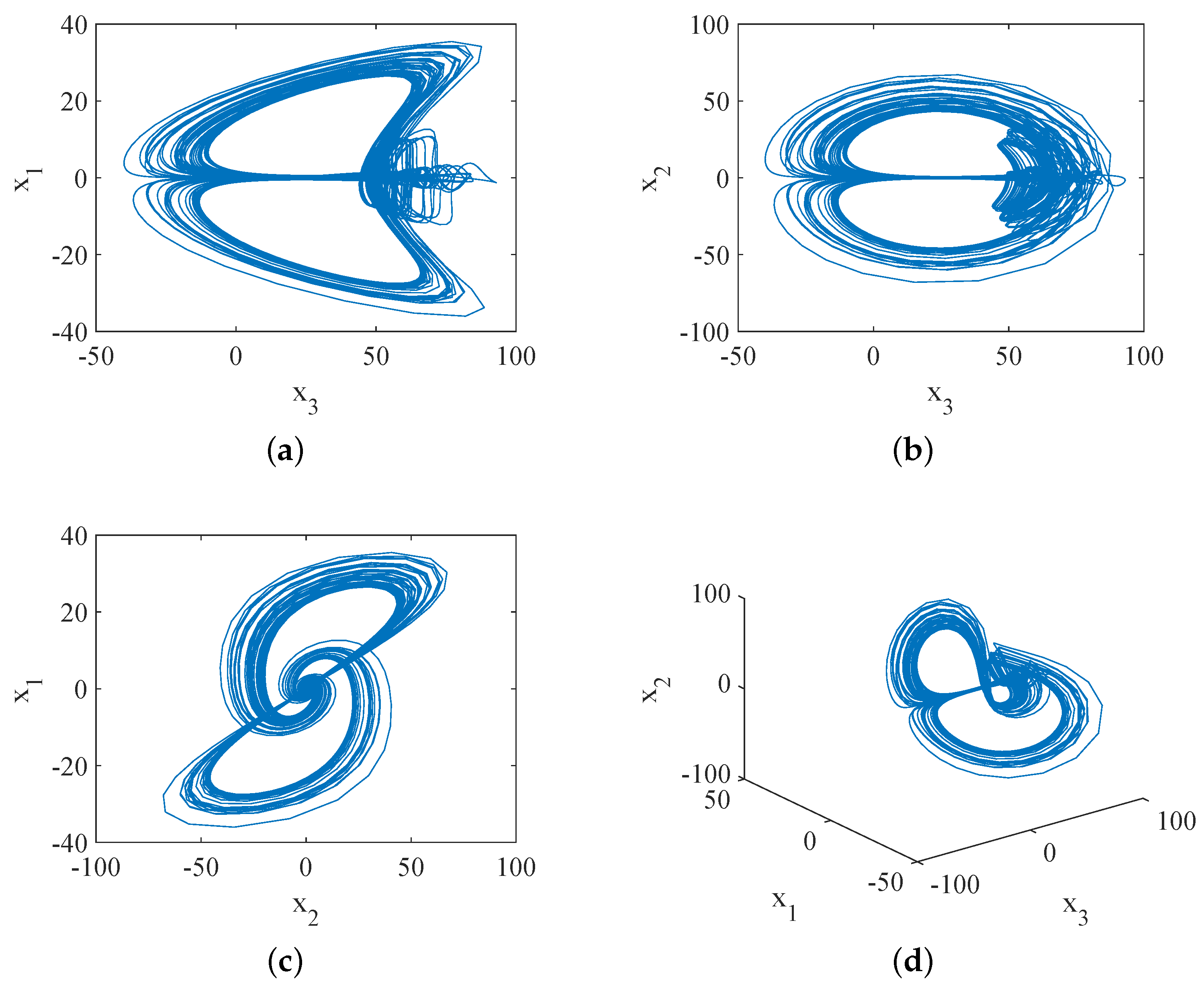
Numerical simulations were carried out to illustrate the above proposed multi-switching combination synchronization scheme. We used the same systems as in [32] with time-delays, which are fractional-order delayed Lorenz, Chen, and Rössler systems, and the numerical simulations were carried out in MATLAB.
The fractional-order delayed Lorenz system [37] was considered as the first drive system
The system in Equation (24) exhibits a chaotic attractor, as illustrated in Figure 1. The system in Equation (24) can be rewritten as
where
The fractional-order delayed Chen system [14] is the second drive system
The system in Equation (27) displays a chaotic attractor, as shown in Figure 2. We rewrite the system in Equation (27) as
where
The fractional-order delayed Rössler system is the response system, given by
where and are determined afterwards. Without the controllers, the system in Equation (30) exhibits a chaotic attractor, as illustrated in Figure 3. The system in Equation (30) is rewritten as
where
For the systems in Equations (24), (27) and (30), there are eight possible switch combination synchronization cases.
When , we have and .
When , we have and .
When , we have and .
When , we have and .
We randomly pick two cases
and
In the following, we analyze these two cases in detail.
Case 1
Here, we obtain the following results.
Theorem 2.
Supposing and or , we have the following results.
Corollary 2.
Corollary 3.
Supposing that , and , the system in Equation (30) can be stabilized to its equilibrium with the following controllers
Case 2
Here, we have the following similar results.
Theorem 3.
Corollary 4.
Corollary 5.
Supposing that , and , the system in Equation (30) can be stabilized to its equilibrium with the following controllers
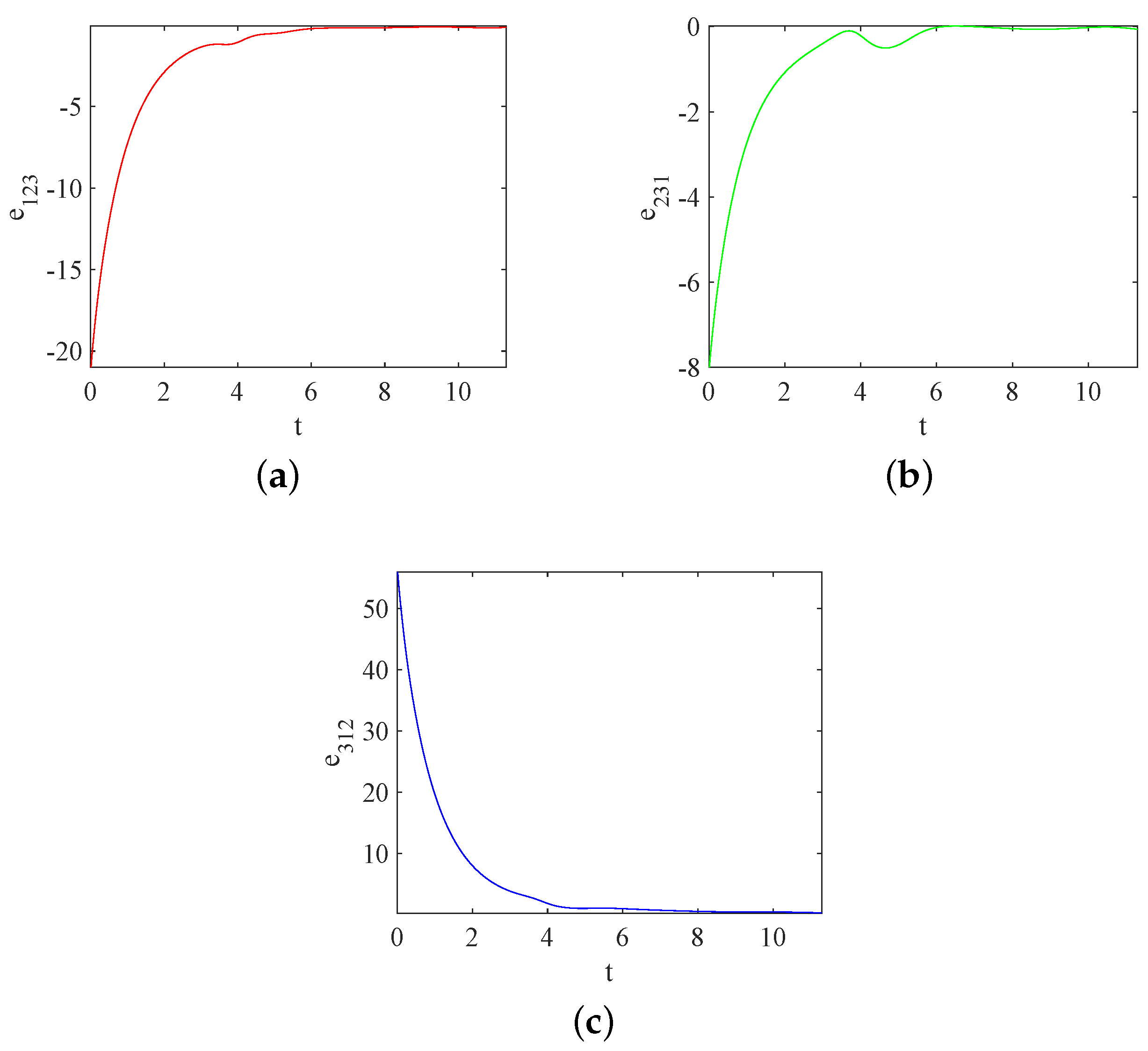
The system parameters are given as , thus the systems in Equations (24), (27) and (30) exhibit chaotic behaviors, respectively. We assume , and , and the initial values are and , respectively. Multi-switching combination synchronization between the systems in Equations (24), (27) and (30) can be realized with . Figure 4 illustrates synchronization errors , , . Figure 5 shows synchronization states vs. , vs. and vs. of the drive systems in Equations (24) and (27) and the response system in Equation (30). Figure 6 displays synchronization errors , , and . Figure 7 illustrates synchronization states vs. , vs. and vs. of the drive systems in Equations (24) and (27) and the response system in Equation (30). In Figure 4, Figure 5, Figure 6 and Figure 7, we can see that the multi-switching combination synchronization errors converge to zero, i.e., the multi-switching combination synchronizations for Cases 1 and 2 are achieved, respectively.
The feedback gain matrix K is an important factor to affect the convergence of the error systems. With the increase of the absolute value of , the convergence time will be shortened. Thus, we carried out one more simulation with . Figure 8 and Figure 9 illustrate the synchronization errors for Cases 1 and 2, respectively. By comparing Figure 4 and Figure 8, as well as Figure 6 and Figure 9, it is easy to see that convergence times are shortened obviously.
5. Conclusions
We extended previous work [32] to investigate multi-switching combination synchronization among three non-identical fractional-order delayed systems by introducing time-delays. Based on the stability theory for linear fractional-order systems with multiple time-delays, we designed appropriate controllers to obtain multi-switching combination synchronization among three non-identical fractional-order delayed systems. The simulations are in accordance with the theoretical analysis.
On the one hand, when applying multi-switching combination synchronization of fractional-order delayed chaotic systems in secure communications, fractional-order and time-delay can enrich systems’ dynamics. On the other hand, the origin information can be separated into two parts and embedded different parts in separate drive systems via combination synchronization scheme. Besides, because the switched states are unpredictable, this synchronization scheme can increase the security of the transmitted information in secure communication. Thus, the communication security will be enhanced, which makes multi-switching combination synchronization of fractional-order delayed chaotic systems able to find better applications in security communication.
Author Contributions
Methodology, X.Z.; Writing—Original Draft Preparation, B.L.; Writing—Review and Editing, Y.W.; and Funding Acquisition, X.Z.
Funding
This work was supported by the Natural Science Foundations of China under Grant No. 61463050, the NSF of Yunnan Province under Grant No. 2015FB113.
Acknowledgments
The authors sincerely thank the anonymous reviewers for their constructive comments and insightful suggestions.
Conflicts of Interest
The authors declare no conflict of interest.
References
- Mandelbrot, B.B. The Fractal Geometry of Nature; WH Freeman: New York, NY, USA, 1983; Volume 173. [Google Scholar]
- Boukal, Y.; Darouach, M.; Zasadzinski, M.; Radhy, N.E. Large-scale fractional-order systems: Stability analysis and their decentralised functional observers design. IET Control. Theory Appl. 2017, 12, 359–367. [Google Scholar] [CrossRef]
- Caponetto, R. Fractional Order Systems: Modeling and Control Applications; World Scientific: Singapore, 2010; Volume 72. [Google Scholar]
- Azar, A.T.; Vaidyanathan, S.; Ouannas, A. Fractional Order Control and Synchronization of Chaotic Systems; Springer: Berlin/Heidelberg, Germany, 2017; Volume 688. [Google Scholar]
- Fahim, S.M.; Ahmed, S.; Imtiaz, S.A. Fractional order model identification using the sinusoidal input. ISA Trans. 2018, 83, 35–41. [Google Scholar] [CrossRef]
- Lin, C.; Chen, B.; Wang, Q.G. Static output feedback stabilization for fractional-order systems in TS fuzzy models. Neurocomputing 2016, 218, 354–358. [Google Scholar] [CrossRef]
- Bendoukha, S.; Ouannas, A.; Wang, X.; Khennaoui, A.A.; Pham, V.T.; Grassi, G.; Huynh, V. The Co-existence of Different Synchronization Types in Fractional-order Discrete-time Chaotic Systems with Non–identical Dimensions and Orders. Entropy 2018, 20, 710. [Google Scholar] [CrossRef]
- Liu, Z.; Xia, T.; Wang, J. Fractional two-dimensional discrete chaotic map and its applications to the information security with elliptic-curve public key cryptography. J. Vib. Control 2018, 24, 4797–4824. [Google Scholar] [CrossRef]
- Richard, J.P. Time-delay systems: An overview of some recent advances and open problems. Automatica 2003, 39, 1667–1694. [Google Scholar] [CrossRef]
- Mircea, G.; Neamtu, M.; Opriş, D. Uncertain, Stochastic and Fractional Dynamical Systems with Delay: Applications; Lambert Academic Publishing: Saarbrücken, Germany, 2011. [Google Scholar]
- Bhalekar, S.; Daftardar-Gejji, V. Fractional ordered Liu system with time-delay. Commun. Nonlinear Sci. Numer. Simul. 2010, 15, 2178–2191. [Google Scholar] [CrossRef]
- Wang, Z.; Huang, X.; Shi, G. Analysis of nonlinear dynamics and chaos in a fractional order financial system with time delay. Comput. Math. Appl. 2011, 62, 1531–1539. [Google Scholar] [CrossRef] [Green Version]
- Wang, S.; Yu, Y.; Wen, G. Hybrid projective synchronization of time-delayed fractional order chaotic systems. Nonlinear Anal. Hybrid Syst. 2014, 11, 129–138. [Google Scholar] [CrossRef]
- Daftardar-Gejji, V.; Bhalekar, S.; Gade, P. Dynamics of fractional-ordered Chen system with delay. Pramana 2012, 79, 61–69. [Google Scholar] [CrossRef]
- Song, X.; Song, S.; Li, B. Adaptive synchronization of two time-delayed fractional-order chaotic systems with different structure and different order. Optik 2016, 127, 11860–11870. [Google Scholar] [CrossRef]
- Moaddy, K. Control and stability on chaotic convection in porous media with time delayed fractional orders. Adv. Differ. Equ. 2017, 2017, 311. [Google Scholar] [CrossRef] [Green Version]
- Hu, J.B.; Zhao, L.D.; Xie, Z.G. Studying the intermittent stable theorem and the synchronization of a delayed fractional nonlinear system. Chin. Phys. B 2013, 22, 080506. [Google Scholar] [CrossRef]
- Djennoune, S.; Bettayeb, M.; Al-Saggaf, U.M. Synchronization of fractional–order discrete–time chaotic systems by an exact delayed state reconstructor: Application to secure communication. Int. J. Appl. Math. Comput. Sci. 2019, 29, 179–194. [Google Scholar] [CrossRef]
- Ding, D.; Qian, X.; Wang, N.; Liang, D. Synchronization and anti-synchronization of a fractional order delayed memristor-based chaotic system using active control. Mod. Phys. Lett. B 2018, 32, 1850142. [Google Scholar] [CrossRef]
- Velmurugan, G.; Rakkiyappan, R. Hybrid projective synchronization of fractional-order chaotic complex nonlinear systems with time delays. J. Comput. Nonlinear Dyn. 2016, 11, 031016. [Google Scholar] [CrossRef]
- He, S.; Sun, K.; Wang, H. Synchronisation of fractional-order time delayed chaotic systems with ring connection. Eur. Phys. J. Spec. Top. 2016, 225, 97–106. [Google Scholar] [CrossRef]
- Luo, R.; Wang, Y.; Deng, S. Combination synchronization of three classic chaotic systems using active backstepping design. Chaos Interdiscip. J. Nonlinear Sci. 2011, 21, 043114. [Google Scholar] [CrossRef]
- Sun, J.; Cui, G.; Wang, Y.; Shen, Y. Combination complex synchronization of three chaotic complex systems. Nonlinear Dyn. 2015, 79, 953–965. [Google Scholar] [CrossRef]
- Xi, H.; Li, Y.; Huang, X. Adaptive function projective combination synchronization of three different fractional-order chaotic systems. Optik 2015, 126, 5346–5349. [Google Scholar] [CrossRef]
- Zhou, X.; Jiang, M.; Huang, Y. Combination synchronization of three identical or different nonlinear complex hyperchaotic systems. Entropy 2013, 15, 3746–3761. [Google Scholar] [CrossRef]
- Jiang, C.; Liu, S.; Wang, D. Generalized combination complex synchronization for fractional-order chaotic complex systems. Entropy 2015, 17, 5199–5217. [Google Scholar] [CrossRef]
- Vincent, U.E.; Saseyi, A.; McClintock, P.V. Multi-switching combination synchronization of chaotic systems. Nonlinear Dyn. 2015, 80, 845–854. [Google Scholar] [CrossRef] [Green Version]
- Zheng, S. Multi-switching combination synchronization of three different chaotic systems via nonlinear control. Optik 2016, 127, 10247–10258. [Google Scholar] [CrossRef]
- Khan, A.; Khattar, D.; Prajapati, N. Adaptive multi switching combination synchronization of chaotic systems with unknown parameters. Int. J. Dyn. Control 2018, 6, 621–629. [Google Scholar] [CrossRef]
- Ahmad, I.; Shafiq, M.; Al-Sawalha, M.M. Globally exponential multi switching-combination synchronization control of chaotic systems for secure communications. Chin. J. Phys. 2018, 56, 974–987. [Google Scholar] [CrossRef]
- Hammami, S. Multi-switching combination synchronization of discrete-time hyperchaotic systems for encrypted audio communication. IMA J. Math. Control. Inf. 2018, 36, 583–602. [Google Scholar] [CrossRef]
- Bhat, M.A.; Khan, A. Multi-switching combination synchronization of different fractional-order non-linear dynamical systems. Int. J. Model. Simul. 2018, 38, 254–261. [Google Scholar] [CrossRef]
- Khan, A.; Bhat, M.A. Multi-switching combination–combination synchronization of non-identical fractional-order chaotic systems. Math. Methods Appl. Sci. 2017, 40, 5654–5667. [Google Scholar] [CrossRef]
- Podlubny, I. Fractional Differential Equations: An Introduction to Fractional Derivatives, Fractional Differential Equations, to Methods of Their Solution and Some of Their Applications; Elsevier: Amsterdam, The Netherlands, 1998; Volume 198. [Google Scholar]
- Kvitsinskii, A. Fractional integrals and derivatives: Theory and applications. Teor. Mater. Fiz. 1993, 3, 397–414. [Google Scholar]
- Deng, W.; Li, C.; Lü, J. Stability analysis of linear fractional differential system with multiple time delays. Nonlinear Dyn. 2007, 48, 409–416. [Google Scholar] [CrossRef]
- Tang, J. Synchronization of different fractional order time-delay chaotic systems using active control. Math. Probl. Eng. 2014, 2014, 262151. [Google Scholar] [CrossRef]
Figure 1.
Chaotic attractor of Lorenz system with : (a) plane; (b) plane; (c) plane; and (d) space.

Figure 2.
Chaotic attractor of Chen system with : (a) plane; (b) plane; (c) plane; and (d) space.

Figure 3.
Chaotic attractor of Rössler system with : (a) plane; (b) plane; (c) plane; and (d) space.
Figure 3.
Chaotic attractor of Rössler system with : (a) plane; (b) plane; (c) plane; and (d) space.

Figure 4.
Synchronization errors among the systems in Equations (24), (27) and (30) with : (a) ; (b) ; and (c) .

Figure 5.
Responses for states between the systems in Equations (24) and (27) and the system in Equation (30): (a) vs. ; (b) vs. ; and (c) vs. .

Figure 6.
Synchronization errors among the systems in Equations (24), (27) and (30) with : (a) ; (b) ; and (c) .

Figure 7.
Responses for states between the systems in Equations (24) and (27) and the system in Equation (30): (a) vs. ; (b) vs. ; and (c) vs. .

Figure 8.
Synchronization errors among the systems in Equations (24), (27) and (30) with : (a) ; (b) ; and (c) .


© 2019 by the authors. Licensee MDPI, Basel, Switzerland. This article is an open access article distributed under the terms and conditions of the Creative Commons Attribution (CC BY) license (http://creativecommons.org/licenses/by/4.0/).
Share and Cite
MDPI and ACS Style
Li, B.; Wang, Y.; Zhou, X. Multi-Switching Combination Synchronization of Three Fractional-Order Delayed Systems. Appl. Sci. 2019, 9, 4348. https://0-doi-org.brum.beds.ac.uk/10.3390/app9204348
AMA Style
Li B, Wang Y, Zhou X. Multi-Switching Combination Synchronization of Three Fractional-Order Delayed Systems. Applied Sciences. 2019; 9(20):4348. https://0-doi-org.brum.beds.ac.uk/10.3390/app9204348
Chicago/Turabian StyleLi, Bo, Yun Wang, and Xiaobing Zhou. 2019. "Multi-Switching Combination Synchronization of Three Fractional-Order Delayed Systems" Applied Sciences 9, no. 20: 4348. https://0-doi-org.brum.beds.ac.uk/10.3390/app9204348
Note that from the first issue of 2016, this journal uses article numbers instead of page numbers. See further details here.