A High-Accuracy Model Average Ensemble of Convolutional Neural Networks for Classification of Cloud Image Patches on Small Datasets


Department of Computer Engineering, Hanbat National University, Daejeon 34158, Korea
*
Author to whom correspondence should be addressed.
Appl. Sci. 2019, 9(21), 4500; https://0-doi-org.brum.beds.ac.uk/10.3390/app9214500
Submission received: 11 September 2019
/
Revised: 20 October 2019
/
Accepted: 21 October 2019
/
Published: 23 October 2019
(This article belongs to the Special Issue Machine Learning Techniques Applied to Geospatial Big Data)
Abstract
:Research on clouds has an enormous influence on sky sciences and related applications, and cloud classification plays an essential role in it. Much research has been conducted which includes both traditional machine learning approaches and deep learning approaches. Compared with traditional machine learning approaches, deep learning approaches achieved better results. However, most deep learning models need large data to train due to the large number of parameters. Therefore, they cannot get high accuracy in case of small datasets. In this paper, we propose a complete solution for high accuracy of classification of cloud image patches on small datasets. Firstly, we designed a suitable convolutional neural network (CNN) model for small datasets. Secondly, we applied regularization techniques to increase generalization and avoid overfitting of the model. Finally, we introduce a model average ensemble to reduce the variance of prediction and increase the classification accuracy. We experiment the proposed solution on the Singapore whole-sky imaging categories (SWIMCAT) dataset, which demonstrates perfect classification accuracy for most classes and confirms the robustness of the proposed model.
1. Introduction
Clouds cover more than half of the globe surface. Most cloud-related research, such as climate modeling, weather forecasting, meteorology study, solar energy research, and satellite communication [1,2,3,4,5], need to analyze cloud characteristics, in which cloud categorization plays an essential role. At present, professional observers categorize cloud types; it is a time-consuming task, and some problems cannot be well handled by human observers [6]; therefore, automatic classification of clouds is a much-needed task.
Much research has been conducted on this topic. Similar with all other image classification tasks, there are two main types of feature representation approaches for cloud image classification: hand-crafted features and deep learning features [7]. In other words, traditional machine learning approaches and deep learning approaches [8]. Firstly, we review the traditional machine learning approaches. Singh and Glennen [9] used five feature extraction methods (autocorrection, co-occurrence matrices, edge frequency, Law’s features, and primitive length) and applied the k-nearest neighbor and neural network to identify the cloud types. Calbó and Sabburg [10] applied Fourier transform, statistical measurements, and pixel computation to extract image features. Heinle et al. [11] predefined statistical features to describe color and texture, and then used a k-nearest neighbor classifier. Liu et al. [12] proposed an illumination-invariant completed local ternary pattern descriptor to deal with illumination variations. Liu et al. [13] extracted some cloud structure features from segment images and edge images and used a simple classifier, which is called the rectangle method. Liu et al. [14] developed a texture classification technique with a salient local binary pattern. Liu et al. [15] used a weighted local binary descriptor. Dev et al. [16] proposed a modified texton-based approach that integrated both color and texture information to categorize cloud image patches. Gan et al. [17] used duplex norm-bounded sparse coding to classify cloud type; they extracted local descriptors from an input cloud image and then formed a holistic representation leveraging normal-bounded sparse coding and max-pooling strategy. Luo et al. [18] combined texture feature and manifold features; the manifold features extracted on symmetric positive define (SPD) matrix space that can describe the non-Euclidean geometric characteristics of the infrared images; then, used a support vector machine (SVM) classifier. Luo et al. also [19] proposed manifold kernel sparse coding and dictionary learning with three steps: feature extraction, dictionary learning, and classification. Wang et al. [20] proposed a feature extraction method with a local binary pattern. However, most of the traditional machine learning approaches which are based on hand-crafted features rely on careful choice of features, and it is necessary to find their empirical parameters; and accurate cloud classification of these methods has not been achieved satisfactorily.
In recent times, the revolution of computing capacity has supported the development of deep learning; in particular, deep learning with convolutional neural network (CNN) has shown outstanding performance in image classification [21]. CNN models are able to extract features from the image data, so there is no need for any feature extraction method. Ye et al. [22,23] improved feature extraction using a CNN by resorting to the deep convolutional visual features and the Fisher vector and then used an SVM classifier. Shi et al. [24] proposed a CNN model to extract features using different pooling strategies and used a multi-label linear SVM classifier. Zhang et al. [25] used a trained CNN to extract local features from part summing maps based on feature maps called deep visual information for multi-view ground-based cloud recognition. Phung and Rhee [26] proposed a CNN model and some regularization methods to deal with small datasets. Zhang et al. [27] proposed a CNN model that evolved from AlexNet [21].
Generally, the deep learning approaches that used CNNs achieved better results than traditional machine learning approaches; however, most of the deep learning models need large data to train due to the large number of parameters. Therefore, they cannot get high accuracy in the case of small datasets. Phung and Rhee [26] alleviated this problem with some regularization methods. This paper proposes a complete solution to achieve high classification accuracy on cloud images in small datasets using the model average ensemble of convolutional neural networks.
The remainder of this paper is organized as follows. Section 2 presents the methodology of the proposed approach. Section 3 describes the Singapore whole-sky imaging categories (SWIMCAT) dataset and presents experiments; to evaluate our proposed model, we applied K-fold cross-validation. We employ three metrics to measure performance: accuracy, F1 score, and Cohen’s kappa coefficient. To have a look inside our model, network visualization with learned convolutional filters and feature map are also illustrated. The discussions of the experiment results are presented in Section 4, and finally, the conclusion is summarized in Section 5.
2. Methodology
2.1. CNN Model Design
In deep learning, CNNs are the most common networks used with image classification. CNNs were inspired by the human visual system proposed by Fukushima [28] and LeCun et al. [29]. They are state-of-the-art approaches for pattern recognition, object detection, and many other image applications. In particular, in 2012, the champion of the ImageNet Large Scale Visual Recognition Challenge 2012 competition [30,31] was a deep CNN solution by Krizhevsky et al. [21] which demonstrated the great power of deep CNNs.
CNNs are very different from other pattern recognition algorithms in that CNNs combine both feature extraction and classification [32]. Figure 1 shows an example of a simple schematic representation of a basic CNN. This simple network consists of five different layers: an input layer, a convolution layer, a pooling layer, a fully-connected layer, and an output layer. These layers are divided into two parts: feature extraction and classification. Feature extraction consists of an input layer, a convolution layer, and a pooling layer, while classification consists of a fully-connected layer and an output layer. The input layer specifies a fixed size for the input images, which is resized if needed. Then the image is convolved with multiple learned kernels using shared weights by convolution layer. Next, the pooling layer reduces the image size while trying to maintain the contained information. The outputs of the feature extraction are known as feature maps. The classification combines the extracted features in the fully-connected layers. Finally, there exists one output neuron for each object category in the output layer. The output of the classification part is the classification result.
In real applications, the feature extraction part contains many convolution and pooling layers, and the classification part also contains many fully connected layers. Common CNN architectures have the following pattern [33]:
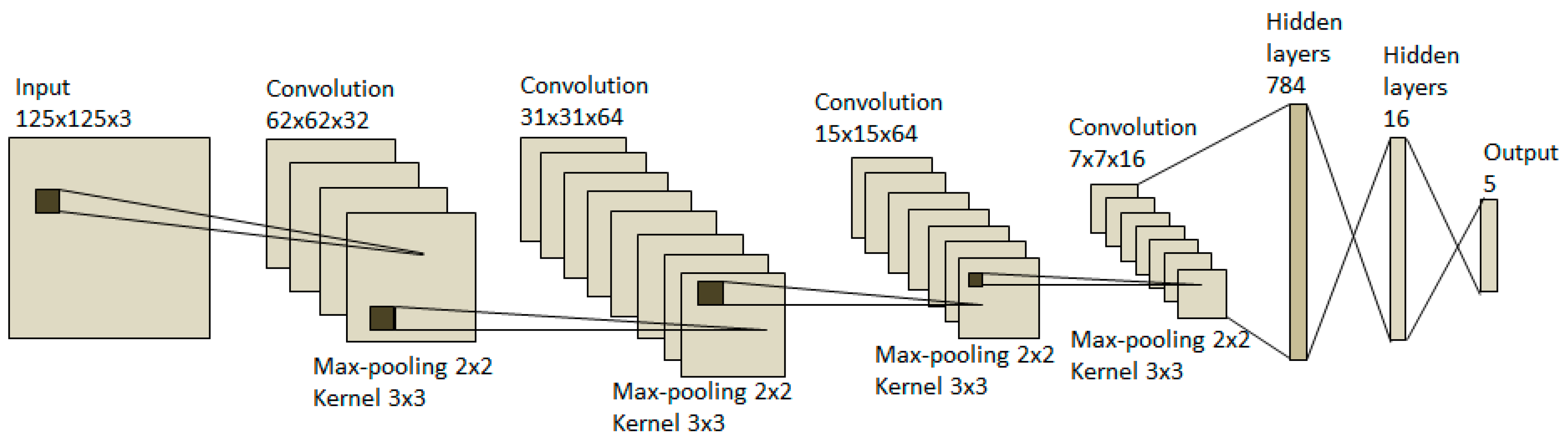
where IN denotes the input layer, CONV denotes the convolution layer, POOL denotes the pooling layer, FC denotes the fully connected layer, and OUT denotes the output layer. M and N are integer numbers, “*” indicates repetition and “?” indicates optional. The activations were not mentioned, but by default the activation always follows the CONV and FC layers. In this research, we chose four blocks of CONV layers and POOL layers in the feature extraction part and three FC layers in the classification part, i.e., M = 4 and N = 3. The architecture of the proposed CNN model is shown in Figure 2.
The detailed parameters of the proposed CNN model architecture are shown in Table 1. We applied 3 × 3 kernel sizes for all CONV layers and 2 × 2 window sizes for the all POOL layers. We use 32 filters for the first CONV layer, 64 filters for the second and third CONV layers and 16 filters for the fourth CONV layer. We use 784 neurons for the first FC layer and 16 neurons for the second FC layer. We apply dropout [34] to the classification part. We specify a dropout probability of 0.25 between the first and the second FC layers, and a dropout probability of 0.5 between the second and the third FC layers.
2.2. Model Average Ensemble of CNN
Deep neural networks are nonlinear models that learn via a stochastic training mechanism, so they are highly flexible and capable of learning complex relationships between variables and approximating any mapping function for given training data. A drawback of this flexibility is that they are sensitive to the specifics of the training data and random initialization. They may produce a different set of weights each time they are trained. This is especially true with small datasets. The models with these different weights produce different predictions. In other words, neural networks have a high variance. A successful approach to overcome the high variance problem is ensemble learning [35,36].
In this research, we apply a model average ensemble to the designed CNN model in Section 2.1. The model average ensemble of neural networks is shown in Figure 3. It consists of multiple neural network models, and each model is trained with the same image data but different random initialization. When classifying an input image, the image is passed to each network, and it classifies the image independently. Final prediction is obtained by the combination of all the predictions from these models by averaging.
We use model averaging to reduce the variance of the model, reduce the generalization error of the model, and achieve higher accuracy than any single model. In this study, we propose an ensemble of CNNs that includes 10 individual CNNs with the same model architecture. In each CNN model, we used the model design described in the previous section, whose detailed information is shown in Table 1.
2.3. Model Regularization
One of the most challenging problems in designing machine learning models is how to make sure that the model will perform well not only on the training data, but also on new inputs. Two common ways to overcome this problem are collecting more data and applying regularization. During the design stage of our CNN model in Section 2.1, the dropout technique was introduced as a regularization technique that works by modifying the network architecture. However, in this study, only a small dataset is available, so more regularization is needed. We used two more regularization methods, namely, L2 weight regularization and data augmentation.
2.3.1. L2 Weight Regularization
A common way to mitigate overfitting is to put constraints on the complexity of a network by forcing its weights to take only small values, which makes the distribution of weight values more regular. It is done by adding to the loss function of the network a cost associated with having large weights. In this study, we apply L2 regularization with L2 = 0.0002.
2.3.2. Data Augmentation
Data augmentation is a regularization method that generates more training data from the original data. It is performed by applying random geometric transforms such that the class labels are not changed. In this study, we applied data augmentation similar to that by Phung and Rhee [26]. The detailed parameters of each augmentation are shown in Table 2. We choose a rotation range of 40 degrees, and a translation range of 20% for both vertical and horizontal. We also choose shear transformation and zoom transformation with the range of 20%. Finally, a horizontal flip and a vertical flip are applied as well. We only perform augmentation during the training and do not perform augmentation during the validation and testing.
3. Experiments
3.1. SWIMCAT Dataset
Although there is much research in this area, the public database in this area is very rare. Recently, Dev et al. [16] introduced a database called Singapore Whole-Sky Imaging CATegories (SWIMCAT). The images were captured in Singapore using the Wide Angle High-Resolution Sky Imaging System (WAHRSIS) and a calibrated ground-based whole sky imager [37].
As specified in Table 3, the dataset has 784 images, which are categorized into five distinct categories. They are clear sky, patterned clouds, thick dark clouds, thick white clouds, and veil clouds. All images have the dimension of 125 × 125 pixels. These categories are defined based on the basics of visual characteristics of sky and cloud conditions and consultation with experts from the Singapore Meteorological Services [16,37]. Figure 4 shows some random images of each class from the SWIMCAT dataset in rows.
3.2. Experimental Configuration
The configuration used for these experiments:
CPU: Intel core i5-7500 (3.40 GHz);
Memory: 16 GB DDR4;
GPU: NVIDA GetFore GTX-1060 6 GB memory;
The software used is the following:
Window 10 professional;
Anaconda IDE with Python 3.6;
All of our experiments are conducted using the Keras deep learning library [38] with a TensorFlow [39] back-end, a powerful framework for deep learning. We conduct the experiment by creating an ensemble model from 10 single models. We trained the proposed network using the Adam optimizer [40] with learning rate of 0.0001, a batch size of eight images, and we trained for 1000 epochs. The best model configuration as evaluated by the loss of the test set is chosen.
3.3. K-Fold Cross-Validation
To evaluate our proposed model, we applied K-fold cross-validation. We randomly split the data into five partitions of equal size (k = 5). For each partition n, we trained the proposed model on the remaining four partitions, and tested it on partition n. The final score was the average of all five scores obtained. The schematic of K-fold validation is shown in Figure 5.
3.4. Performance Metrics
In this work, we consider the following performance measures: accuracy (A), F1 score (F1), and Cohen’s kappa coefficient (K) to measure performance. True positives (tp), true negatives (tn), false positive (fp), and false negative (fn) are used to calculate accuracy and F1 score. The calculations are as follows.
• Accuracy
The accuracy performs evaluation of the classification algorithm. It is defined as:
where is the number of tp for class c, C is the number of classes, and N is total number of instances.
• F1 score
F1 score is a measure of test’s accuracy that considers both the precision and recall of the test to compute the score. It is given by the formula [41]:
• Cohen’s kappa
Cohen’s kappa measures the degree of agreement, or disagreement between two people observing the same phenomenon [42]. In our experiment, we calculated Cohen’s kappa from the confusion matrix [43]:
where represent the diagonal elements of the confusion matrix, where represent the total actual instances of class Ci, and represent the total predicted instances of class Ci, and N is total number of instances in the test set.
3.5. Network Visualization
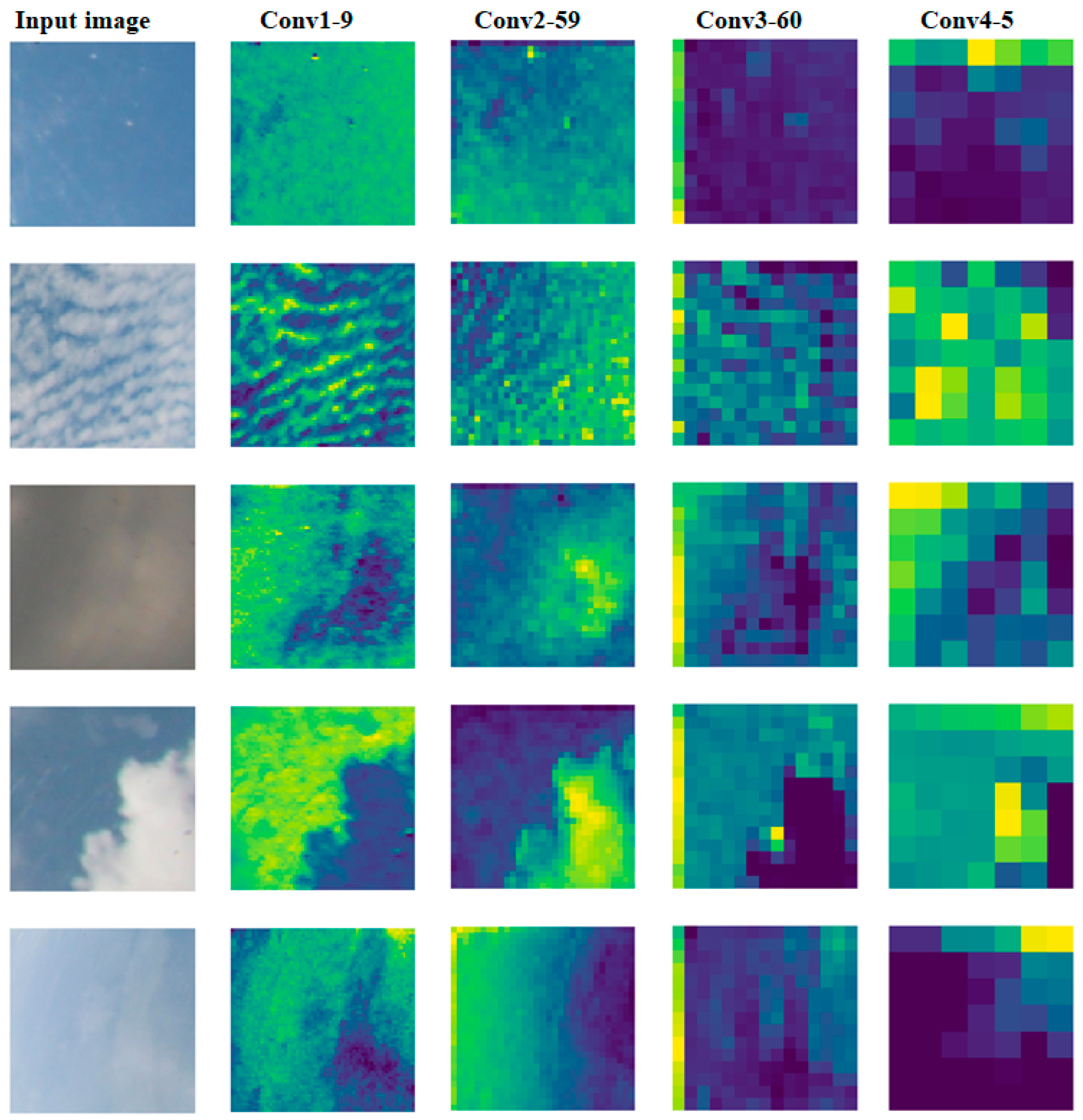
To have a better understanding of how the proposed network performs, we show both the learned convolutional filters and feature maps of the proposed model. The learned filters display visual patterns for each layer. To demonstrate these visual patterns, we used image size 125 × 125 for both input image and output image. They are shown in Figure 6 where CONV1, CONV2, CONV3, and CONV4 are immediate layers no. 2, 5, 8, and 11 in Table 1, respectively. The filters from the first layer show simple textures and colors, the deeper layers resemble textures found in the raw images. The feature map visualization of each layer is seen in Figure 7. The shallow layers tend to capture the texture information, and the deeper layers reflect the high-level semantic characteristics. The CONV1 layer (the shallow layer) clearly visualizes the original shape of different clouds. The CONV4 layer (deep layer) loses the detail information but it visualizes the edges of different clouds.
4. Results and Discussion
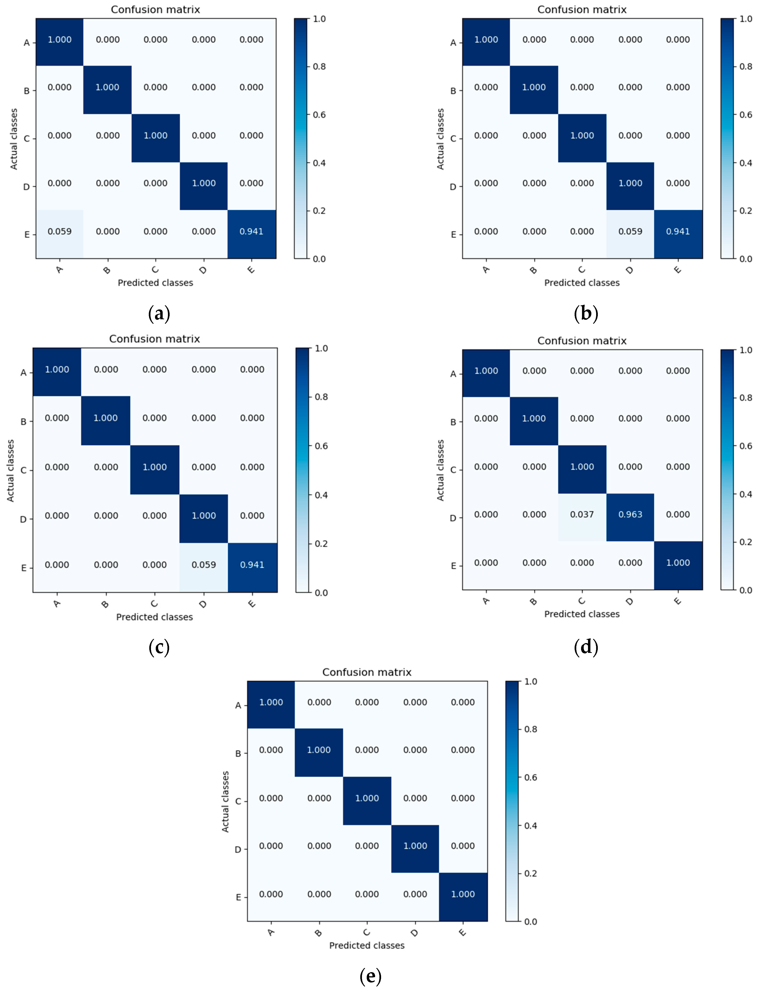
We performed our experiments with the configuration described in the previous section. We describe the performance of our model in confusion matrixes; five confusion matrixes for five folds are shown in Figure 8. In each confusion matrix, each column represents the instances in a predicted class, and each row represents the instances in the actual class. Values on the matrix diagonal indicate correct prediction, and the values outside the matrix diagonal show incorrect prediction. A summary of the experimental results is given in Table 4. We obtained an average accuracy of 99.5%. In all five folds, a classification accuracy of 100% was achieved for the sky, patterned clouds, and thick dark cloud classes. Fold 5 achieved an accuracy of 100% for all classes.
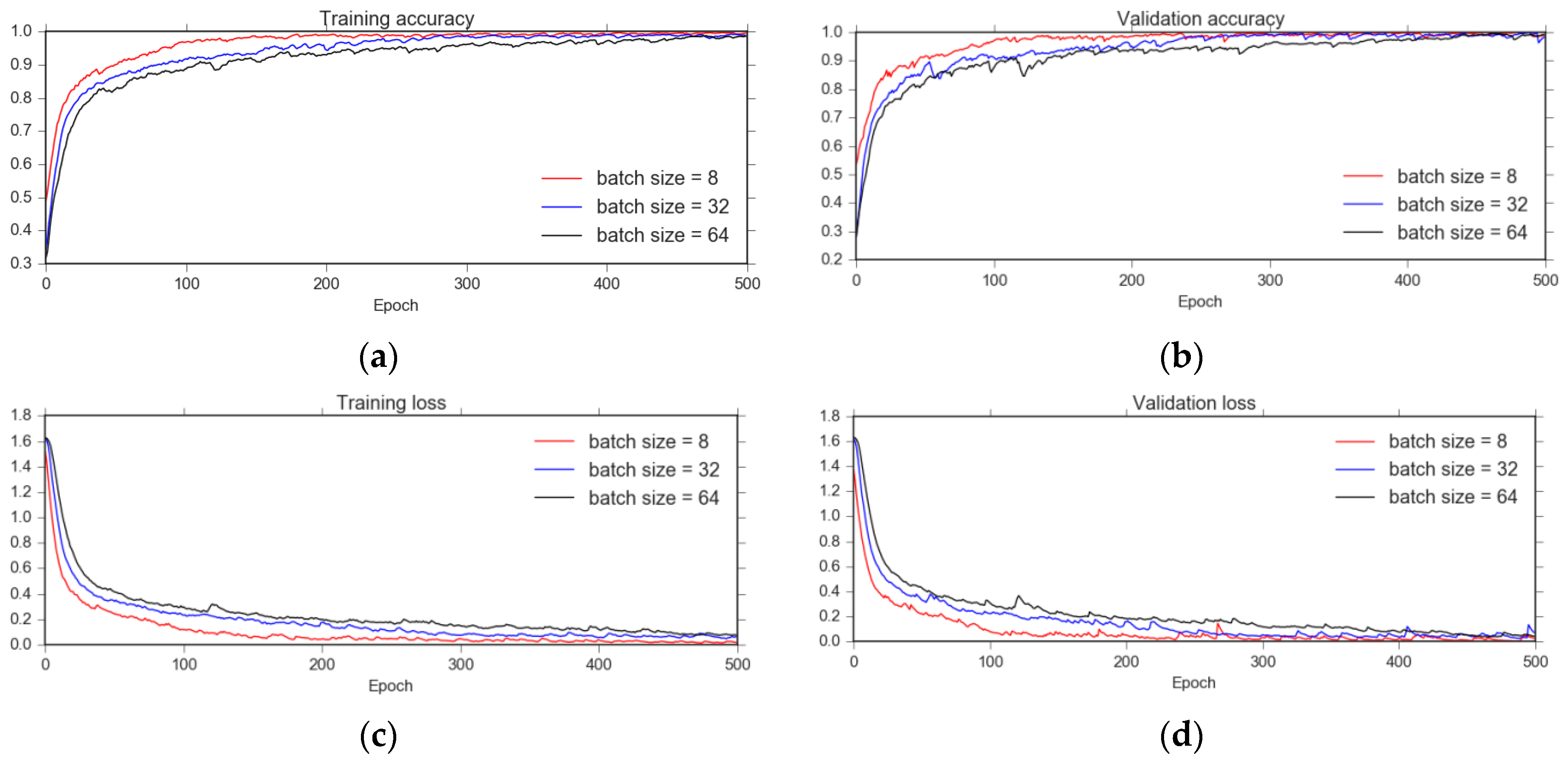
Here we discuss the effect of some parameters on the proposed model during the training, and we compare our results to the previous methods. Two hyper-parameters are considered in our experiments: the learning rate of the optimizer and the batch size. The effect of the number of models in the ensemble is also discussed. One of the most important hyper-parameters of neural networks is the learning rate, which controls how quickly a neural network model learns a problem; Figure 9 shows the effect of learning rate parameters on training and validation history. With a learning rate of 0.001, oscillating problems still occur in both training and validation curves. The reason is that this learning rate is still large, it is possible to make large weights, and then cause oscillation. In Figure 9, the oscillation is seen clearly at the 415th epoch. However, when we reduce the learning rate from 0.001 to a rate of 0.0001, the performance of both the training and the validation improve significantly and are very stable. Figure 10 demonstrates the effect of batch size on the training and validation history. With a big batch size, such as the batch size of 64, there are some small oscillating problems in the early epochs, and after a long time of training, these oscillations are eliminated. With a small batch size, such as the batch size of eight, the training process is smooth and converges faster. In summary, a smaller batch size produces a faster training process, but it does not have much effect on the accuracy.
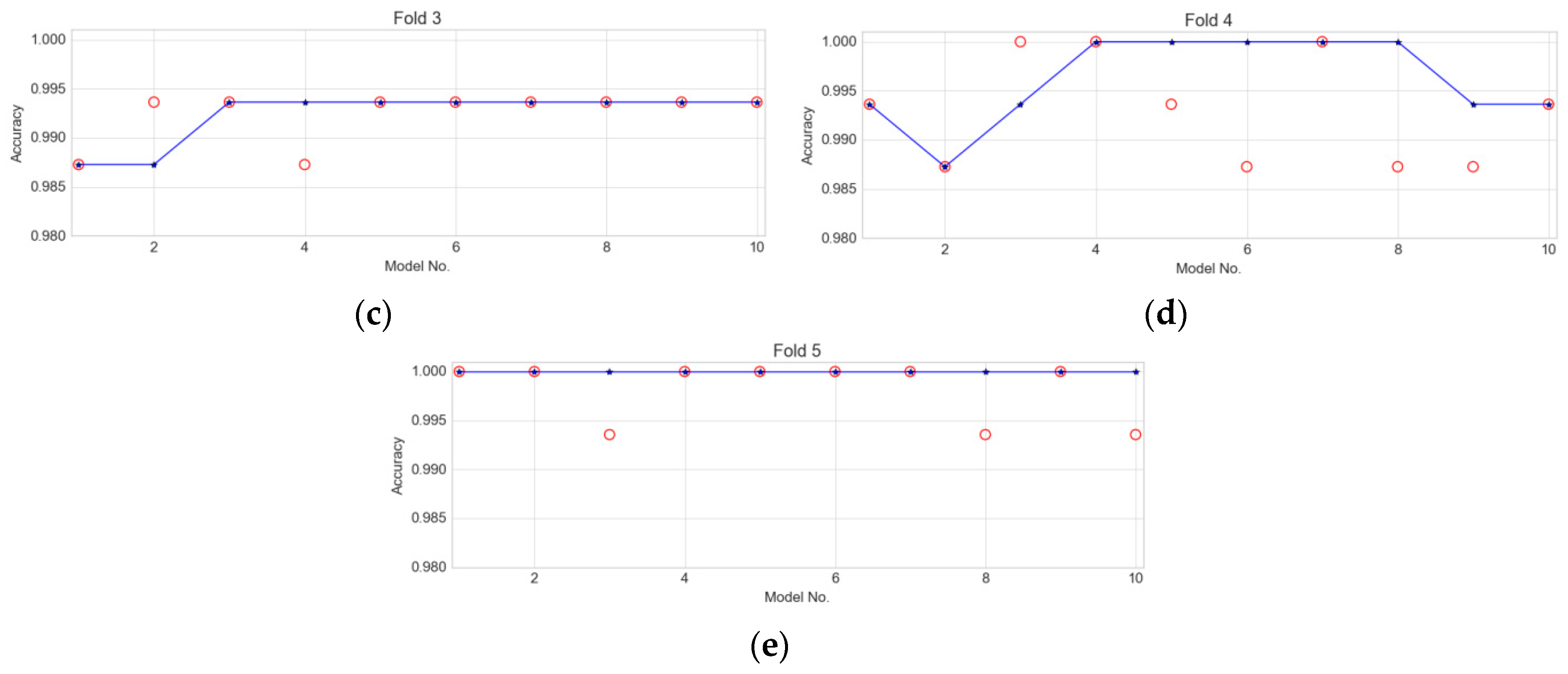
To evaluate the effect of the number of models in the ensemble, we created different ensembles with the number of models ranging from one to ten and evaluated the performance of each ensemble on the test set. We also evaluated the performance of each of the ten standalone models on the test set. Figure 11 shows the accuracies of the accumulative ensemble models indicated by the blue stars and curve as well as the accuracies of the unique standalone models indicated by the red circles. When there is one model, the results of the ensemble model and the single model are always identical, and as the size of the model increases, the advantages of the ensemble are clearly revealed. The traditional ensemble method, such as random forests [44,45], typically consists of 30 decision trees, and in many cases the number of decision trees is over 100. However, the number of models in a CNN ensemble is normally from 5 to 10 because more models make it more time consuming and computationally expensive to train. As shown in Figure 11, when there are five or more models, the blue curves of the ensembles showed accuracies that are better or comparable to those of single models in almost all cases. Fold 1, fold 2, and fold 5 had the same characteristics. The use of an ensemble helps to achieve high accuracies and keep accuracies stabilized better than randomly selected single models whose accuracies are sometimes high and sometimes a little lower. In fold 3, increasing the model number of the ensemble does not only increase accuracy, but it also maintains a stable state. In the case of fold 4, when the number of models in the ensemble increased, the accuracy also is increased; however, many single models with lower accuracies added make the accuracy of the ensemble models a little lower. Nonetheless, the ensemble accuracy is still higher than almost any randomly selected single models.
Table 5 reports the comparison of the accuracy, F1 score, and Cohen’s kappa of our approach and other methods. In this study, we compare our experimental result with all other previous studies that experimented with the same dataset (SWIMCAT). The performance metrics are calculated using confusion matrix data that were published in previous research (in the case of Shi et al. [24], the detail confusion matrix data was not provided; only accuracy is compared). The first three papers [20], [16], and [19] applied traditional machine learning approaches and they obtained accuracies of 91.1%, 95.1%, and 98.3%, respectively. The other papers [26], [27], and [24] applied deep learning with CNN approaches. These deep learning approaches got better results than the traditional machine learning ones, achieving accuracies of 98.6%~98.7%. Along with accuracy, the F1 score and the Cohen’s kappa of the deep learning approaches are also better than the traditional machine learning approaches. Our proposed method is an optimized CNN model with regularization techniques and involves the ensemble method. The accuracy of our model is greater than that of all other methods and it reaches an almost perfect accuracy of 99.5%, both F1 score and Cohen’s kappa got 0.993.
5. Conclusions
This paper presents an ensemble of convolutional neural networks for classification of cloud image patches on small datasets. We designed a CNN model with a suitable number of convolutional layers and fully connected layers for small datasets. The central problem of small datasets is overfitting, for which we applied two regularization techniques—L2 weight regularization and data augmentation—to avoid overfitting and to increase generalization of the model. To further improve the classification performance, we applied a model average ensemble, which separately trained several different models with the same architecture and then combined their predictions for testing. The reason why the model average ensemble works so well is that different CNN models will usually not make all the same errors on the test set. The difference in errors will be more in the case of small datasets, so different models compensate for errors of the other ones. Therefore, a model average ensemble of CNN models performs better than any random selected model of its members. We experimented with SWIMCAT, which is a small dataset with only 784 images. The small dataset is also sensitive to the specifics of the training data and random initialization. To ensure that the proposed model is robust, we applied k-fold cross-validation in the experiments, and employed F1 score and Cohen’s kappa coefficient for performance evaluation. The results of all the experiments showed very high classification accuracy. With a minimum accuracy of 99.4% and maximum accuracy of 100%, the overall average accuracy of our model was 99.5%. Both F1 score and Cohen’s kappa coefficient are 0.993. The results prove that the proposed model not only achieves a high accuracy but is also robust. Compared with all other previous methods, the proposed method achieved the best results.
Author Contributions
Conceptualization, V.H.P.; Methodology, V.H.P.; Project administration, E.J.R.; Resources, E.J.R.; Writing-original draft, V.H.P.; Writing-review & editing, V.H.P. and E.J.R.
Funding
This research received no external funding.
Conflicts of Interest
The authors declare no conflict of interest.
Abbreviations
The following abbreviations are used in this paper:
| Abbreviations | Meaning |
| Adam | Adaptive moment estimation |
| CNN | Convolutional neural networks |
| SVM | Support Vector Machine |
| SWIMCAT | Singapore Whole-sky Imaging CATegories |
| SPD | Symmetric Positive Define |
| WAHRSIS | Wide Angle High-Resolution Sky Imaging System |
References
- Naud, C.M.; Booth, J.F.; Del Genio, A. The relationship between boundary layer stability and cloud cover in the post-cold frontal region. J. Clim. 2016, 29, 8129–8149. [Google Scholar] [CrossRef] [PubMed]
- Cui, F.; Ju, R.R.; Ding, Y.Y.; Ding, H.; Cheng, X. Prediction of regional global horizontal irradiance combining ground-based cloud observation and numerical weather prediction. Adv. Mater. Res. 2015, 1073, 388–394. [Google Scholar] [CrossRef]
- Liu, Y.; Key, J.R.; Wang, X. The influence of changes in cloud cover on recent surface temperature trends in the arctic. J. Clim. 2008, 21, 705–715. [Google Scholar] [CrossRef]
- Hartmann, D.L.; Ockert-Bell, M.E.; Michelsen, M.L. The effect of cloud type on earth’s energy balance: Global analysis. J. Clim. 1992, 5, 1281–1304. [Google Scholar] [CrossRef]
- Yuan, F.; Lee, Y.H.; Meng, Y.S. Comparison of radio-sounding profiles for cloud attenuation analysis in the tropical region. In Proceedings of the IEEE Antennas and Propagation Society International Symposium (APSURSI), Memphis, TN, USA, 6–11 July 2014. [Google Scholar] [CrossRef]
- Pagès, D.; Calbò, J.; Long, C.; González, J.; Badosa, J. Comparison of several ground-based cloud detection techniques. In Proceedings of the European Geophysical Society XXVII General Assembly, Nice, France, 21–26 April 2002. [Google Scholar]
- Hu, J.; Chen, Z.; Yang, M.; Zhang, R.; Cui, Y. A multiscale fusion convolutional neural network for Plant Leaf Recognition. IEEE Signal Process. Lett. 2018, 25, 853–857. [Google Scholar] [CrossRef]
- Wu, X.; Zhan, C.; Lai, Y.K.; Cheng, M.M.; Yang, J. IP102: A large-scale benchmark dataset for insect pest recognition. In Proceeding of the IEEE Conference on Computer Vision and Pattern Recognition, Long Beach, CA, USA, 16–20 June 2019. [Google Scholar]
- Singh, M.; Glennen, M. Automated ground-based cloud recognition. Pattern Anal. Appl. 2005, 8, 258–271. [Google Scholar] [CrossRef]
- Calbó, J.; Sabburg, J. Feature extraction from whole-sky ground-based images for cloud-type recognition. J. Atmos. Ocean. Technol. 2008, 25, 3–14. [Google Scholar] [CrossRef]
- Heinle, A.; Macke, A.; Srivastav, A. Automatic cloud classification of whole sky images. Atmos. Meas. Tech. 2010, 3, 557–567. [Google Scholar] [CrossRef] [Green Version]
- Liu, S.; Wang, C.; Xiao, B.; Zhang, Z.; Shao, Y. Illumination-invariant completed LTP descriptor for cloud classification. In Proceedings of the 5th International Congress on Image and Signal Processing, Chongqing, China, 16–18 October 2012. [Google Scholar] [CrossRef]
- Liu, L.; Sun, X.J.; Chen, F.; Zhao, S.J.; Gao, T.C. Cloud classification based on structure features on infrared images. J. Atmos. Ocean. Technol. 2011, 28, 410–497. [Google Scholar] [CrossRef]
- Liu, S.; Wang, C.; Xiao, B.; Zhang, Z.; Shao, Y. Salient local binary pattern for ground-based cloud classification. Acta Meteorol. Sin. 2013, 27, 211–220. [Google Scholar] [CrossRef]
- Liu, S.; Zhang, Z.; Mei, X. Ground-based cloud classification using weighted local binary patterns. J. Appl. Remote Sens. 2015, 9, 905062. [Google Scholar] [CrossRef]
- Dev, S.; Lee, Y.H.; Winkler, S. Categorization of cloud image patches using an improved texton-based approach. In Proceedings of the IEEE International Conference on Image Processing (ICIP), Quebec City, QC, Canada, 27–30 September 2015. [Google Scholar]
- Gan, J.R.; Lu, W.T.; Li, Q.Y.; Zhang, Z.; Yang, J.; Ma, Y.; Yao, W. Cloud type classification of total-sky images using duplex norm-bounded sparse coding. IEEE J. Sel. Top. Appl. Earth Obs. Remote Sens. 2017, 10, 3360–3372. [Google Scholar] [CrossRef]
- Luo, Q.X.; Meng, Y.; Liu, L.; Zhao, X.F.; Zhou, Z.M. Cloud classification of ground-based infrared images combining manifold and texture features. Atmos. Meas. Technol. 2018, 11, 5351–5361. [Google Scholar] [CrossRef] [Green Version]
- Luo, Q.X.; Zhou, Z.M.; Meng, Y.; Li, Q.; Li, M.Y. Ground-based cloud-type recognition using manifold kernel sparse coding and dictionary learning. Adv. Meteorol. 2018, 2018, 9684206. [Google Scholar] [CrossRef]
- Wang, Y.; Shi, C.Z.; Wang, C.H.; Xiao, B.H. Ground-based cloud classification by learning stable local binary patterns. Atmos. Res. 2018, 207, 74–89. [Google Scholar] [CrossRef]
- Krizhevsky, A.; Sutskever, I.; Hinton, G.E. ImageNet classification with deep convolutional neural networks. In Proceedings of the Neural Information Processing Systems Conference, Lake Tahoe, NV, USA, 3–6 December 2012; pp. 1097–1105. [Google Scholar]
- Ye, L.; Cao, Z.; Xiao, Y. Ground-based cloud image categorization using deep convolutional features. In Proceedings of the IEEE International Conference on Image Processing, Quèbec City, QC, Canada, 27–30 September 2015; pp. 4808–4812. [Google Scholar]
- Ye, L.; Cao, Z.; Xiao, Y.; Li, W. DeepCloud: Ground-Based Cloud Image Categorization Using Deep Convolutional Features. IEEE Trans. Geosci. Remote Sens. 2017, 55, 5729–5740. [Google Scholar] [CrossRef]
- Shi, C.; Wang, C.; Wang, Y.; Xiao, B. Deep convolutional activations-based features for ground-based classification. IEEE Geosci. Remote Sens. Lett. 2017, 14, 816–820. [Google Scholar] [CrossRef]
- Zhang, Z.; Li, D.H.; Liu, S.; Xiao, B.H.; Cao, X.Z. Multi-view ground-based cloud recognition by transferring deep visual information. Appl. Sci. 2018, 8, 748. [Google Scholar] [CrossRef]
- Phung, V.H.; Rhee, E.J. A Deep Learning Approach for Classification of Cloud Image Patches on Small Datasets. J. Inf. Commun. Converg. Eng. 2018, 16, 173–178. [Google Scholar] [CrossRef]
- Zhang, J.; Liu, P.; Zhang, F.; Song, Q. CloudNet: Ground-based cloud classification with deep convolutional neural network. Geophys. Res. Lett. 2018, 45, 8665–8672. [Google Scholar] [CrossRef]
- Fukushima, K. Neocognitron: A self-organizing neural network model for a mechanism of pattern recognition unaffected by shift in position. Biol. Cybern. 1980, 36, 193–202. [Google Scholar] [CrossRef] [PubMed]
- LeCun, Y.; Bottou, L.; Bengio, Y.; Haffner, P. Gradient-based learning applied to document recognition. Proc. IEEE 1998, 86, 2278–2324. [Google Scholar] [CrossRef] [Green Version]
- ImageNet Large Scale Visual Recognition Competition (ILSVRC). Available online: http://www.image-net.org/challenges/LSVRC/ (accessed on 10 October 2019).
- Deng, J.; Dong, W.; Socher, R.; Li, L.; Li, K.; Li, F.F. ImageNet: A Large-Scale Hierarchical Image Database. In Proceedings of the IEEE Conference on Computer Vision and Pattern Recognition (CVPR’09), Miami Beach, FL, USA, 20–25 June 2009. [Google Scholar]
- Hertel, L.; Barth, E.; Käster, T.; Martinetz, T. Deep convolutional neural networks as generic feature extractors, In Proceeding of the 2015 International Joint Conference on Neural Networks, Killarney, Ireland, 12–16 July 2015.
- CS231n Convolutional Neural Networks for Visual Recognition. Available online: http://cs231n.github.io/convolutional-networks/ (accessed on 10 October 2019).
- Srivastava, N.; Hinton, G.E.; Krizhevsky, A.; Sutskever, I.; Salakhutdinov, R. Dropout: A simple way to prevent neural networks from overfitting. J. Mach. Learn. Res. 2014, 15, 1929–1958. [Google Scholar]
- Hansen, L.K.; Salamon, P. Neural Network Ensembles. IEEE Trans. Pattern Anal. Mach. Intell. 1990, 12, 993–1001. [Google Scholar] [CrossRef]
- Krogh, A.; Vedelsby, J. Neural network ensembles, cross validation, and active learning. In Advances in Neural Information Processing Systems; MIT Press: Cambridge, MA, USA, 1995; pp. 231–238. [Google Scholar]
- Dev, S.; Savoy, F.M.; Lee, Y.H.; Winkler, S. WAHRSIS: A low-cost, high-resolution whole sky imager with ner-infrared capabilities. In Proceedings of the SPIE—The International Society for Optical Engineering, Baltimore, MD, USA, 5–9 May 2014; Volume 9071. [Google Scholar] [CrossRef]
- Keras. Available online: https://keras.io/ (accessed on 10 October 2019).
- Tensorflow. Available online: https://www.tensorflow.org/ (accessed on 10 October 2019).
- Kingma, D.P.; Ba, J.L. Adam: A Method for Stochastic Optimization. In Proceedings of the ICLR, Vancouver Convention Center, Vancouver, BC, Canada, 7–9 May 2015; pp. 1–15. [Google Scholar]
- F1 Score. Available online: https://en.wikipedia.org/wiki/F1_score (accessed on 10 October 2019).
- Cohen, J. A coefficient of agreement for nominal scales. Educ. Psychol. Meas. 1960, 20, 37–46. [Google Scholar] [CrossRef]
- Tallón-Ballesteros, A.J.; Riquelme, J.C. Data mining methods applied to a digital forensics task for supervised machine learning. In Computational Intelligence in Digital Forensics: Forensic Investigation and Applications, 1st ed.; Muda, A.K., Choo, Y.H., Abraham, A., Srihari, S.N., Eds.; Springer: Cham, Switzerland, 2014; Volume 555, pp. 413–428. [Google Scholar]
- Hastie, T.; Friedman, J.; Tibshirani, R. Ensemble Learning. In The Elements of Statistical Learning: Data Mining, Inference, and Prediction, 2nd ed.; Springer: New York, NY, USA, 2009; pp. 605–624. [Google Scholar]
- Breiman, L. Random Forests. Mach. Learn. 2001, 45, 5–32. [Google Scholar] [CrossRef] [Green Version]
Figure 1.
Schematic diagram of a basic convolutional neural network (CNN) architecture [26].
Figure 1.
Schematic diagram of a basic convolutional neural network (CNN) architecture [26].

Figure 2.
The proposed CNN model architecture.

Figure 3.
An ensemble of neural networks.

Figure 4.
Sample images from the Singapore whole-sky imaging categories (SWIMCAT) dataset.

Figure 5.
Schematic of K-fold cross-validation.

Figure 6.
Visualizing learned convolutional filters: (a) Convolutional filters of CONV1; (b) Convolutional filters of CONV2; (c) Convolutional filters of CONV3; (d) Convolutional filters of CONV4.
Figure 6.
Visualizing learned convolutional filters: (a) Convolutional filters of CONV1; (b) Convolutional filters of CONV2; (c) Convolutional filters of CONV3; (d) Convolutional filters of CONV4.


Figure 7.
Visualization of feature maps from four CONV blocks (denoted CONV1-9: channel number 9 on CONV block 1).
Figure 7.
Visualization of feature maps from four CONV blocks (denoted CONV1-9: channel number 9 on CONV block 1).

Figure 8.
Fold cross validation results expressed in confusion matrixes: (a) Confusion matrix showing results of test on fold 1; (b) Confusion matrix showing results of test on fold 2; (c) Confusion matrix showing results of test of fold 3; (d) Confusion matrix showing results of test on fold 4; (e) Confusion matrix showing results of test on fold 5.

Figure 9.
Effect of learning rate: (a) Training accuracy plot; (b) Validation accuracy plot; (c) Training loss plot; (d) Validation loss plot.
Figure 9.
Effect of learning rate: (a) Training accuracy plot; (b) Validation accuracy plot; (c) Training loss plot; (d) Validation loss plot.

Figure 10.
Effect of batch size: (a) Training accuracy plot; (b) Validation accuracy plot; (c) Training loss plot; (d) Validation loss plot.
Figure 10.
Effect of batch size: (a) Training accuracy plot; (b) Validation accuracy plot; (c) Training loss plot; (d) Validation loss plot.

Figure 11.
Accuracy of the ensemble model vs. single model. The red circles show accuracy of the single models and the blue stars and curve show accuracy of the ensemble model: (a) Fold 1; (b) Fold 2; (c) Fold 3; (d) Fold 4; (e) Fold 5.
Figure 11.
Accuracy of the ensemble model vs. single model. The red circles show accuracy of the single models and the blue stars and curve show accuracy of the ensemble model: (a) Fold 1; (b) Fold 2; (c) Fold 3; (d) Fold 4; (e) Fold 5.


Table 1.
Detailed parameters of the designed model.
| No. | Layer | Output Size | Filter Size | Stride Size | Dropout |
|---|---|---|---|---|---|
| 1. | Input | 125 × 125 × 3 | - | - | - |
| 2. | Convolution 1 | 125 × 125 × 32 | 3 × 3 | - | - |
| 3. | Relu | 125 × 125 × 32 | - | - | - |
| 4. | Max pooling | 62 × 62 × 32 | - | 2 × 2 | - |
| 5. | Convolution 2 | 62 × 62 × 64 | 3 × 3 | - | - |
| 6. | Relu | 62 × 62 × 64 | - | - | - |
| 7. | Max pooling | 31 × 31 × 64 | - | 2 × 2 | - |
| 8. | Convolution 3 | 31 × 31 × 64 | 3 × 3 | - | - |
| 9. | Relu | 31 × 31 × 64 | - | - | - |
| 10. | Max pooling | 15 × 15 × 64 | - | 2 × 2 | - |
| 11. | Convolution 4 | 15 × 15 × 16 | 3 × 3 | - | - |
| 12. | Relu | 15 × 15 × 16 | - | - | - |
| 13. | Max pooling | 7 × 7 × 16 | - | 2 × 2 | - |
| 14. | Flatten | 1 × 1 × 784 | - | - | - |
| 15. | Fully connected | 1 × 1 × 784 | - | - | - |
| 16. | Relu | 1 × 1 × 784 | - | - | - |
| 17. | Dropout | 1 × 1 × 784 | - | - | 0.25 |
| 18. | Fully connected | 1 × 1 × 64 | - | - | - |
| 19. | Relu | 1 × 1 × 64 | - | - | - |
| 20. | Dropout | 1 × 1 × 64 | - | - | 0.5 |
| 21. | Fully connected | 1 × 1 × 5 | - | - | - |
| 22. | Softmax | 1 × 1 × 5 | - | - | - |
Table 2.
Augmentation parameters [26].
Table 2.
Augmentation parameters [26].
| No. | Augmentation | Parameter |
|---|---|---|
| 23. | Rotation | 40° |
| 24. | Width shift | 20% |
| 25. | Height shift | 20% |
| 26. | Shear | 20% |
| 27. | Zoom | 20% |
| 28. | Horizontal flip | Yes |
| 29. | Vertical flip | Yes |
Table 3.
SWIMCAT dataset.
| No. | Class | Type | Number of Image |
|---|---|---|---|
| 1. | A | Clear Sky | 224 |
| 2. | B | Patterned clouds | 89 |
| 3. | C | Thick dark clouds | 251 |
| 4. | D | Thick white clouds | 135 |
| 5. | E | Veil clouds | 85 |
Table 4.
Experiment results.
| No. | Fold | Accuracy | F1 Score | Cohen’s Kappa |
|---|---|---|---|---|
| 1. | Fold 1 | 0.994 | 0.992 | 0.992 |
| 2. | Fold 2 | 0.994 | 0.990 | 0.992 |
| 3. | Fold 3 | 0.994 | 0.990 | 0.992 |
| 4. | Fold 4 | 0.994 | 0.994 | 0.992 |
| 5. | Fold 5 | 1.000 | 1.000 | 1.000 |
| 6. | Average | 0.995 | 0.993 | 0.993 |
Table 5.
Comparison with previous publications.
| No. | Method | Accuracy | F1 Score | Cohen’s Kappa |
|---|---|---|---|---|
| 1. | Wang et al. [20] | 0.911 | 0.897 | 0.888 |
| 2. | Dev et al. [16] | 0.951 | 0.953 | 0.939 |
| 3. | Luo et al. [19] | 0.983 | 0.984 | 0.979 |
| 4. | Phung and Rhee [26] | 0.986 | 0.982 | 0.982 |
| 5. | Zhang et al. [27] | 0.986 | 0.987 | 0.983 |
| 6. | Shi et al. [24] | 0.987 | - | - |
| 7. | Proposed method | 0.995 | 0.993 | 0.993 |
© 2019 by the authors. Licensee MDPI, Basel, Switzerland. This article is an open access article distributed under the terms and conditions of the Creative Commons Attribution (CC BY) license (http://creativecommons.org/licenses/by/4.0/).
Share and Cite
MDPI and ACS Style
Phung, V.H.; Rhee, E.J. A High-Accuracy Model Average Ensemble of Convolutional Neural Networks for Classification of Cloud Image Patches on Small Datasets. Appl. Sci. 2019, 9, 4500. https://0-doi-org.brum.beds.ac.uk/10.3390/app9214500
AMA Style
Phung VH, Rhee EJ. A High-Accuracy Model Average Ensemble of Convolutional Neural Networks for Classification of Cloud Image Patches on Small Datasets. Applied Sciences. 2019; 9(21):4500. https://0-doi-org.brum.beds.ac.uk/10.3390/app9214500
Chicago/Turabian StylePhung, Van Hiep, and Eun Joo Rhee. 2019. "A High-Accuracy Model Average Ensemble of Convolutional Neural Networks for Classification of Cloud Image Patches on Small Datasets" Applied Sciences 9, no. 21: 4500. https://0-doi-org.brum.beds.ac.uk/10.3390/app9214500
Note that from the first issue of 2016, this journal uses article numbers instead of page numbers. See further details here.