Gradient-Guided Convolutional Neural Network for MRI Image Super-Resolution


School of Computer and Information Engineering, Xiamen University of Technology, Xiamen 361024, China
*
Author to whom correspondence should be addressed.
†
Current address: No.600 Ligong Road, Jimei District, Xiamen 361024, China.
‡
These authors contributed equally to this work.
Appl. Sci. 2019, 9(22), 4874; https://0-doi-org.brum.beds.ac.uk/10.3390/app9224874
Submission received: 6 October 2019
/
Revised: 3 November 2019
/
Accepted: 11 November 2019
/
Published: 14 November 2019
(This article belongs to the Special Issue Signal Processing and Machine Learning for Biomedical Data)
Abstract
:Super-resolution (SR) technology is essential for improving image quality in magnetic resonance imaging (MRI). The main challenge of MRI SR is to reconstruct high-frequency (HR) details from a low-resolution (LR) image. To address this challenge, we develop a gradient-guided convolutional neural network for improving the reconstruction accuracy of high-frequency image details from the LR image. A gradient prior is fully explored to supply the information of high-frequency details during the super-resolution process, thereby leading to a more accurate reconstructed image. Experimental results of image super-resolution on public MRI databases demonstrate that the gradient-guided convolutional neural network achieves better performance over the published state-of-art approaches.
1. Introduction
For accuracy of surgical analysis and clinical diagnosis, high-resolution images are a critical need for visualization of the brain structure of brain function. One of the most compelling methods of visualizing brain structure is magnetic resonance image (MRI). However, high-resolution MR images are hard to access in practice. Normally, routine brain MR images are obtained at thicker section-thicknesses and with lower quality to reduce the scanning costs and sampling time, which discourage further medical analysis. For decades, super-resolution techniques have been studied for improving the resolution of LR MRI images, aiming to recover important information about the anatomical structure to facilitate clinical diagnosis [1,2,3,4,5,6,7,8,9,10].
The earlier methods such as interpolation-based methods suffer from over smoothing artifacts, and usually tend to blur the image textures and edges [1]. To tackle these issues, iterative reconstruction-based techniques attempt to recover the high-frequency image details by introducing image priors as regularization items [2,5,7,9,10], which enforce some predefined constraints on the reconstructed image. However, those reconstruction-based methods are time consuming due to the repetition of image reconstruction to generate a sequence of intermediate results.
Recently, machine learning techniques have attracted considerable attention in MRI SR. Learning-based SR methods believe that super-resolution of MRI data can be reconstructed in a supervised context, and try to estimate the mapping function from the LR space to the HR space from extra labeled examples [11,12,13].
Most recently, important advances have been attained in computer vision by using deep neural networks (CNN) [14]. Deep neural networks have become popular in biomedical tasks, such as image classification [15,16] and image reconstruction [11,13]. Learning with large training datasets, CNN-based super-resolution approaches have achieved significant advances over the traditional learning-based methods for natural image super-resolution [17,18,19,20,21]. Inspired by the substantial success of CNNs in natural image SR, several CNN-based variants were developed to improve the performance of MRI super-resolution [12,22,23,24,25,26]. One of the appealing features of CNN-based approaches is that, once being well-trained, CNN-based super-resolution methods perform super-resolution much more quickly than traditional reconstruction-based approaches.
To ensure data consistency, mean squared error (MSE) between the reconstructed image and its ground-truth image is adapted as the loss function in CNN-based approaches. The pixel-wise MSE fails to enhance high-frequency image details (edges, corners or textures) and leads to blurry images. Figure 1 presents MRI image super-resolution result of different methods. Figure 1b,c shows the CNN super-resolution models that are minimized using MSE. Both methods tend to blur the image details.
For MRI images, high-frequency image details such as edge structures of the sulcus gyrus and the cortex, substantially impact the detection of suspicious structures, the classification of malformations, and diagnosis. Thus, many studies have considered high-frequency factors in MRI super-resolution [8,27,28,29,30]. For example, the interpolation approach improves the accuracy of edge reconstruction by introducing contrast guidance [29]. Facilitated by multi-contrast MRI, the missing MR image details are partly recovered by helpful information of the reference MRI data [13,31].
However, the above methods either enforce the optimization via additional regularized terms or introduce supplementary information as part of the input, while leaving the forward super-resolution process to blindly reconstruct a high-resolution image. A flexible model to embed useful image priors into CNN for MRI image super-resolution is still missing. We argue that the image gradient feature, knowing the position (region) that corresponds to an edge, texture or smoothness, is beneficial for recovering high-frequency image details. By incorporated gradient guidance in the feed forward network, the network can recover more image high-frequency details.
Our main contributions to MR image super-resolution are summarized as follows:
- We design a gradient-guided residual network for solving the single contrast MRI image super-resolution problem. The proposed network exploits the mutual relation of the super-resolution and the image gradient priors. Thus, the network employs image gradient information for image super-resolution intentionally.
- With a suitable model, image gradient is exploited for MR image super-resolution to supply the clues regarding the high-frequency details. Under the guidance of gradient, the forward super-resolution process reconstructs HR image explicitly, thereby leading a more accurate HR image.
- The experimental results of three public databases show that the gradient-guided CNN outperforms the conventional feed-forward architecture CNNs in MRI image super-resolution. The proposed approach provides a flexible model of employing image prior for CNN-based super-resolution.
2. Related Works
Let x denote the HR image and y denote the observed LR image. y can be formulated as
where D, H and refer to the downsampling process, the blurring kernels and the additive noise, respectively. To estimate the MRI super-resolution image , The MRI super-resolution image can be obtained by:
where the data fidelity item is defined by the L2 norm . is the regularization item. The main difficulty with single-image SR is that it is an ill-posed problem. Since to the high-frequency information is missing, one low-resolution image y can be down-sampled from many high-resolution images x.
2.1. CNN-Based MRI Super-Resolution
A CNN-based SR approach aims to learn an end-to-end mapping F between the low-resolution image y and high-resolution image x. The F is decomposed into a sequence of convolutional layers, which are combined of rectified linear unit (ReLU) layers. The lth convolutional layer convolves the image by filters . The output of the lth layer is a set of feature maps, which is formulated as:
where denotes the convolutional weight vectors and is the biases of the lth layer. ∗ represents the convolutional operations. denotes the input data, which is the output of the previous th layer. is the output of the convolution. is the input LR images y.
In summary, CNN-based approaches attempt to learn a mapping function that is parameterized by , where contains all parameters of and . To estimate , the mean squared error (MSE) between the reconstruction image and the ground-truth image is often applied as a loss function, which is defined as .
Suppose a T2-weighted (T2w) low-resolution MRI image is denoted as , the CNN-based MRI super-resolution aims to learn an end-to-end mapping from label data. The objective of network is to generate a corresponding T2w high-resolution image that is similar quality to the ground-truth MRI image.
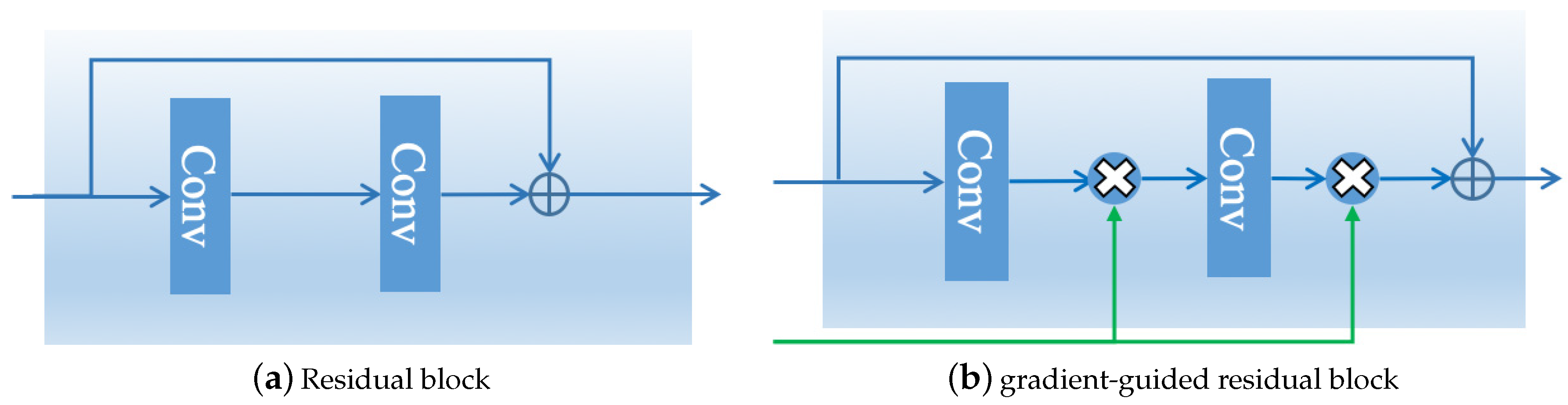
The residual network structure [32] was wildly adopted in CNN-based approaches for image super-resolution [18,21]. As illustrated in Figure 2a, the conventional residual block (Resblock) has two convolutional layers and a shortcut connection, and the result of Resblock is the addition of the input and output.
2.2. High-Frequency Details Recovery
Most CNN-based models adopt MSE as the loss function. Because MSE treats every pixel equally, it tends to produce over-smoothed results. Thus, the key objective of image SR is to recover the missing high-frequency details.
To address the over-smoothing issue, the gradient prior is widely applied in reconstruction- [4,27,30] and CNN-based MRI SR methods [33,34,35]. Image gradient provides the exact positions and magnitudes of high-frequency image parts, which are important for improving the accuracy of super-resolution performance. Two approaches are commonly used to embed the image gradient prior into CNNs:
- The image gradient is employed as a regularization item in the loss function. In a correctly restored image, the edges and texture (related to the image gradients) should be accurate. The regularization term, which is induced by additional sources of information, helps recover high-frequency details. , where is defined asin which denotes the gradient detector, and is the gradient magnitude of image x.
- The alternative approach to incorporating image gradient in the SR process is to concatenate the gradient maps with the input LR image y as a joint input of the network. Thus, the mapping function is
the above approaches implicitly assume that the input or loss function is where the gradient information should be incorporated. However, the positions of high-frequency details are not explicitly explored in the process of image reconstruction. In traditional CNN-based SR, the intermediate layers just attempt to restore the image blindly.
To encourage the network to focus on the image high-frequency details, we design a gradient-guided Resblock, which is illustrated in Figure 2b. The gradient-guided Resblock is based on Resblock, while the result of the intermediate layer is modulated using gradient information.
3. Proposed Methods
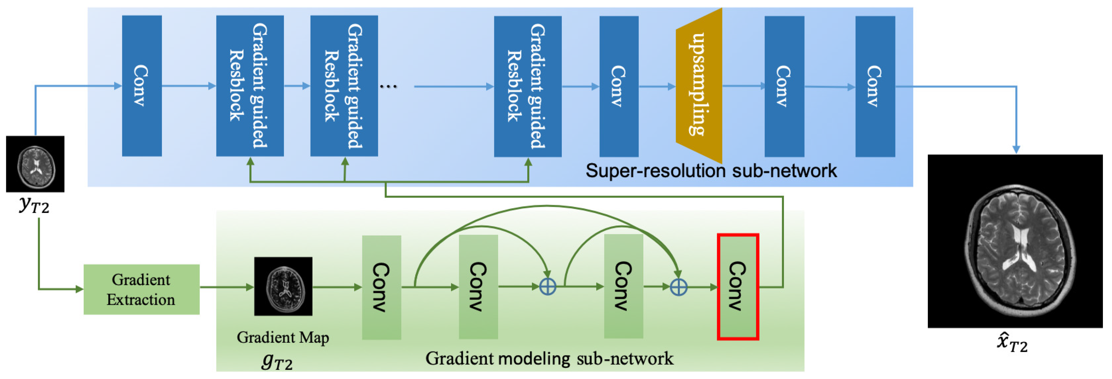
We develop a gradient-guided residual network (DGGRN) that is based on two intuitions: (1) CNN-based SR methods [12,13] have achieved significant performance advances in MRI super-resolution; and (2) gradient features of the LR image facilitate the recovery of high-frequency details in an HR image [4,28,30,34,36]. Figure 3 illustrates the main architecture of DGGRN.
DGGRN consists of two subnets. One is for gradient information modeling and the other is for super-resolution. The input of DGGRN is a LR T2w image, which is denoted as , and the output is a high-resolution image, which is denoted as .
3.1. Gradient Modeling (GM) Subnet
From the gradient magnitude map of LR T2w image , the GM subnet aims at selectively determining the locations high-frequency image details and facilitating the discrimination between smooth areas and non-smooth areas that are full of fine textures by the SR subnet. To fully exploit the gradient information for image super-resolution, the GM subnet is designed as a shallow densely connected convolutional network, so that it can be optimized end-to-end with the SR subnet.
As shown in Figure 3, the gradient detector calculates the gradient map of LR T2w image in the y- and x-directions to obtain its magnitude, and then the gradient map is normalized to before being fed into the gradient modeling subnet. Specifically, we choose Sobel detector as the gradient detector.
After normalization, is fed into the GM subnet to produce gradient guidance, which is a set of feature maps :
where is the learned mapping function with parameters . As expected, the GM subnet acts similar to a feature selector that can identify and locate high-frequency image details. We use the sigmoid function as the final convolutional layer’s activation function (shown in Figure 3 with a red box). Thus, the output of the GM subnet is a set of feature maps ranges , which provides helpful information regarding the image areas to which the information of pixels belongs. This output will be broadcast to the SR subnet to guide the SR process.
3.2. Super-Resolution Subnet
The SR subnet reconstructs the HR image conditioned on the output of GM subnet . The input of the SR subnet includes two parts, the LR T2w image and the output of GM subnet .
3.2.1. Gradient-Guided Resblock
The SR subnet consists of several gradient-guided residual blocks. We propose an effective block, namely, gradient-guided Resblock, that modulates the convolutional results according to . As illustrated in Figure 2a, compared with Resblock, the convolutional result of gradient-guided Resblock is modulated by the output of the gradient modeling.
Suppose Z is the output of the convolutional operation. The result of gradient-guided Resblock is the dot production of Z and the gradient condition :
where ⊗ denotes the element-wise multiplication. By this approach, the learned parameters of the GM subnet influence the outputs by multiplying them spatially with each intermediate feature maps in an SR subnet.
3.2.2. Reconstruction Block
In our network, we upscale features by using the sub-pixel convolutional layer [19]. The upscaling operation is performed in the latter part of the network, so that the most computations are performed in the LR space. This can reduce the number of computations while preserving the model capacity [19]. We reconstruct the final HR image :
where is the learned mapping with parameters of the SR subnet.
4. Experiments and Results
4.1. Datasets
We performed experiments on three public databases.
BrainWeb dataset [37] (http://www.bic.mni.mcgill.ca/BrainWeb/) is a publicly available MRI dataset that includes normal and multiple sclerosis simulated images. It contains a set of realistic MRI data volumes produced by an MRI simulator. The voxel dimensions of the synthetic brain MRI is mm and the data size is .
NAMIC dataset (http://hdl. handle.net/1926/1687) consists of real MRI data that were acquired using a 3T GE at BWH Hospital in Boston, MA. The voxel dimensions are mm and the data size is .
IXI dataset (https://brain-development.org/ixi-dataset/) consists of real MRI data collected from three hospitals in London. We evaluated on the MRI images from Guys hospital. The voxel dimensions are mm and the data size is .
All 3D MRI data were split into 2D image sequences along the transverse, sagittal, and coronal planes. The obtained 2D data were all normalized to .
4.2. Implementation Details
Our experiments were divided into two groups. In one group, experiments were conducted on BrainWeb and NAMIC, where we built our training set and testing set as in [13] for fair comparison. In the other group, the experiments were evaluated on the IXI dataset, where we built the training and testing sets, and then trained DGGRN from the scratch.
Training set: LR images were generated according to the following steps:
- The original image x were convolved by Gaussian kernel with standard deviation of 1.
- The results of convolution were down-sampled with factors of and 4, respectively.
The same degradation was applied in [9,13]. It aims to simulate the generation of a LR MRI image in the spatial domain.
For BrainWeb and NAMIC, we built the training sets with the same data as in [13]. For IXI dataset, 300 2D T2w images from 10 people were used for network training. By flipping and rotation, 16 augmented images were generated from each training image for data augmentation. In addition to these affine augmentations, we extended the training dataset via elastic deformation [38].
Test set: For testing, we randomly selected samples from persons excluding the training data. Specifically, we selected 56 samples from persons in IXI. The test sets of BrainWeb and NAMIC were produced as in [13].
Network structure: The SR subnet is composed of eight gradient-guided Resblocks. Each block consists of two convolutional layers. The gradient modeling subnet consists of four convolutional layers with dense connections. Following CNN-based SR studies [18,21], we set the convolutional filter 64 to . We used the method of Xavier to initialize the weights, and the biases were initialized to zero.
Training details: Our network was implemented based on Tensorflow [39]. To minimize the overhead and to fully utilize the GPU memory, the batch size was set to 64 and the training stopped after 65 epochs when no improvement was observed. The LR T2w patches and their gradient magnitude maps were fed into network as the inputs. According to the report of Pham et al. [11], the Adam method [40] provides fast convergence and better reconstruction results than SGD. Thus, we trained the network with the Adam optimization with and . The initial learning rate was which was decreased by 10% every 20 epochs.
Hardware: All experiments were conduct on a PC with a 2.1 GHz Intel Xeon E5-2620 CPU and an NVIDIA Titan X GPU (12G Memory). All compared approaches were run on the same machine.
4.3. Comparison with State-of-the-Art Methods
The proposed approach was compared with three conventional methods: bicubic interpolation low-rank and total-variation regularizations [9] and non-local up-sampling [2]. We compared our results with the CNN-based MRI SR method: single contrast super-resolution CNN (SCSR) [13] and residual-learning network (ReCNN) [11]. The SCSR was proposed for multi-contrast MRI super-resolution, and we extracted the output of its single contrast subnet for comparison. Another compared method is the most recent CNN-based method, namely ReCNN [11], which is designed for 3D MRI super-resolution. To compare our method with ReCNN, we performed the experiments according to the baseline network of [11] and trained the corresponding 2D CNN from the scratch.
To evaluate the performance of DGGRN, we trained a residual network (ResNet) with the same training data and eight Resblocks from scratch. Experiments were performed on BrainWeb and NAMIC. PSNR and structural similarity (SSIM) were used as quantitative measures. Higher PSNR values indicate the reconstructed version is more faithful to the ground-truth image, while higher SSIM values indicate that more accurate image structures are preserved. MATLAB functions were used for the evaluation.
The quantitative results of different methods are reported in Table 1. Compared with SCSR, our method yields PSNR values that are higher by approximately 1.6 dB on BrainWeb, 0.6 dB on NAMIC and 0.4 dB on IXI. DGGRN performs more competitively on the BrainWeb dataset. Our method outperforms ReCNN, which is a CNN with residual learning, for all three test sets. SSIM value corresponds to the perceptual quality of the structural similarity. The SSIM values of DGGRN are higher than other methods on real data of NAMIC and IXI. Thus, it is not trivial to embed image gradients into the CNN models.
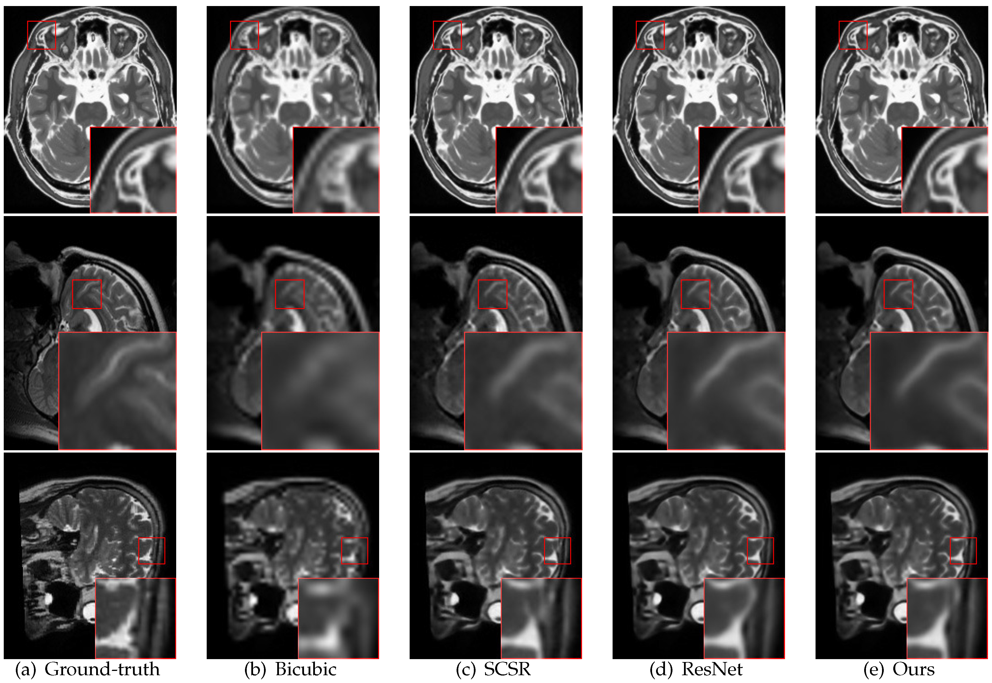
Figure 4 presents the reconstructed images of DGGRN and other methods with an upscaling factor of 4 on the three test sets. The bicubic method tends to produce blurry images with unexpected artifacts. SCSR and ResNet present more visually appealing results than bicubic method; however, they lose subtle details in some local regions. DGGRN restores more accurate image high-frequency details of edges and textures areas and recovers more informative structural details than the above methods.
5. Discussion
5.1. Benefits of Gradient-Guided Resblock
In the proposed network, the super-resolution subnet and the gradient modeling subnet are trained jointly. In Figure 5, we present some feature maps of the last convolutional layer in the gradient modeling subnet. The feature maps contain sufficient diversity for representing the high-frequency details in T2w MRI, which supports the validity of the gradient-guided strategy. Facilitated by these feature maps, the edge and texture areas can be reconstructed explicitly. In DGGRN, the SR subnet consists of eight gradient-guided Resblocks. The ResNet and the proposed network share the same initial parameters and hyperparameters, such as the learning rate and the number of epochs. Table 1 summarizes experimental results on BrainWeb and NAMIC of ResNet(the third column to last) and DGGRN (the last column). Compared with ResNet, in terms of PSNR, our network with gradient-guided realizes average improvements of 1.0 dB on BrainWeb, 0.4 dB on NAMIC and 0.3 dB on IXI.
In Figure 4, three examples of real images with an upscaling factor of 4 are presented. Facilitated by the gradient modeling subnet, the proposed method outperforms ResNet in recovering sharp edges and tiny textures.
5.2. Performance and Training Epochs
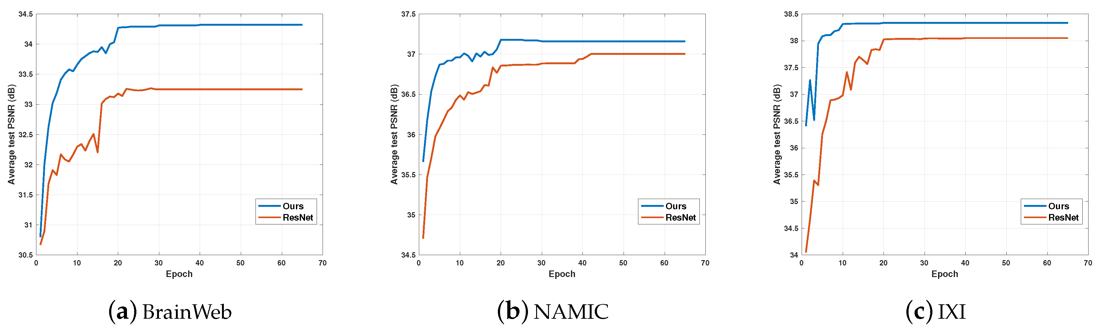
We investigated the performance and epochs of DGGRN vs. ResNet. In our work, parameters of DGGRN and ResNet were estimated by minimizing the loss function using Adam optimization. Figure 6 depicts convergence curve of DGGRN vs. ResNet with upscaling fact 2 on three test sets. It demonstrates that DGGRN converges to a plateau in 20 epochs, which represents the most appealing results. It is worth noting that DGGRN achieves higher PSNR than ResNet on all three test sets during all 65 epochs. In addition, these phenomena indicate that DGGRN converges rapidly with Adam optimization in view of both performance and convergence speed.
5.3. Parameters and Performance
Filter size: Small filter sizes such as are a popular choice in current CNN-based image super-resolution. Due to limited computational resources, CNN-based SR prefers a deeper network with small filter size rather than a wider network with large size [18,21]. Following the above studies, we set the filter size to .
Network size: One of the issues for training the deeper network is overfitting. We investigated the performance and network size based on the baseline of DGGRN (the SR subnet with eight gradient-guided Resblocks). The number of blocks was increased from 2 to 12 to evaluate the performance vs. the number of gradient-guided Resblocks. Table 2 demonstrates the PSNRs of ResNet and the proposed network with various network sizes. For DGGRN, the PSNR values are improved progressively as the number of gradient-guided Resblocks rises from 2 to 12. On the other hand, a sharp descent is observed when we try to stack more Resblocks in ResNet; the same observation was reported by Zeng et al. [13]. This might be because the gradient modeling subnet performs similar to a selector, which drops out selected inputs of the next layer to prevent overfitting.
The number of filters: The SR performance can benefit from a reasonable number of filters within networks. Thus, an appropriate number of filters K of each convolutional layer must be selected. We trained DGGRN with different K to find the appropriate value of K. It took 33, 45 and 70 s for training one epoch when , 64 and 128, respectively. Table 3 presents how the number of filters affects the performance. DGGRN denotes DGGRN with K filters. When K increases from 32 to 64, the average PSNRs of the three datasets improve about 0.56 (dB). Compared with DGGRN, DGGRN achieves little improvement (0.06 dB) in PSNR. However, both the number of parameters and training time are double those in DGGRN with 64 filters. Thus, we set as a trade-off between reconstructed image quality and the computational complexity.
6. Conclusions
A deep gradient-guided residual network is proposed in this paper for MRI super-resolution. The gradient subnetwork operates as a feature selector that enhances high-frequency features once the positions of the high-frequency details have been located. By broadcasting useful spatial information in high-frequency regions to the SR subnet, high-frequency MRI image details can be recovered explicitly. Thus, our method avoids reconstructing high-resolution images blindly. The joint recovery by the gradient modeling and super-resolution subnets leads to more accurate detail recovery. Experiments on synthetic and real brain MRI data have demonstrated that DGGRN reconstruct HR images with more faithful high-frequency details than other methods. We will explore applications of the gradient information in 3D brain MRI reconstruction in future work. Moreover, the gradient prior can be generalized to other image priors. In the future, brain image segmentation and textures and other features that describe the image can be further explored.
Author Contributions
X.D. contributed the idea and wrote the original draft; and Y.H. performed the experiments, reviewed and edited the paper.
Funding
This work was supported by the National Natural Science Foundation of China (No. 61806173), Natural Science Foundation of Fujian Province of China (No. 2019J01855 and No. 2019J01854), the Scientific Research Foundation of Xiamen for the Returned Overseas Chinese Scholars (XRS[2018] No.310).
Acknowledgments
The authors sincerely thank Kun Zeng for providing the test data and pre-process codes.
Conflicts of Interest
The authors declare no conflict of interest.
References
- Greenspan, H. Super-resolution in medical imaging. Comput. J. 2008, 52, 43–63. [Google Scholar] [CrossRef]
- Manjón, J.V.; Coupé, P.; Buades, A.; Fonov, V.; Collins, D.L.; Robles, M. Non-local MRI upsampling. Med. Image Anal. 2010, 14, 784–792. [Google Scholar] [CrossRef] [PubMed]
- Rueda, A.; Malpica, N.; Romero, E. Single-image super-resolution of brain MR images using overcomplete dictionaries. Med. Image Anal. 2013, 17, 113–132. [Google Scholar] [CrossRef] [PubMed]
- Yu, S.; Zhang, R.; Wu, S.; Hu, J.; Xie, Y. An edge-directed interpolation method for fetal spine MR images. Biomed. Eng. Online 2013, 12, 102. [Google Scholar] [CrossRef]
- Wang, Y.H.; Qiao, J.; Li, J.B.; Fu, P.; Chu, S.C.; Roddick, J.F. Sparse representation-based MRI super-resolution reconstruction. Measurement 2014, 47, 946–953. [Google Scholar] [CrossRef]
- Jafari-Khouzani, K. MRI upsampling using feature-based nonlocal means approach. IEEE Trans. Med. Imaging 2014, 33, 1969–1985. [Google Scholar] [CrossRef]
- Lu, X.; Huang, Z.; Yuan, Y. MR image super-resolution via manifold regularized sparse learning. Neurocomputing 2015, 162, 96–104. [Google Scholar] [CrossRef]
- Zhang, D.; He, J.; Zhao, Y.; Du, M. MR image super-resolution reconstruction using sparse representation, nonlocal similarity and sparse derivative prior. Comput. Biol. Med. 2015, 58, 130–145. [Google Scholar] [CrossRef]
- Shi, F.; Cheng, J.; Wang, L.; Yap, P.T.; Shen, D. LRTV: MR image super-resolution with low-rank and total variation regularizations. IEEE Trans. Med. Imaging 2015, 34, 2459–2466. [Google Scholar] [CrossRef]
- Tourbier, S.; Bresson, X.; Hagmann, P.; Thiran, J.P.; Meuli, R.; Cuadra, M.B. An efficient total variation algorithm for super-resolution in fetal brain MRI with adaptive regularization. NeuroImage 2015, 118, 584–597. [Google Scholar] [CrossRef]
- Pham, C.H.; Tor-Díez, C.; Meunier, H.; Bednarek, N.; Fablet, R.; Passat, N.; Rousseau, F. Multiscale brain MRI super-resolution using deep 3D convolutional networks. Comput. Med. Imaging Graph. 2019, 77, 101647. [Google Scholar] [CrossRef] [PubMed]
- Oktay, O.; Bai, W.; Lee, M.; Guerrero, R.; Kamnitsas, K.; Caballero, J.; de Marvao, A.; Cook, S.; O’Regan, D.; Rueckert, D. Multi-input cardiac image super-resolution using convolutional neural networks. In Proceedings of the International Conference on Medical Image Computing and Computer-Assisted Intervention, Athens, Greece, 17–21 October 2016; Springer: Cham, Switzerland, 2016; pp. 246–254. [Google Scholar]
- Zeng, K.; Zheng, H.; Cai, C.; Yang, Y.; Zhang, K.; Chen, Z. Simultaneous single- and multi-contrast super-resolution for brain MRI images based on a convolutional neural network. Comput. Biol. Med. 2018, 99, 133–141. [Google Scholar] [CrossRef] [PubMed]
- Alom, M.Z.; Taha, T.M.; Yakopcic, C.; Westberg, S.; Sidike, P.; Nasrin, M.S.; Hasan, M.; Van Essen, B.C.; Awwal, A.A.; Asari, V.K. A state-of-the-art survey on deep learning theory and architectures. Electronics 2019, 8, 292. [Google Scholar] [CrossRef]
- Cascio, D.; Taormina, V.; Raso, G. Deep CNN for IIF Images Classification in Autoimmune Diagnostics. Appl. Sci. 2019, 9, 1618. [Google Scholar] [CrossRef]
- Cascio, D.; Taormina, V.; Raso, G. Deep Convolutional Neural Network for HEp-2 Fluorescence Intensity Classification. Appl. Sci. 2019, 9, 408. [Google Scholar] [CrossRef]
- Dong, C.; Loy, C.C.; He, K.; Tang, X. Image super-resolution using deep convolutional networks. IEEE Trans. Pattern Anal. Mach. Intell. 2016, 38, 295–307. [Google Scholar] [CrossRef]
- Kim, J.; Kwon Lee, J.; Mu Lee, K. Accurate image super-resolution using very deep convolutional networks. In Proceedings of the IEEE Conference on Computer Vision and Pattern Recognition, Las Vegas, NV, USA, 26 June–1 July 2016; pp. 1646–1654. [Google Scholar]
- Shi, W.; Caballero, J.; Huszár, F.; Totz, J.; Aitken, A.P.; Bishop, R.; Rueckert, D.; Wang, Z. Real-time single image and video super-resolution using an efficient sub-pixel convolutional neural network. In Proceedings of the IEEE Conference on Computer Vision and Pattern Recognition, Las Vegas, NV, USA, 26 June–1 July 2016; pp. 1874–1883. [Google Scholar]
- Lim, B.; Son, S.; Kim, H.; Nah, S.; Mu Lee, K. Enhanced deep residual networks for single image super-resolution. In Proceedings of the IEEE Conference on Computer Vision and Pattern Recognition Workshops, Honolulu, HI, USA, 21–26 July 2017; pp. 136–144. [Google Scholar]
- Timofte, R.; Gu, S.; Wu, J.; Van Gool, L. NTIRE 2018 challenge on single image super-resolution: methods and results. In Proceedings of the IEEE Conference on Computer Vision and Pattern Recognition Workshops, Salt Lake City, UT, USA, 18–22 June 2018; pp. 852–863. [Google Scholar]
- Pham, C.H.; Ducournau, A.; Fablet, R.; Rousseau, F. Brain MRI super-resolution using deep 3D convolutional networks. In Proceedings of the 2017 IEEE 14th International Symposium on Biomedical Imaging (ISBI 2017), Melbourne, Australia, 18–21 April 2017; pp. 197–200. [Google Scholar]
- Bahrami, K.; Shi, F.; Rekik, I.; Shen, D. Convolutional neural network for reconstruction of 7T-like images from 3T MRI using appearance and anatomical features. In Deep Learning and Data Labeling for Medical Applications; Springer: Cham, Switzerland, 2016; pp. 39–47. [Google Scholar]
- Wang, S.; Su, Z.; Ying, L.; Peng, X.; Zhu, S.; Liang, F.; Feng, D.; Liang, D. Accelerating magnetic resonance imaging via deep learning. In Proceedings of the 2016 IEEE 13th International Symposium on Biomedical Imaging (ISBI), Prague, Czech Republic, 13–16 April 2016; pp. 514–517. [Google Scholar]
- Schlemper, J.; Caballero, J.; Hajnal, J.V.; Price, A.; Rueckert, D. A deep cascade of convolutional neural networks for MR image reconstruction. In Proceedings of the International Conference on Information Processing in Medical Imaging, Boone, NC, USA, 25–30 June 2017; Springer: Cham, Switzerland; pp. 647–658. [Google Scholar]
- McDonagh, S.; Hou, B.; Alansary, A.; Oktay, O.; Kamnitsas, K.; Rutherford, M.; Hajnal, J.V.; Kainz, B. Context-sensitive super-resolution for fast fetal magnetic resonance imaging. In Molecular Imaging, Reconstruction and Analysis of Moving Body Organs, and Stroke Imaging and Treatment; Springer: Cham, Switzerland, 2017; pp. 116–126. [Google Scholar]
- Hu, C.; Qu, X.; Guo, D.; Bao, L.; Chen, Z. Wavelet-based edge correlation incorporated iterative reconstruction for undersampled MRI. Magn. Reson. Imaging 2011, 29, 907–915. [Google Scholar] [CrossRef]
- Mai, Z.; Rajan, J.; Verhoye, M.; Sijbers, J. Robust edge-directed interpolation of magnetic resonance images. Phys. Med. Biol. 2011, 56, 7287–7303. [Google Scholar] [CrossRef]
- Wei, Z.; Ma, K.K. Contrast-guided image interpolation. IEEE Trans. Image Process. 2013, 22, 4271–4285. [Google Scholar]
- Zheng, H.; Zeng, K.; Guo, D.; Ying, J.; Yang, Y.; Peng, X.; Huang, F.; Chen, Z.; Qu, X. Multi-Contrast Brain MRI Image Super-Resolution With Gradient-Guided Edge Enhancement. IEEE Access 2018, 6, 57856–57867. [Google Scholar] [CrossRef]
- Sun, L.; Fan, Z.; Huang, Y.; Ding, X.; Paisley, J. A Deep Information Sharing Network for Multi-contrast Compressed Sensing MRI Reconstruction. arXiv 2018, arXiv:1804.03596. [Google Scholar] [CrossRef] [PubMed]
- He, K.; Zhang, X.; Ren, S.; Sun, J. Deep residual learning for image recognition. In Proceedings of the IEEE Conference on Computer Vision and Pattern Recognition, Las Vegas, NV, USA, 26 June–1 July 2016; pp. 770–778. [Google Scholar]
- Zhou, D.; Wang, R.; Lu, J.; Zhang, Q. Depth Image Super Resolution Based on Edge-Guided Method. Appl. Sci. 2018, 8, 298. [Google Scholar] [CrossRef]
- Xie, J.; Feris, R.S.; Sun, M.T. Edge-guided single depth image super resolution. IEEE Trans. Image Process. 2016, 25, 428–438. [Google Scholar] [CrossRef] [PubMed]
- Timofte, R.; Rothe, R.; Van Gool, L. Seven Ways to Improve Example-Based Single Image Super Resolution. In Proceedings of the IEEE Conference on Computer Vision and Pattern Recognition, Las Vegas, NV, USA, 26 June–1 July 2016; pp. 1865–1873. [Google Scholar]
- Zheng, H.; Qu, X.; Bai, Z.; Liu, Y.; Guo, D.; Dong, J.; Peng, X.; Chen, Z. Multi-contrast brain magnetic resonance image super-resolution using the local weight similarity. BMC Med. Imaging 2017, 17, 6. [Google Scholar] [CrossRef] [PubMed] [Green Version]
- Cocosco, C.A.; Kollokian, V.; Kwan, R.K.; Evans, A.C. BrainWeb: Online Interface to a 3D MRI Simulated Brain Database. NeuroImage 1997, 5, 425. [Google Scholar]
- Ronneberger, O.; Fischer, P.; Brox, T. U-net: Convolutional networks for biomedical image segmentation. In Proceedings of the International Conference on Medical Image Computing and Computer-Assisted Intervention, Munich, Germany, 5–9 October 2015; Springer: Cham, Switzerland, 2015; pp. 234–241. [Google Scholar]
- Abadi, M.; Barham, P.; Chen, J.; Chen, Z.; Davis, A.; Dean, J.; Devin, M.; Ghemawat, S.; Irving, G.; Isard, M.; et al. Tensorflow: A system for large-scale machine learning. In Proceedings of the 12th {USENIX} Symposium on Operating Systems Design and Implementation ({OSDI} 16), Savannah, GA, USA, 2–4 November 2016; pp. 265–283. [Google Scholar]
- Kingma, D.P.; Ba, J. Adam: A method for stochastic optimization. arXiv 2014, arXiv:1412.6980. [Google Scholar]
Figure 1.
The results of different super-resolution methods on real data in NAMIC with an upscaling factor of 4: (a) the ground-truth; (b) the result of SCSR [13], which tends to blur the high-frequency details; (c) the result of the residual network (ResNet); and (d) the result of our method, which is guided by gradient information during image reconstruction. More realistic results are obtained via the gradient-guided methods (zoom in for better view).

Figure 2.
Illustration of the diffidence between the residual block and the proposed gradient-guided residual block: (a) a conventional residual block; and (b) the proposed gradient-guided residual block. In (b), the output of the convolutional layer is modulated by the output of the gradient subnet.

Figure 3.
Main architecture of DGGRN. DGGRN consists of two subnets. The gradient subnet exploits gradient information and produces the clues regarding high-frequency image details based on gradient map, whereas the SR subnet aims at reconstructing the high-resolution image.
Figure 3.
Main architecture of DGGRN. DGGRN consists of two subnets. The gradient subnet exploits gradient information and produces the clues regarding high-frequency image details based on gradient map, whereas the SR subnet aims at reconstructing the high-resolution image.

Figure 4.
Super-resolution results of BrainWeb, NAMIC and IXI with an upscaling factor of 4. The results of DGGRN show superior detail recovery.
Figure 4.
Super-resolution results of BrainWeb, NAMIC and IXI with an upscaling factor of 4. The results of DGGRN show superior detail recovery.

Figure 5.
Feature maps that are generated by the last convolutional layer of the gradient modeling subnet when the training is finished. The feature maps identify the locations of edges or textures. Thus, facilitated by the feature maps, the high-frequency areas can be recovered.
Figure 5.
Feature maps that are generated by the last convolutional layer of the gradient modeling subnet when the training is finished. The feature maps identify the locations of edges or textures. Thus, facilitated by the feature maps, the high-frequency areas can be recovered.

Figure 6.
Convergence curve of DGGRN and ResNet with upscaling factor 2 on BrainWeb, NAMIC and IXI test sets. DGGRN achieves higher PSNR values than ResNet for all epochs.
Figure 6.
Convergence curve of DGGRN and ResNet with upscaling factor 2 on BrainWeb, NAMIC and IXI test sets. DGGRN achieves higher PSNR values than ResNet for all epochs.


Table 1.
The performance (PSNR/SSIM) of different methods for scale factors 2×, 3× and 4× on three datasets. Bold indicates the best performance.
Table 1.
The performance (PSNR/SSIM) of different methods for scale factors 2×, 3× and 4× on three datasets. Bold indicates the best performance.
| Dataset | Upscaling Factor | Bicubic | LRTV | NMU | SCSR | ResNet | ReCNN | Ours |
|---|---|---|---|---|---|---|---|---|
| BrainWeb | 2 | 21.51 | 24.81 | 27.50 | 32.99 | 33.25 | 32.86 | 34.32 |
| 0.827 | 0.904 | 0.952 | 0.984 | 0.985 | 0.973 | 0.987 | ||
| 3 | 18.3 | 21.67 | 21.54 | 26.07 | 27.71 | 26.10 | 27.62 | |
| 0.664 | 0.820 | 0.811 | 0.922 | 0.938 | 0.925 | 0.942 | ||
| 4 | 16.37 | 19.36 | 19.33 | 21.31 | 22.11 | 21.03 | 23.11 | |
| 0.525 | 0.697 | 0.682 | 0.776 | 0.803 | 0.771 | 0.849 | ||
| NAMIC | 2 | 28.70 | 31.98 | 33.95 | 36.86 | 37.00 | 36.64 | 37.21 |
| 0.850 | 0.910 | 0.889 | 0.922 | 0.928 | 0.920 | 0.939 | ||
| 3 | 24.93 | 29.42 | 29.34 | 31.49 | 31.52 | 31.10 | 31.97 | |
| 0.721 | 0.870 | 0.772 | 0.826 | 0.821 | 0.822 | 0.864 | ||
| 4 | 22.81 | 26.54 | 26.76 | 28.33 | 28.45 | 27.97 | 29.05 | |
| 0.613 | 0.769 | 0.642 | 0.712 | 0.717 | 0.706 | 0.737 | ||
| IXI | 2 | 28.56 | - | - | 37.86 | 38.08 | 37.31 | 38.28 |
| 0.915 | - | - | 0.982 | 0.983 | 0.970 | 0.983 | ||
| 3 | 24.68 | - | - | 31.68 | 31.79 | 31.45 | 32.06 | |
| 0.853 | - | - | 0.942 | 0.944 | 0.939 | 0.946 | ||
| 4 | 22.44 | - | - | 28.15 | 28.42 | 27.97 | 28.77 | |
| 0.723 | - | - | 0.888 | 0.893 | 0.874 | 0.895 |
Table 2.
The compared PSNR values of ResNet and our method with various network sizes.
| Block Number | 2 | 4 | 6 | 8 | 10 | 12 |
|---|---|---|---|---|---|---|
| ResNet | 36.83 | 36.96 | 37.06 | 37.00 | 14.20 | 14.20 |
| Ours | 37.00 | 37.10 | 37.18 | 37.21 | 37.16 | 37.23 |
Table 3.
The PSNR values of our method with various number of filters.
| K | 32 | 64 | 128 |
|---|---|---|---|
| BrainWeb | 32.85 | 34.32 | 34.40 |
| NAMIC | 37.13 | 37.21 | 37.23 |
| IXI | 38.16 | 38.28 | 38.38 |
© 2019 by the authors. Licensee MDPI, Basel, Switzerland. This article is an open access article distributed under the terms and conditions of the Creative Commons Attribution (CC BY) license (http://creativecommons.org/licenses/by/4.0/).
Share and Cite
MDPI and ACS Style
Du, X.; He, Y. Gradient-Guided Convolutional Neural Network for MRI Image Super-Resolution. Appl. Sci. 2019, 9, 4874. https://0-doi-org.brum.beds.ac.uk/10.3390/app9224874
AMA Style
Du X, He Y. Gradient-Guided Convolutional Neural Network for MRI Image Super-Resolution. Applied Sciences. 2019; 9(22):4874. https://0-doi-org.brum.beds.ac.uk/10.3390/app9224874
Chicago/Turabian StyleDu, Xiaofeng, and Yifan He. 2019. "Gradient-Guided Convolutional Neural Network for MRI Image Super-Resolution" Applied Sciences 9, no. 22: 4874. https://0-doi-org.brum.beds.ac.uk/10.3390/app9224874
Note that from the first issue of 2016, this journal uses article numbers instead of page numbers. See further details here.