Multi-Objective Optimization of Massive MIMO 5G Wireless Networks towards Power Consumption, Uplink and Downlink Exposure

 , , ,
, , ,  ,
,  ,
,
Abstract
:Featured Application
Abstract
1. Introduction
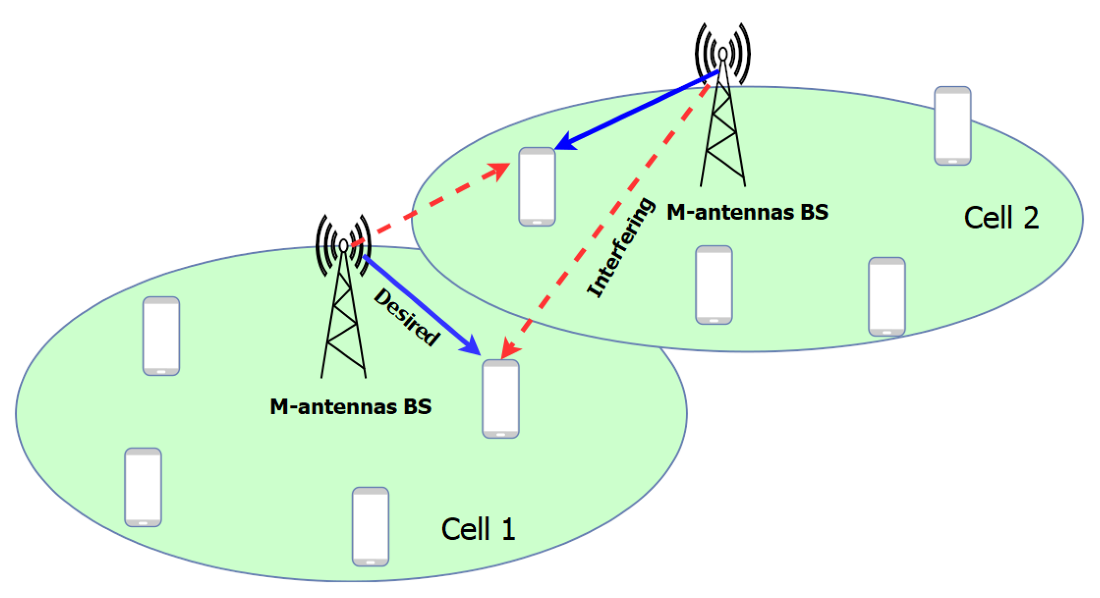
2. Massive MIMO 5G Networks
2.1. System Model
2.2. Pilot Contamination
3. Method: Massive MIMO Network Design
- A tri-objective fitness function with the downlink exposure and uplink exposure considered as two separate metrics.
- A bi-objective fitness function in which the downlink and uplink exposure are combined into a single exposure metric (the total dose).
3.1. Problem Description
3.1.1. Tri-Objective Fitness Function
- Power consumption fitness functionThe power consumption fitness function is defined as follows:where is the power consumption of the designed network in consisting of the powers consumed by the analog, the baseband and the circuit components [30]; is the power consumption of the entire network when all BSs are assumed active and transmitting at maximum power (43 ).
- Downlink exposure fitness functionThe below formula accounts for the downlink EMF exposure:where is the electric field in () within the designed network-covered area due to the downlink EMF exposure. This latter is modeled similarly to [31,32] in terms of the total EMF exposure E as the weighted average (over the area and the 40 simulations) of the median value of the electric field strengths in the area and the 95th percentile of the electric field strengths in the same area:is the maximum DL exposure in [] obtained when all BSs are assumed active and transmitting at maximum power with the maximum number of antenna elements mounted on each BS. This approach has been adopted since the favorable propagation conditions of the massive MIMO are assumed, in which the individual antenna’s propagation channels are mutually uncorrelated. and are the weighting coefficients related to and respectively and have been chosen of equal importance ().From a practical point of view, with the use of multiple antenna elements, the BS does not always transmit at maximum power since the power is split among different directions depending on the locations of the users within the area of interest [9]. So, in 5G massive MIMO BS, the realistic power level per antenna element contributing to the EMF exposure is significantly lower compared to the theoretical maximum radiated power since the duty cycles are applied (). Even for very large degrees of system utilization, the authors in [9] proved that the realistic power level can take values between 7–22%, based on the user distributions considered in both azimuth and elevation. In this analysis, since the users are uniformly distributed in azimuth, the corresponding spatial duty cycle is set to 15% [9].To evaluate the electric field created by an antenna element A of a massive MIMO 5G base station, we evaluate the DL exposure at a grid as in [32] with constant distances between two different grid points in both x-and-y axes. For each grid point i, the electric field due to A in 5G is modeled as follows [31,33]:where f is the operating frequency in ; is the path loss in ; is the theoretical maximum radiated power in ; is the TDD duty cycle in the downlink () capturing the fact that the BS does not transmit continuously and (=0.15) is the spatial duty cycle accounting for the fraction of the BS transmit power towards the direction of the user [9]. The total EMF exposure at the considered location i (grid point), due to the transmission of all N base stations in the area, each with M antenna elements, is given by the below expression:With is the EMF exposure at a location i due to a single antenna element, calculated via Equation (9).
- Uplink exposure fitness functionThe UL EMF exposure fitness function is given by the below formula:With is the uplink whole-body specific absorption rate in () due to the transmissions of the users covered by the designed network. is obtained as a weighted average of the median and the 95th percentile values over the 40 simulations and over all users:is the uplink whole-body specific absorption rate in () due to the transmission of the users at maximum transmit power (23 ). is obtained similarly to [31] in terms of weighted average as follows:The whole-body in () due to a user’s uplink traffic is obtained as per the formula below:where is the uplink duty cycle of the TDD network mode of operation. This parameter accounts for the relative transmission time with the TDD mode. Here, we assume a value of 0.25 as proposed in [9]. is the uplink reference whole-body specific absorption rate in () for 1 W of transmitted power ( = 0.0052 ()). This value has been obtained by simulations using the numerical tool (Sim4life) with 1 W of transmitting power, using a dipole at 3.7 , positioned next to the right ear. is the actual transmit power of the user’s device in (). The value of ranges from −26 to 23 . is the propagation path loss experienced by the user (in ) and is the sensitivity of the base station (in ()) for maintaining the user’s call defined as follows:With is the noise figure in () ( [34]), is the signal to noise ratio in () and is the thermal noise in () defined as follows:where is the Boltzman constant (), is the reference temperature in Kelvin () and is the bandwidth.
3.1.2. Tri-Objective Optimization Problem Formulation
3.1.3. Bi-Objective Fitness Function
- Power Consumption fitness functionHere, the fitness function that addresses the power consumption objective is similar to Equation (6).
- Dose (EMF) fitness functionThe dose fitness function accounts for the optimization of both the downlink and uplink exposure through a global metric as follows:With the total dose due to the designed network and the total dose due to the entire network when assuming all the BSs are active and working with the maximum antenna array configuration (256 antenna elements transmitting at max power and all devices active in UL with max power). The is defined by the expression below:where:
- (a)
- is the SAR (whole-body or localized) value for DL multiplied by the time spent in the configuration:With the downlink exposure duration in seconds () and the whole-body or localized induced by the BS in (). In this study, we focus on the whole-body :is the downlink reference whole-body or localized in (), obtained by means of simulations performed for a horizontal single incident plane wave with an incident power density of 1 , using numerical electromagnetic simulation software (Sim4life) and the received power density due to the base station at a location i in (), obtained as follows:With the electric field strength in [] due to a base station at a location i obtained as in Equation (10);
- (b)
3.1.4. Bi-Objective Optimization Problem Description
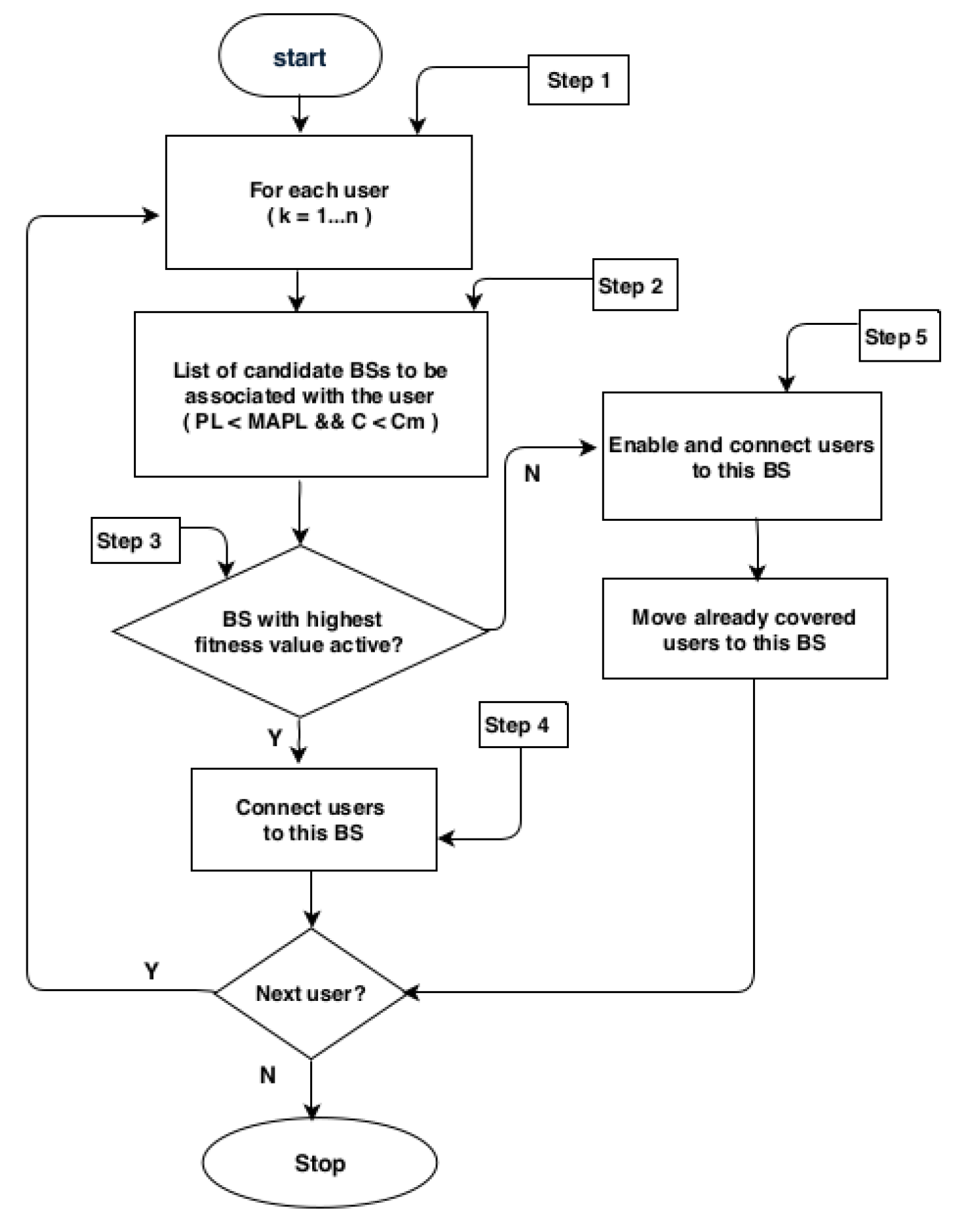
3.2. Optimization Algorithm
- For each user, the algorithm evaluates the PL between the user and all the BSs. This PL should be lower than the maximum allowable path loss (MAPL);
- The capacity C of the BS should be high enough to support the high bit rate demanded by the user u ().
- A traffic file containing the maximum number of simultaneous active users and their locations,
- The link budget parameter files (Table 2),
- The 3-dimension (3D) shapes of the environment of study,
- The power consumption file of the individual BS components.
4. Results
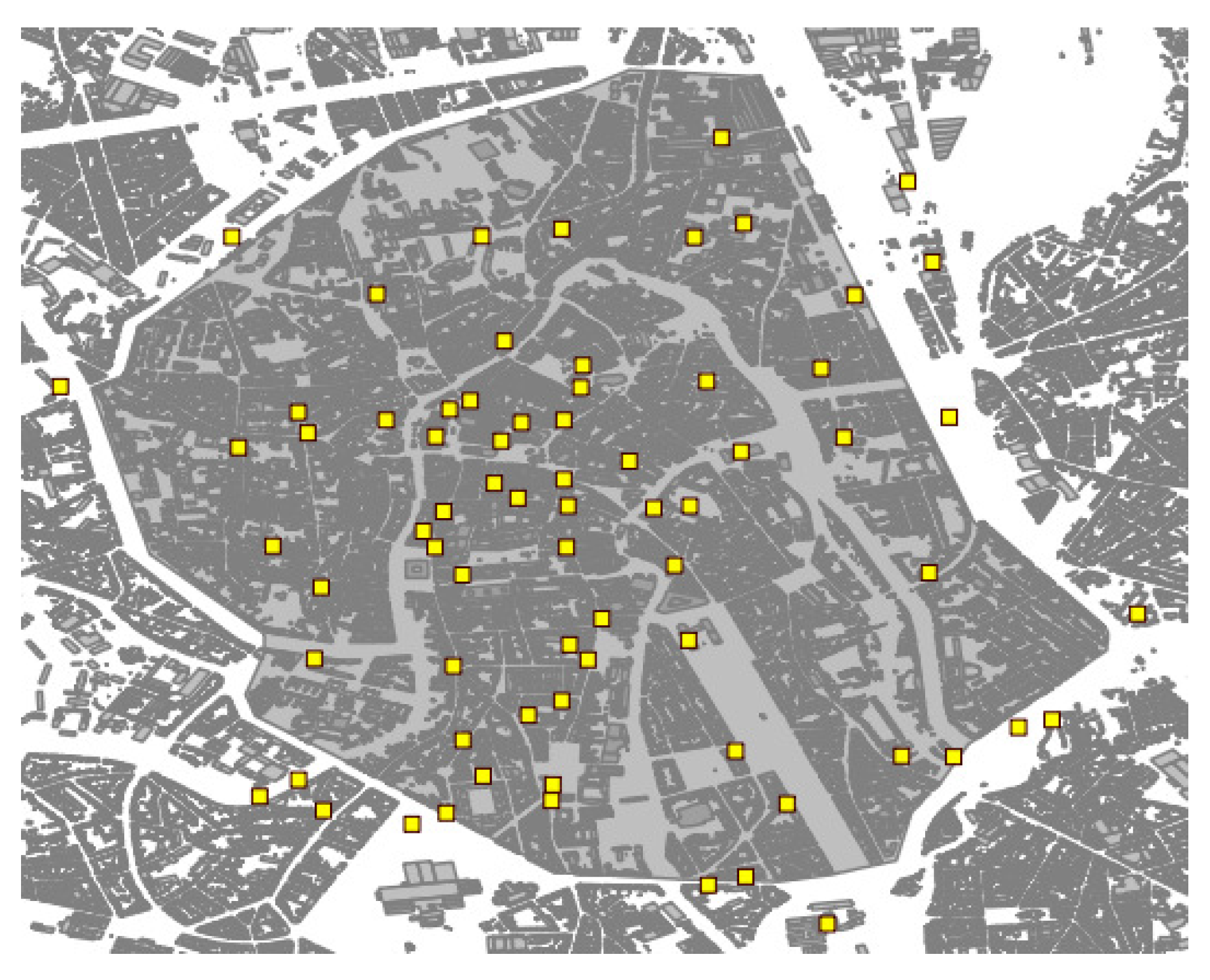
4.1. Scenarios
- Reference scenario: 4G LTE network operating at 2.6 GHz without MIMO. This is the reference network whose BS positions and power levels are optimized towards power consumption and downlink exposure. It is compared with the designed massive MIMO-LTE networks.
- Suburban information society (300 for user applications like real-time video gaming) scenarios [34]:
- –
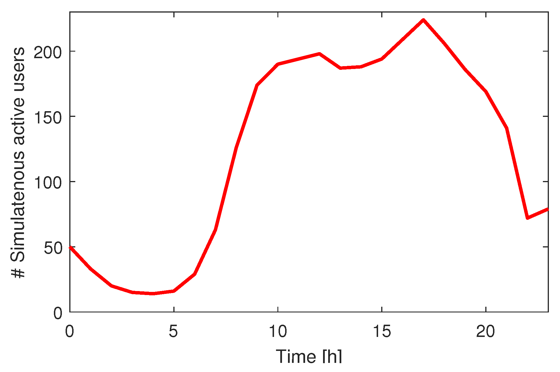
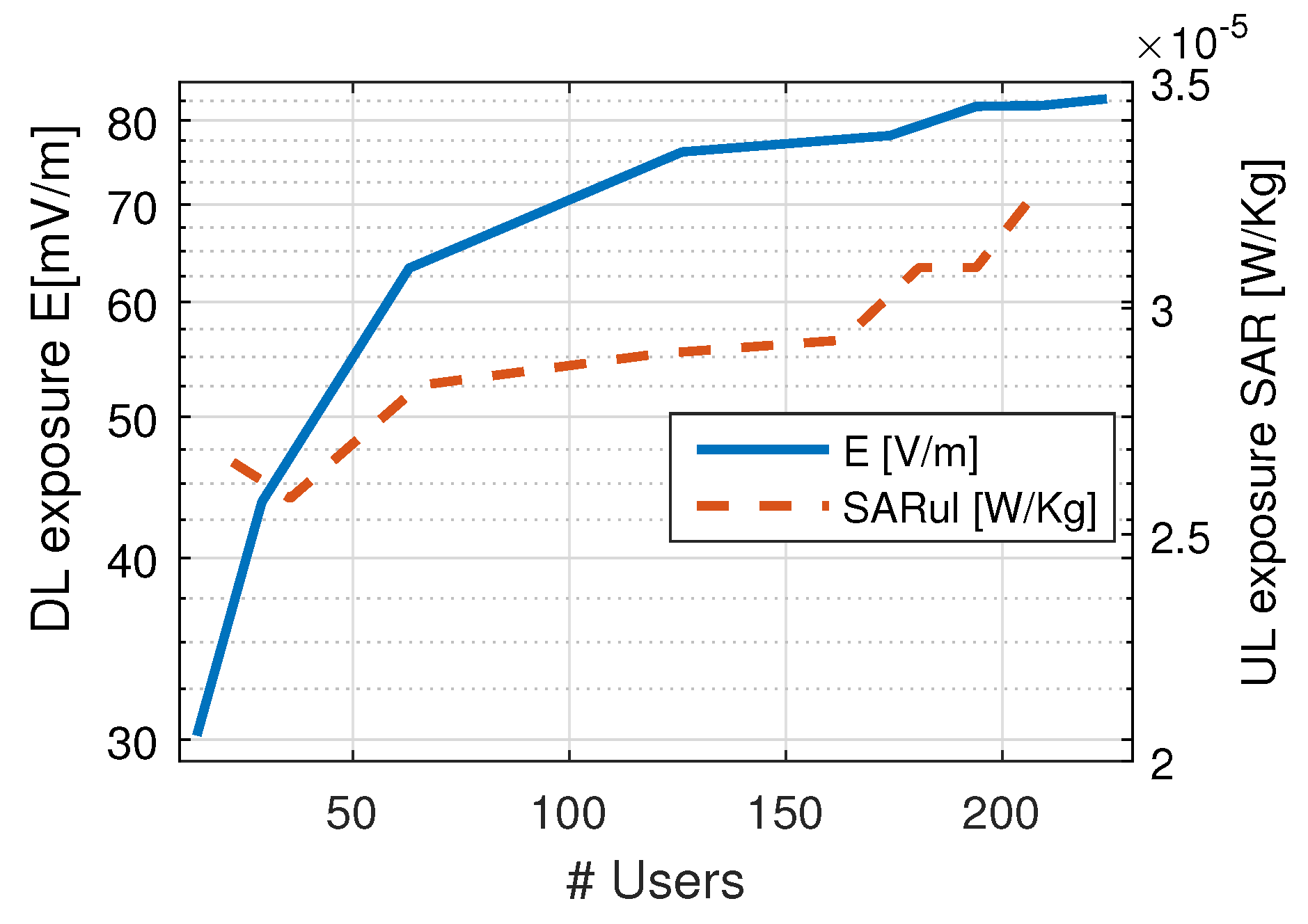
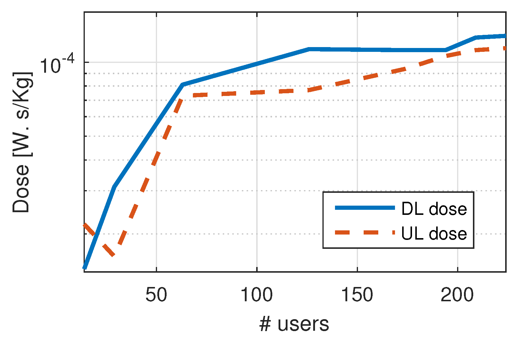
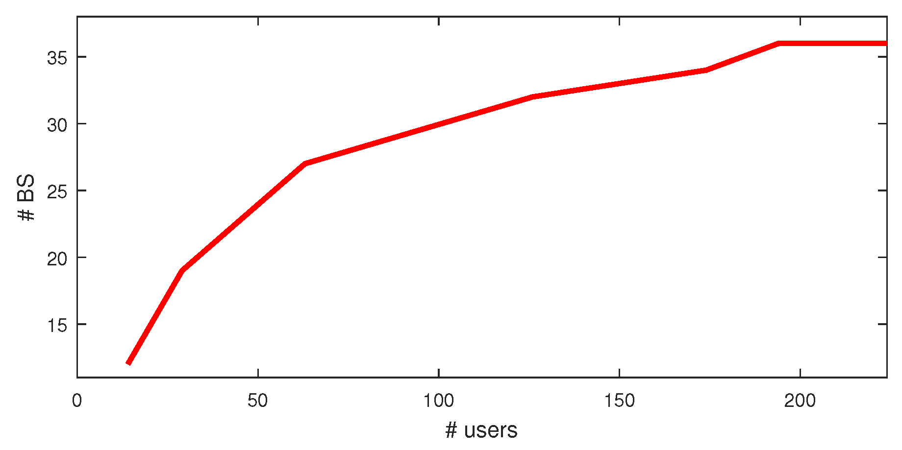
- Scenario 1: the number of users is varied, while assuming all the optimization objectives are of the same importance ( for the tri-objective optimization problem and for the bi-objective one) and the number of BS antenna elements is fixed (256 antenna elements). The number of users varies according to hourly traffic (from a Belgian mobile operator in Ghent), as presented in Figure 4.
- –
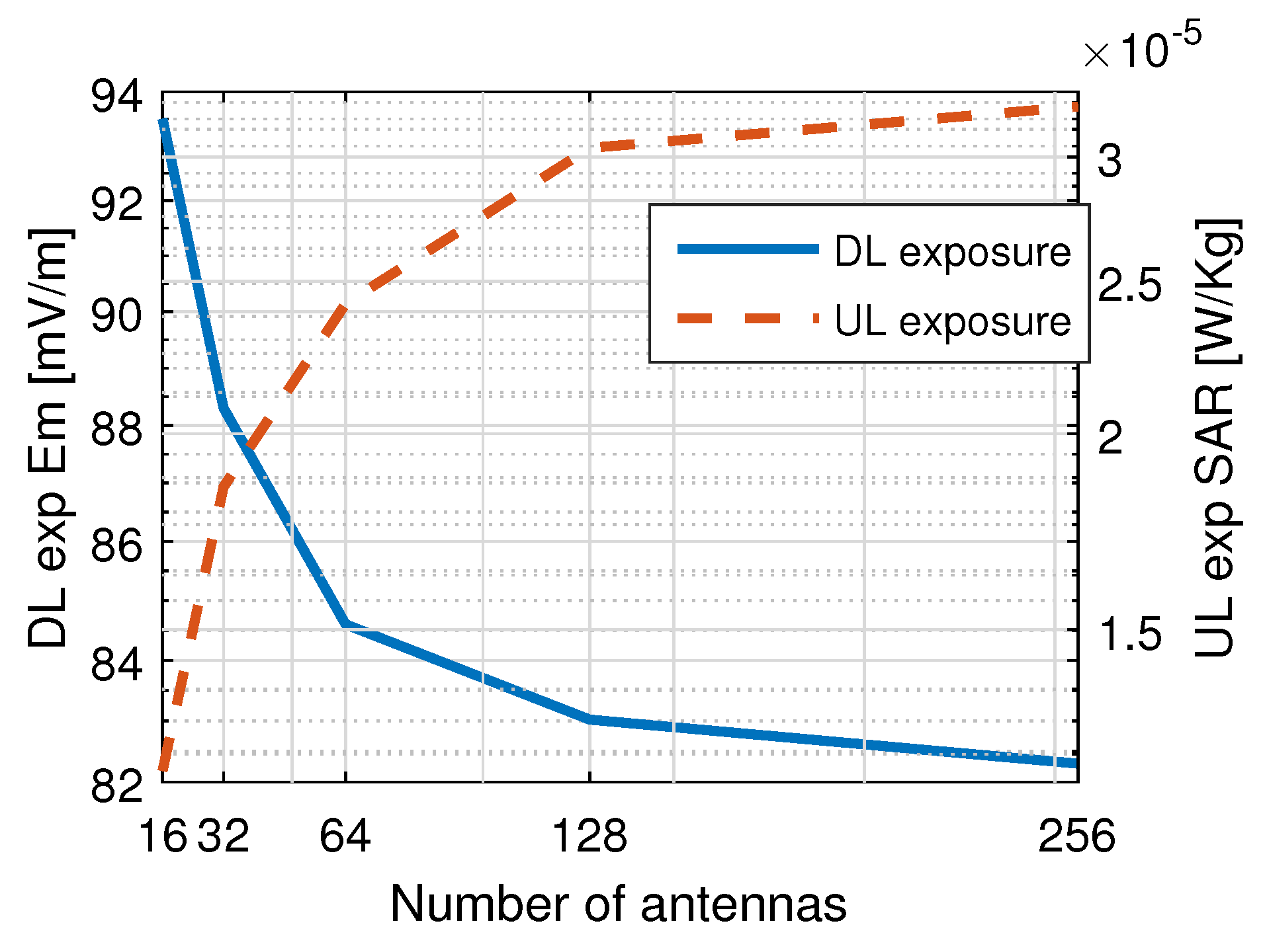
- Scenario 2: the number of BS antennas is varied while maintaining the same importance for the optimization objectives ( for the tri-objective optimization problem and for the bi-objective one). Here, the number of simultaneous active users considered for the design is fixed (224 users at busy hour, worst case scenario), while the BSs are equipped with 16, 32, 64, 128 and 256 antenna elements, respectively.
- –
- Scenario 3: The number of simultaneous active users is set to 224 users. Using some sets of combinations (), different massive MIMO networks are designed with various BS antenna elements (16, 32, 64, 128), among which only non-dominated Pareto front solutions are retained as optimal ones.
4.2. Discussion
4.2.1. Impact of the Number of Users on the EMF Exposure
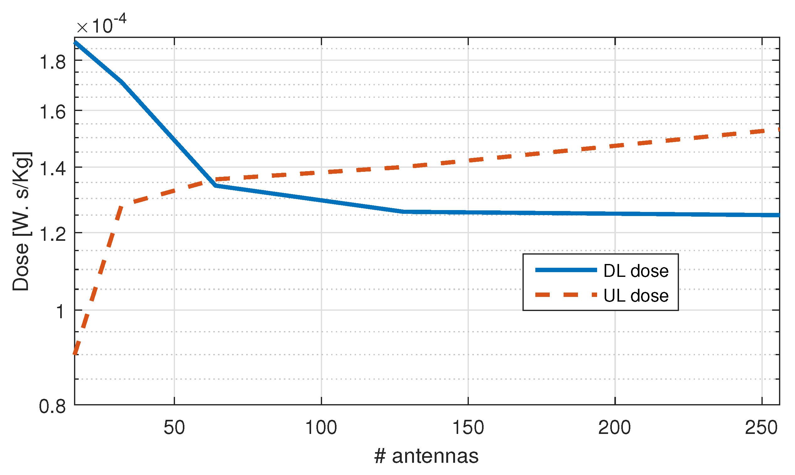
4.2.2. Impact of the Number of Antenna Elements on the EMF Exposure
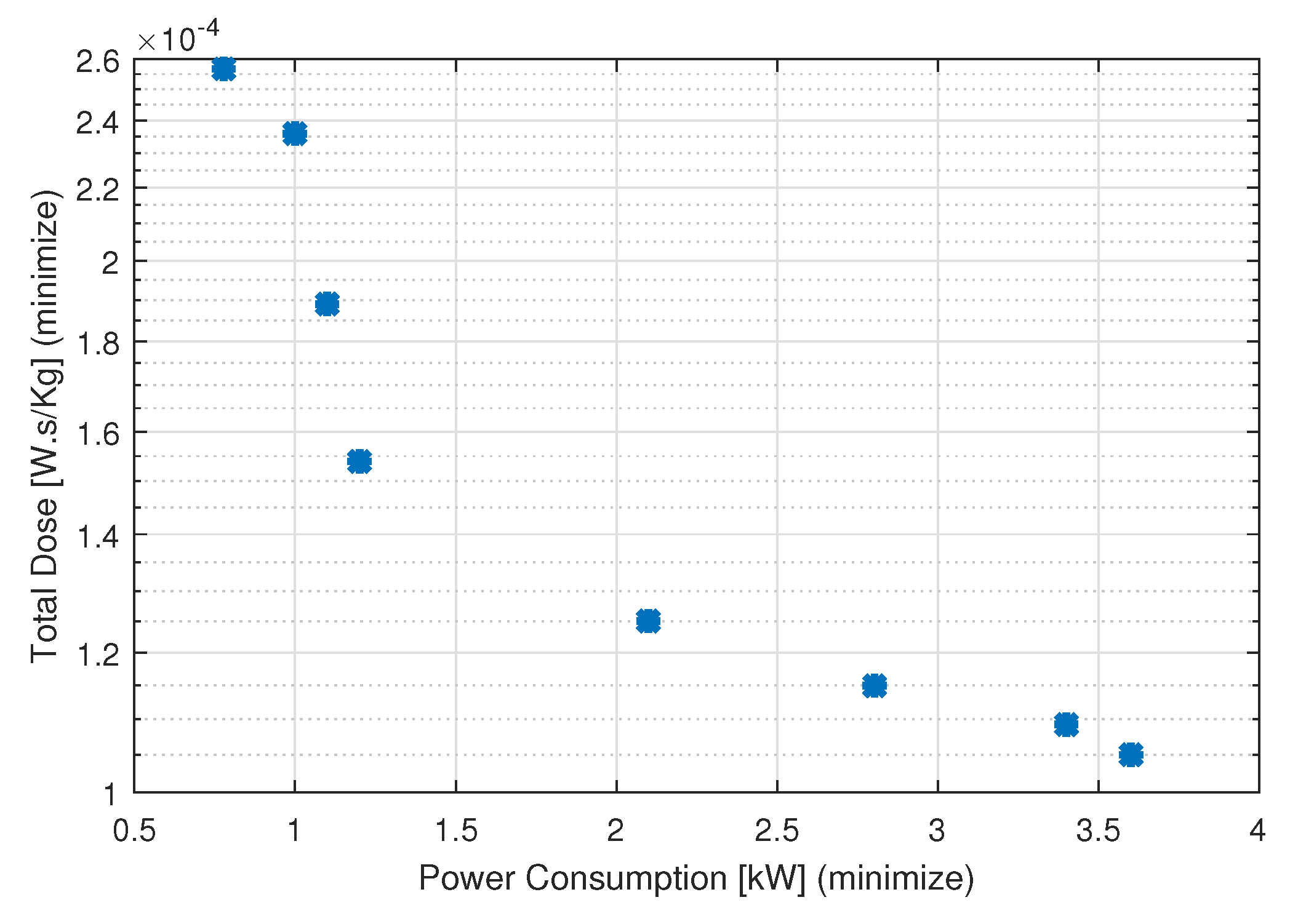
4.2.3. Pareto Front Analysis
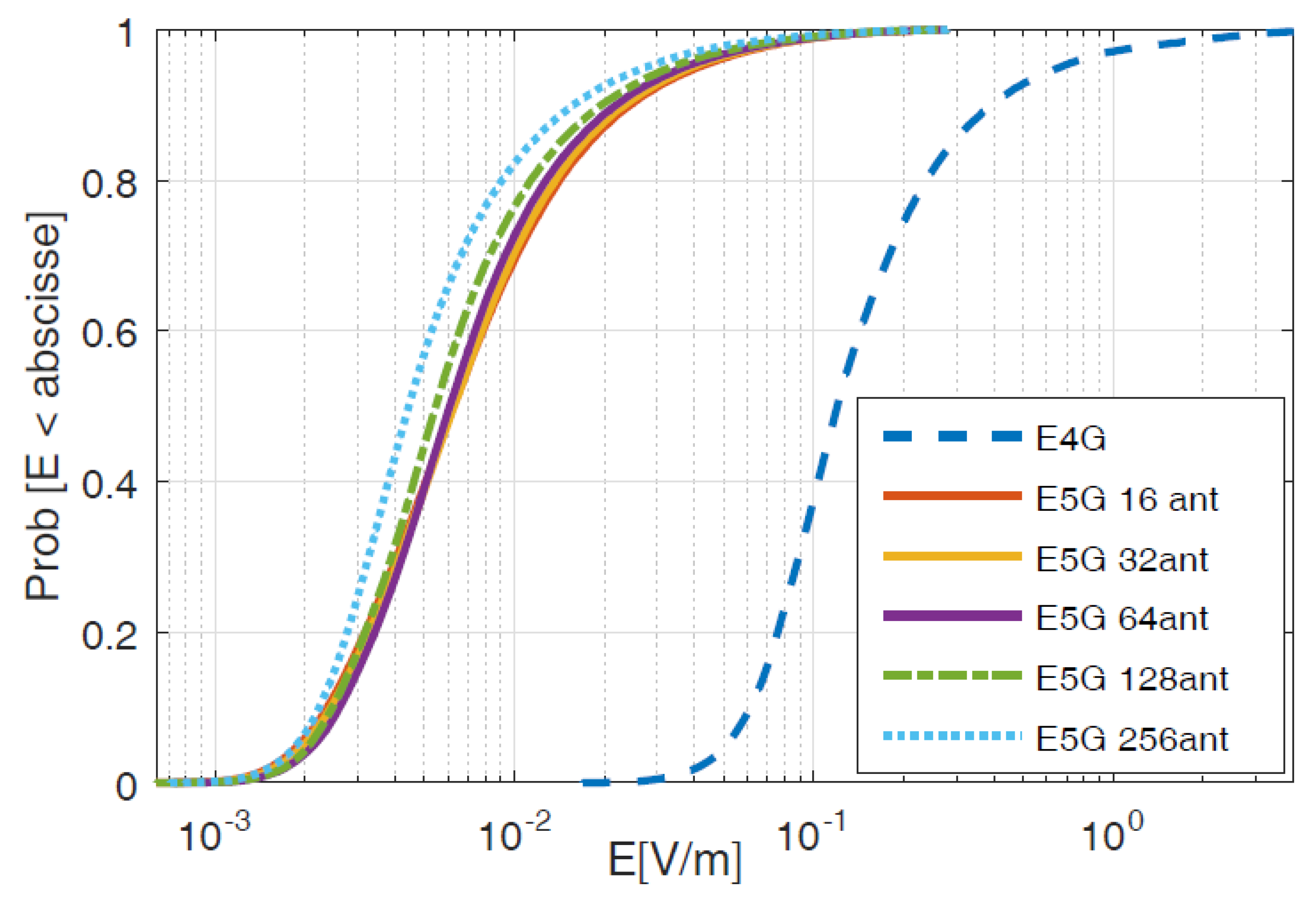
4.2.4. Comparison with 4G LTE Reference Network
5. Conclusions
Author Contributions
Funding
Acknowledgments
Conflicts of Interest
References
- Gozalvez, J. 5G Worldwide Developments [Mobile Radio]. IEEE Veh. Technol. Mag. 2017, 12, 4–11. [Google Scholar] [CrossRef]
- Larsson, E.; Edfors, O.; Tufvesson, F.; Marzetta, T. Massive MIMO for next generation wireless systems. IEEE Commun. Mag. 2014, 52, 186–195. [Google Scholar] [CrossRef]
- Björnson, E.; Larsson, E.G.; Debbah, M. Massive MIMO for Maximal Spectral Efficiency: How Many Users and Pilots Should Be Allocated? IEEE Trans. Wirel. Commun. 2016, 15, 1293–1308. [Google Scholar] [CrossRef]
- Björnson, E.; Sanguinetti, L.; Hoydis, J.; Debbah, M. Optimal design of energy-efficient multi-user MIMO systems: Is massive MIMO the answer? IEEE Trans. Wirel. Commun. 2015, 14, 3059–3075. [Google Scholar] [CrossRef]
- Chiaraviglio, L.; Cacciapuoti, A.S.; Di Martino, G.; Fiore, M.; Montesano, M.; Trucchi, D.; Melazzi, N.B. Planning 5G Networks under EMF constraints: State of the art and vision. IEEE Access 2018, 6, 51021–51037. [Google Scholar] [CrossRef]
- Thors, B.; Colombi, D.; Ying, Z.; Bolin, T.; Tornevik, C. Exposure to RF EMF from Array Antennas in 5G Mobile Communication Equipment. IEEE Access 2016, 4, 7469–7478. [Google Scholar] [CrossRef]
- Degirmenci, E.; Thors, B.; Törnevik, C. Assessment of Compliance with RF EMF Exposure Limits: Approximate Methods for Radio Base Station Products Utilizing Array Antennas with Beam-Forming Capabilities. IEEE Trans. Electromagn. Compat. 2016, 58, 1110–1117. [Google Scholar] [CrossRef]
- Baracca, P.; Weber, A.; Wild, T.; Grangeat, C. A statistical approach for RF exposure compliance boundary assessment in Massive MIMO systems. In Proceedings of the International Worshop on Smart Antennas (WSA), Bochum, Germany, 14–16 March 2018. [Google Scholar]
- Thors, B.; Furuskar, A.; Colombi, D.; Tornevik, C. Time-averaged Realistic Maximum Power Levels for the Assessment of Radio Frequency Exposure for 5G Radio Base Stations using Massive MIMO. IEEE Access 2017. [Google Scholar] [CrossRef]
- Methods for the Assessment of Electric, Magnetic and Electromagnetic Fields Associated with Human Exposure; IEC 106; IEC: Geneva, Switzerland, 2018.
- Determination of RF Field Strength and SAR in the Vicinity of the Radiocommunication Base Stations for the Purpose of Evaluating Human Exposure; IEC 62232; IEC: Geneva, Switzerland, 2011.
- Shikhantsov, S.; Thielens, A.; Vermeeren, G.; Tanghe, E.; Demeester, P.; Martens, L.; Torfs, G.; Joseph, W. Hybrid Ray-Tracing/FDTD Method for Human Exposure Evaluation of a Massive MIMO Technology in an Industrial Indoor Environment. IEEE Access 2019, 7, 21020–21031. [Google Scholar] [CrossRef]
- Dahlman, E.; Mildh, G.; Parkvall, S.; Peisa, J.; Sachs, J.; Selén, Y. 5G radio access. Ericsson Rev. (Engl. Ed.) 2014, 91, 42–47. [Google Scholar] [CrossRef]
- Plets, D.; Joseph, W.; Vanhecke, K.; Vermeeren, G.; Aerts, S.; Deruyck, M.; Martens, L. Whole-body and localized SAR and dose prediction tool for indoor wireless network deployments. In Proceedings of the 2014 11th International Symposium on Wireless Communications Systems (ISWCS) 2014, Barcelona, Spain, 26–29 August 2014; pp. 328–332. [Google Scholar] [CrossRef]
- Plets, D.; Joseph, W.; Vanhecke, K.; Vermeeren, G.; Wiart, J.; Aerts, S.; Varsier, N.; Martens, L. Joint minimization of uplink and downlink whole-body exposure dose in indoor wireless networks. Biomed Res. Int. 2015, 2015. [Google Scholar] [CrossRef] [PubMed]
- Plets, D.; Joseph, W.; Martens, L. Simulation of spatial variations of RF exposure within a macrocell. In Proceedings of the IEEE International Symposium on Antennas and Propagation and National Radio Science Meeting, San Diego, CA, USA, 9–14 July 2017. [Google Scholar]
- Varsier, N.; Plets, D.; Corre, Y.; Vermeeren, G.; Joseph, W.; Aerts, S.; Martens, L.; Wiart, J. A novel method to assess human population exposure induced by a wireless cellular network. Bioelectromagnetics 2015, 36, 451–463. [Google Scholar] [CrossRef] [PubMed]
- Marzetta, T.; Larsson, E.; Yang, H.; Quoc, H. Fundamentals of Massive MIMO; Cambridge University Press: Cambridge, UK, 2016. [Google Scholar]
- Matalatala, M.; Deruyck, M.; Tanghe, E.; Martens, L.; Joseph, W. Optimal Low-Power Design of a Multicell Multiuser Massive MIMO System at 3.7 GHz for 5G Wireless Networks. Wirel. Commun. Mob. Comput. 2018, 2018, 1–17. [Google Scholar] [CrossRef]
- Björnson, E.; Hoydis, J.; Sanguinetti, L. Massive MIMO Fundamentals and State-of-the-Art. 2018. Available online: http://www.commsys.isy.liu.se/~ebjornson/massive_MIMO_WCNC18.pdf (accessed on 12 October 2019).
- Akbar, N.; Yang, N.; Sadeghi, P.; Kennedy, R.A. Multi-Cell Multiuser Massive MIMO Networks: User Capacity Analysis and Pilot Design. IEEE Trans. Commun. 2016, 64, 5064–5077. [Google Scholar] [CrossRef]
- Chataut, R.; Akl, R. Optimal pilot reuse factor based on user environments in 5G Massive MIMO. In Proceedings of the 2018 IEEE 8th Annual Computing and Communication Workshop and Conference (CCWC), Las Vegas, NV, USA, 8–10 January 2018; pp. 845–851. [Google Scholar] [CrossRef]
- Bjornson, E.; Larsson, E.G.; Debbah, M. Optimizing multi-cell massive MIMO for spectral efficiency: How Many users should be scheduled? In Proceedings of the 2014 IEEE Global Conference on Signal and Information Processing (GlobalSIP), Atlanta, GA, USA, 3–5 December 2014; pp. 612–616. [Google Scholar] [CrossRef]
- Araujo, D.; Maksymyuk, T.; de Almeida, A.; Maciel, T.; Mota, J.; Jo, M. Massive MIMO: Survey and future research topics. IET Commun. 2016, 10, 1938–1946. [Google Scholar] [CrossRef]
- Bjornson, E.; Hoydis, J.; Sanguinetti, L. Massive MIMO Networks: Spectral, Energy, and Hardware Efficiency. Found. Trends Signal Process. 2017, 11, 154–655. [Google Scholar] [CrossRef]
- Ngo, H.; Larsson, E.; Marzetta, T. Massive mu-mimo downlink TDD systems with linear precoding and downlink pilots. In Proceedings of the 2013 51st Annual Allerton Conference on Communication, Control and Computing, Monticello, IL, USA, 2–4 October 2013; pp. 293–298. [Google Scholar]
- Jabbar, S.; Li, Y. Analysis and Evaluation of Performance Gains and Tradeoffs for Massive MIMO Systems. Appl. Sci. 2016, 6, 268. [Google Scholar] [CrossRef]
- Van Chien, T.; Björnson, E.; Larsson, E.G. Joint Power Allocation and User Association Optimization for Massive MIMO Systems. IEEE Trans. Wirel. Commun. 2016, 15, 6384–6399. [Google Scholar] [CrossRef]
- Limiting, F.O.R.; To, E.; Fields, M. Icnirp Guidelines for Limiting Exposure To Time - Varying Guidelines for Limiting Exposure To Time-Varying. Health Phys. 1998, 74, 494–522. [Google Scholar] [CrossRef]
- Desset, C.; Debaillie, B.; Louagie, F. Modeling the hardware power consumption of large scale antenna systems. In Proceedings of the 2014 IEEE Online Conf. Green Commun. OnlineGreenComm 2014, Tucson, AZ, USA, 12–14 November 2014; pp. 1–6. [Google Scholar] [CrossRef]
- Plets, D.; Wout, J.; Vanhecke, K.; Martens, L. Exposure Optimization in Indoor Wireless. Prog. Electromagn. Res. 2013, 139, 445–478. [Google Scholar] [CrossRef]
- Deruyck, M.; Tanghe, E.; Plets, D.; Martens, L.; Joseph, W. Optimizing LTE wireless access networks towards power consumption and electromagnetic exposure of human beings. Comput. Netw. 2016, 94, 29–40. [Google Scholar] [CrossRef]
- Guidance for Assessment, Evaluation and Monitoring of Human Exposure to Radio Frequency Electromagnetic Fields; ITU-T-REC-K.91; ITU: Geneva, Switzerland, 2012.
- MAMMOET. Massive MIMO for Efficient Transmission: Deliverables 1.1, Systems Scenarios and Requirements Specifications; MAMMOET: Utrecht, The Netherlands, 2014. [Google Scholar]
- Ngatchou, P.; Zarei, A.; El-Sharkawi, A. Pareto Multi Objective Optimization. In Proceedings of the 13th International Conference on Intelligent Systems Application to Power Systems, Arlington, VA, USA, 6–10 November 2005; pp. 84–91. [Google Scholar] [CrossRef]
- Matalatala, M.; Deruyck, M.; Tanghe, E.; Martens, L.; Joseph, W. Performance evaluation of 5G millimeter-wave cellular access networks using a capacity-based network deployment tool. Mob. Inf. Syst. 2017, 2017, 3406074. [Google Scholar] [CrossRef]
- Deryuck, M.; Joseph, W.; Tanghe, E.; Martens, L. Reducing the power consumption in LTE-Advanced wireless access networks by a capacity based deployment tool. Radio Sci. 2014, 49, 777–787. [Google Scholar] [CrossRef] [Green Version]
- Fixed Radio Systems; Parameters Affecting the Signal-to-Noise Ration (SNR) and the Receiver Signal Level (RSL) Threshold in Point-to-Point Receivers; ETSI TR 103 053; ETSI: Sophia Antipolis, France, 2014; pp. 1–22.


| Parameters | Symbols | Values | Units |
|---|---|---|---|
| Reference Specific | 0.0048 | ||
| Absorption Rate DL | |||
| Reference Specific | 0.0052 | ||
| Absorption Rate UL | |||
| TDD duty cycle in DL | 0.75 | [-] | |
| TDD duty cycle in UL | 0.25 | [-] | |
| Spatial duty cycle in DL | 0.15 | [-] | |
| Time duration in DL | 3600 | s | |
| Time duration in UL | 35 | s |
| Parameters | Values |
|---|---|
| Carrier frequency | 3.7 GHz 1 |
| Channel bandwidth | 20 MHz 1 |
| Transmit antenna element gain | 0 dBi |
| Transmit array antenna feed loss | 3 dB |
| Base Station Total radiated power | 43 dBm |
| Number of MS antenna elements | 1 |
| MS transmit power | 23 dBm |
| Receive antenna element gain | 0 dBi 1 |
| SNR | (7.5,15.5,17.2) dB 2 |
| Implementation loss | 3 dB |
| RX Noise figure | 7 dB |
| Other losses (Shadow, fading) | 20 dB |
| Scenarios | #BS Ant/#Users | # BS | Power (kW) | DL Em (mV/m) | UL SAR | User Cov. (%) | |
|---|---|---|---|---|---|---|---|
| (-) | (W/Kg) | (-) | |||||
| different # users | 256/14 | 12 | 1.5 | 30.2 | 0.87/0.94/0.96 | 100.0 | |
| 256/29 | 17 | 2.1 | 43.7 | 0.82/0.95/0.9 | 96.5 | ||
| 256/63 | 27 | 3.9 | 63.3 | 0.68/0.93/0.89 | 95.3 | ||
| 256/126 | 33 | 4.8 | 76.1 | 0.66/0.93/0.88 | 97.6 | ||
| 256/174 | 35 | 5.1 | 78.1 | 0.58/0.92/0.88 | 95.9 | ||
| 256/194 | 36 | 5.6 | 81.8 | 0.53/0.91/0.88 | 96.9 | ||
| 256/209 | 33 | 5.1 | 81.9 | 0.54/0.9/0.87 | 96.3 | ||
| 256/224 | 36 | 5.6 | 82.78 | 0.51/0.91/0.87 | 96.0 | ||
| different # antennas | 16/224 | 48 | 1 | 93.5 | 0.92/0.91/0.95 | 89.7 | |
| 32/224 | 48 | 1.4 | 88.3 | 0.91/0.93/0.92 | 90.4 | ||
| 64/224 | 46 | 2.3 | 84.6 | 0.81/0.88/0.9 | 93.3 | ||
| 128/224 | 42 | 3.4 | 83.0 | 0.83/0.89/0.88 | 95.9 | ||
| 256/224 | 36 | 5.6 | 82.3 | 0.99/0.84/0.98 | 96 |
| Scenarios | #BS Ant/#Users | # BS | Power (kW) | DL Dose | UL Dose | Total Dose | User Cov. (%) | |
|---|---|---|---|---|---|---|---|---|
| (-) | [-] | |||||||
| different # users | 256/14 | 10 | 1.4 | 0.87/0.98 | 100.0 | |||
| 256/29 | 19 | 2.9 | 0.82/0.97 | 100 | ||||
| 256/63 | 27 | 4.1 | 0.65/0.96 | 96.9 | ||||
| 256/126 | 32 | 4.7 | 0.58/0.98 | 96 | ||||
| 256/174 | 34 | 5.2 | 0.56/0.96 | 96.6 | ||||
| 256/194 | 34 | 5.4 | 0.52/0.97 | 94.8 | ||||
| 256/209 | 36 | 5.6 | 0.58/0.95 | 95.7 | ||||
| 256/224 | 36 | 5.6 | 0.58/0.95 | 96 | ||||
| different # antennas | 16/224 | 47 | 1 | 0.94/0.96 | 88.5 | |||
| 32/224 | 47 | 1.4 | 0.9/0.92 | 90 | ||||
| 64/224 | 45 | 2.2 | 0.82/0.9 | 93.8 | ||||
| 128/224 | 43 | 3.6 | 0.81/0.9 | 94.8 | ||||
| 256/224 | 36 | 5.6 | 0.56/0.95 | 96 | ||||
| Best compromised solution () | 64/224 | 37 | 2.1 | 0.94/0.96 | 93.5 |
© 2019 by the authors. Licensee MDPI, Basel, Switzerland. This article is an open access article distributed under the terms and conditions of the Creative Commons Attribution (CC BY) license (http://creativecommons.org/licenses/by/4.0/).
Share and Cite
Matalatala, M.; Deruyck, M.; Shikhantsov, S.; Tanghe, E.; Plets, D.; Goudos, S.; Psannis, K.E.; Martens, L.; Joseph, W. Multi-Objective Optimization of Massive MIMO 5G Wireless Networks towards Power Consumption, Uplink and Downlink Exposure. Appl. Sci. 2019, 9, 4974. https://0-doi-org.brum.beds.ac.uk/10.3390/app9224974
Matalatala M, Deruyck M, Shikhantsov S, Tanghe E, Plets D, Goudos S, Psannis KE, Martens L, Joseph W. Multi-Objective Optimization of Massive MIMO 5G Wireless Networks towards Power Consumption, Uplink and Downlink Exposure. Applied Sciences. 2019; 9(22):4974. https://0-doi-org.brum.beds.ac.uk/10.3390/app9224974
Chicago/Turabian StyleMatalatala, Michel, Margot Deruyck, Sergei Shikhantsov, Emmeric Tanghe, David Plets, Sotirios Goudos, Kostas E. Psannis, Luc Martens, and Wout Joseph. 2019. "Multi-Objective Optimization of Massive MIMO 5G Wireless Networks towards Power Consumption, Uplink and Downlink Exposure" Applied Sciences 9, no. 22: 4974. https://0-doi-org.brum.beds.ac.uk/10.3390/app9224974