Deep Multiphysics and Particle–Neuron Duality: A Computational Framework Coupling (Discrete) Multiphysics and Deep Learning


School of Chemical Engineering, University of Birmingham, Birmingham B15 2TT, UK
Appl. Sci. 2019, 9(24), 5369; https://0-doi-org.brum.beds.ac.uk/10.3390/app9245369
Submission received: 11 November 2019
/
Revised: 4 December 2019
/
Accepted: 6 December 2019
/
Published: 9 December 2019
Abstract
:Featured Application
Coupling First-Principle Modelling with Artificial Intelligence.
Abstract
There are two common ways of coupling first-principles modelling and machine learning. In one case, data are transferred from the machine-learning algorithm to the first-principles model; in the other, from the first-principles model to the machine-learning algorithm. In both cases, the coupling is in series: the two components remain distinct, and data generated by one model are subsequently fed into the other. Several modelling problems, however, require in-parallel coupling, where the first-principle model and the machine-learning algorithm work together at the same time rather than one after the other. This study introduces deep multiphysics; a computational framework that couples first-principles modelling and machine learning in parallel rather than in series. Deep multiphysics works with particle-based first-principles modelling techniques. It is shown that the mathematical algorithms behind several particle methods and artificial neural networks are similar to the point that can be unified under the notion of particle–neuron duality. This study explains in detail the particle–neuron duality and how deep multiphysics works both theoretically and in practice. A case study, the design of a microfluidic device for separating cell populations with different levels of stiffness, is discussed to achieve this aim.
1. Introduction
Today, machine learning is used in a variety of fields. However, it normally produces black-box models that are not based on the underlying physics, chemistry or biology of the system under investigation. To alleviate this issue, a variety of approaches combine first-principle modelling (FPM) with machine learning (ML). Examples are data-driven modelling and clustering. In Ibañez et al. [1], for instance, ML was used to extract constitutive relationships in solid mechanics directly from data, while in Snyder et al. [2], ML was used to learn density functionals. Other methodologies include reduce-order modelling and field-reconstruction. The idea is to use ML to learn from data generated by expensive computational models and produce a black-box model capable of imitating the output of the FPM with lower computational costs. This approach is used in turbulence [3], where the ML algorithm is trained with data generated by direct numerical simulations (DNS) and is used as an additional term in less expensive Reynolds-averaged Navier–Stokes (RANS) models. Liang et al. [4] used a similar idea in solid mechanics: stress distribution data generated by finite element analysis were fed into neural networks to train the network to quickly estimate stress distributions.
In all the examples above, the coupling between FPM and ML is in series: the two components remain distinct, and data generated by one model are subsequently fed into the other. However, as explained in [5], in-series coupling is not satisfactory for problems such as in-silico modelling of human physiology. Computer simulations of human organs, for instance, should account for the active intervention of the autonomous nervous system (ANS) that responds dynamically to environmental stimuli, ensuring the correct functioning of the body. Since it is not currently possible to model the ANS by first-principles, Alexiadis [5] used Artificial Intelligence (AI)to replicate the activity of the ANS in the case of peristalsis in the oesophagus. This approach requires a constant and localized exchange of information between the first-principles (FP) model and the ML algorithm. Biological neurons, in fact, are dispersed all over the surface of the oesophagus, and their activation is temporarily and spatially dependent on the physical interaction between the food and the oesophagus, which are calculated by the FP model and evolve continuously during the simulation. For this reason, in this case we cannot adopt in-series coupling, where the FP simulation and the ML algorithm occur separately (i.e., in series (one after the other)); we need a different approach, where the two models work together (i.e., in parallel (at the same time)). In this study, this new approach is called ‘in parallel’ as opposite to the traditional approach defined as ‘in series’; the reader should not confuse this terminology with the parallel or serial programming paradigms that can be used to numerically implement both FPM and ANNs.
Deep multiphysics is a computational framework that allows for this type of parallel coupling between FPM and ML. It is based on the so-called particle–neuron duality and has discrete multiphysics (DMP) and artificial neural networks (ANNs) as special cases. In Alexiadis 2019 [5], deep multiphysics was applied to human physiology, but since that study was based on reinforcement learning [6] rather than ANNs, the particle–neuron duality stayed in the background and was not discussed in detail. The present paper fills this gap by focusing on the framework rather than the application. A practical example (cell sorting based on the rigidity of the external membrane) is presented as a mean to facilitate the understanding of how particle duality works.
This article is divided into three parts: the first provides an introduction to discrete multiphysics, the second introduces the general framework for coupling discrete multiphysics (DMP) with artificial neural networks (ANN) and the third applies this concept to a practical application (e.g., design of microfluidic devices for the identification and separation of leukemic cells).
2. Discrete Multiphysics
Different from traditional multiphysics, discrete multiphysics is a mesh-free multiphysics technique based on ‘computational particles’ rather than on computational meshes [7,8]. It is a hybrid approach that combines different particle methods such as smoothed particle hydrodynamics (SPH), the lattice-spring model (LSM) and the discrete element method (DEM). The algorithm of particle methods, such as SPH, LSM and DEM, follows the same flowchart (Figure 1a), with the only difference being how the internal forces are calculated. In solid-liquid flows, for instance, there are three types of forces: (i) pressure and viscous forces occurring in the liquid, (ii) elastic forces occurring in the solid and (iii) contact forces occurring when two solids collide with each other. In discrete multiphysics, these forces are achieved by means of three different particle-based methods (Figure 1b): (i) SPH for the liquid, (ii) LSM for the solid and (iii) DEM for the contact forces. Boundary conditions (BC) are also represented by forces: non-compenetration, for instance, is achieved by means of repulsive forces preventing particles overlapping [8]. DMP, therefore, is a metamodel, i.e., a framework for coupling different models within multiphysics simulations. SPH, LSM and DEM are the most common models in DMP, but other choices are possible as long as they follow the flowchart of Figure 1a. Fluctuating hydrodynamics, for instance, could include Brownian dynamics (BD) to account for Brownian fluctuations in the flow.
Discrete multiphysics has proven to be more than just an alternative to traditional multiphysics. There is a variety of situations where DMP tackles problems that are very difficult, if not impossible, for traditional multiphysics. In traditional multiphysics, domains are assigned during pre-processing: the user establishes, before the simulation, which part of the domain belongs to the solid domain and which part to the fluid domain: this choice cannot change during the simulation. In DMP, the distinction between solid and fluid only depends on the type of force applied to the computational particles and, by changing the type of force, we can change the behaviour of the particles from solid to liquid and vice versa, during the simulation. In the case of solidification, for instance, when the internal energy of a particle goes below a given value, the model used to simulate that particular particle is switched from SPH to LMS. This confers an advantage to discrete multiphysics in a variety of cases (Figure 2) such as cardiovascular flows with blood agglomeration [9,10,11], phase transitions [12], capsules and cells breakup [13,14] and dissolution problems [8,15].
In addition, the particle framework of DMP has proven to be particularly effective when coupled with artificial intelligence (AI) algorithms. In [5], DMP was coupled with reinforcement learning (RL) to account for the effect of the autonomic neural system in multiphysics simulations of human physiology. As a benchmark case, the DMP + RL approach was used for a computer model of the oesophagus with the ability to learn by itself how to coordinate its contractions and propel food in the right direction. In this article, I show that, by establishing particle–neuron duality, DMP can also be effectively coupled with another type of AI algorithm: artificial neural networks.
3. From Discrete Multiphysics to Deep (Discrete) Multiphysics
This section provides a brief introduction to artificial neural networks followed by the description of the particle–neuron duality.
3.1. Artificial Neural Networks
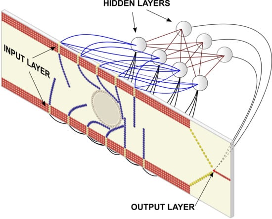
Artificial neural networks (ANN) are computer systems used to solve complex problems. The building block of an ANN is the McCulloch–Pitts neuron [16], a mathematical function vaguely inspired by the functioning of biological neurons (Figure 3a).
Several inputs xn enter the neuron; each of these inputs is multiplied by a weight wn, summed together, and fed to an activation function σ, which produces the output y. When many of these neurons are interconnected, they form an artificial neural network [17]. Typically, these networks are organized in layers: input data are introduced via an input layer, which communicates to one or more hidden layers and, finally, to an output layer (Figure 3b). The weighted output of each layer is fed as input of the next layer until the output layer calculates the final output of the network. An artificial neural network (ANN) with multiple layers between the input and output layers is called a deep neural network.
Deep neural networks are universal approximate functions, meaning that, given a large enough number of neurons in the hidden layer, they can approximate almost any function, no matter how complicated. To achieve this goal, the ANN needs to be trained. We provide the machine with real-word data (xn, y) and, by using a learning rule (e.g., backpropagation [18]), the ANN modifies its weights to correctly map xn to y.
3.2. The Particle–Neuron Duality
As mentioned above, discrete models, such SPH, LSM and DEM, work by exchanging forces among computational particles (Figure 4a). These forces change the velocity and the position of the particles and, by doing that, the model achieves a discrete representation of the mechanics.
Besides velocity and position, computational particles can have other properties. In heat transfer problems, for instance, particles require a new property called ‘temperature’. If we want this property to behave like the physical temperature, we must link it to the heat transfer equation. In this case, the particles do not exchange forces, but rather more general interactions that simulate the physical process of heat transfer from one computational particle to another (Figure 4b). This can be generalized to any conservation law: we assign a new property to the particles, and the corresponding transfer equation calculates the interactions that dynamically evolve this property with time.
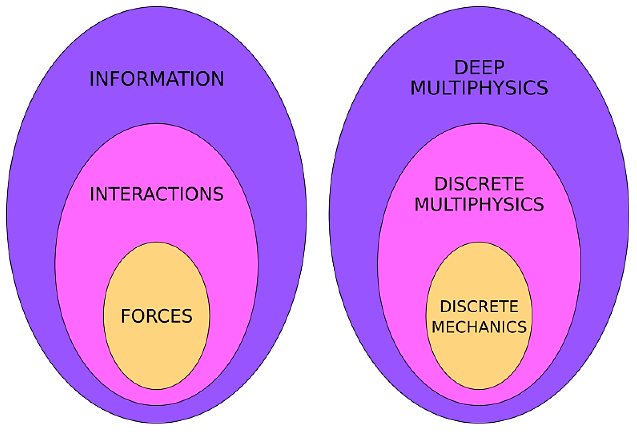
Interactions are more general than forces. If we only account for forces, we have a ‘discrete mechanics’ tool that is limited to momentum-conservation problems. If we include interactions, we have a ‘discrete multiphysics’ tool that applies to a wider variety of conservation problems. Discrete multiphysics, therefore, is a generalization of discrete mechanics (Figure 5).
The next question, at this point, would be: can we generalize this idea even further? In addition, to achieve this, what concept, more general than ‘interaction’, can we use?
Information is the most general exchange of ‘something’ we can think of. Whenever two computational particles exchange forces, interactions or any other property, they exchange information.
The exchange of information is exactly what happens in ANNs, where information is transferred from one neuron to another (Figure 4c). In the case of ANNs, this information has no direct connection with any physical property. However, ‘physical interactions’ or ‘physical forces’ can be seen as a form of information transfer and, as such, a subset of the more general concept of ‘information’ (Figure 5).
This idea constitutes the basis of the particle–neuron duality we use to establish the general framework of deep discrete Multiphysics (or simply deep multiphysics). The elemental building block of deep multiphysics is a particle–neuron hybrid: it behaves like a DMP particle when it carries out physical interactions and like a neuron when it exchanges non-physical information, and, like a neuron, it can be trained.
To illustrate and clarify this point, the rest of the article focuses on a case study where practical implementation of deep multiphysics is presented.
4. Practical Implementation: Identification and Separation of Leukemic Cells from Healthy Ones
As a practical example, I use deep multiphysics to design a microfluidic device that, potentially, can be used to separate leukemic cells from healthy ones in the peripheral circulation system.
In Section 4.1, I describe the biomedical rationale for such a device, while in Section 4.2 and Section 4.3, I explain the deep multiphysics model used for the calculations.
4.1. Leukemic Cell Detection: Biomedical Rationale
Acute myeloid leukaemia is a malignant neoplasm of the bone marrow accounting for 10% of all haematological disorders. Although in recent years new therapeutic approaches have been devised, the overall survival of patients is less than 30%. This is mostly due to the high rate of disease relapse that is observed in patients treated with standard targeted chemotherapy. After treatment, the disease is often not completely eradicated, and leukemic cells still persist although in numbers that are below detectable levels by standard means. A microfluidic device that can easily distinguish malignant from healthy cells, therefore, would be extremely useful. Most common microfluidics separation techniques, however, work with cells of different sizes, but, in the present case, this would not work since malignant and healthy cells are approximately the same size.
The proposed solution takes advantage of the fact that malignant cells are more flexible than healthy ones. A microchannel is lined with several hair-like flexible structures that, in the rest of the paper, are called cilia. When cells move along the channel, the cilia bend to allow the passage of the cells. When cilia bend, stresses are generated at their base. The idea of the microfluidic separator is to distinguish between rigid or flexible cells by looking at the stress patterns occurring during their passage. In a real device, these stresses could be measured by using a piezoelectric material at the base of the cilia. AI is used to associate specific stress patterns with the stiffness of the cell.
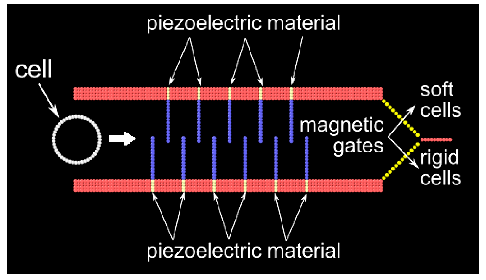
The geometry of the microfluidic device is shown in Figure 6: the length of the channel is 200 μm, and the width is 50 μm. In the channel, there are 11 flexible cilia: 6 on the upper wall and 5 on the lower wall. The distance between two contiguous cilia is 20 μm. At the right end of the channel, there are two gates, one that connects the channel with a chamber where soft cells are collected and another that connects with a chamber where rigid cells are collected. In a real device, a magnet can be used to open or close these gates. However, this study focuses on the modelling aspects, and I do not deal here with the more technical aspects of building the microchannel.
In Section 4.2, the DMP model of the device is introduced. In Section 4.3, the model is coupled with an ANN to obtain a deep multiphysics model.
4.2. The DMP Model
Figure 6 shows the (two-dimensional) domain used in the simulations. The lattice spring model (LSM), which models the mechanical properties of solid material by means of linear bonds and angular springs, is used for both the cilia and the cell. In this study, all bonds are rigid (i.e., inextensible) with fixed distance Δr = 2 μm, while the force F generated by an angular spring that connects three consecutive particles is given by the gradient of the potential
where k is the stiffness of the spring, θ0 the equilibrium angle at rest, and θ the angle after deformation. In a real microfluidic application, liquid would flow into the device and convey the cells by means of drag forces. To simplify the model, liquid is not directly considered in this work, and the effect of drag is accounted for by Stokes’ law
where μ is the dynamic viscosity, d the radius of the cell and v the flow velocity relative to the object. This force is distributed among all the computational particles that compose the cell. A body force is applied to the cell (a = 4 × 10⁻³ m·s−2) to move it along the channel with velocities typical of microfluidic channels (~1 mm s−1 without cilia). Non-penetration among computational particles is achieved by a soft repulsive potential of the type
where r is the distance between the two particles, rc is a cut-off distance and A is an energy constant. In the simulation, the same repulsion force and cut-off (A = 4 × 10⁻⁵ J, rc = 2 μm) are used for all particles.
Different types of computational particles are used to represent the system. A schematic representation is shown in Figure 7. Type-1 (red) particles represent the wall and are stationary during the simulation.
Type-2 (blue) particles represent the cilia and are connected by rigid bonds and angular springs with k = 2.5 × 10⁻¹⁴ J and θ0 = 180°. Type-3 (white) particles represent the cell membrane and are connected with rigid bonds and angular springs with k variables (depending on the cell population) and θ0 = 172°; the cytoplasm is neglected and all its mechanical properties are attributed to the membrane. Type-4 (yellow) particles represent the root of the cilium. They are connected with rigid bonds and angular springs similar to type-2 particles. These are the particles where the stress caused by the bending of the cilia is measured. Type-4 particles are, therefore, anchored to their initial position by means of a self-tethered linear bond
where ks = 0.01 N m−1 is the stiffness of the bond, and r is the distance between the actual position of the particle and its initial position. The force Fs generated by this bond is recorded during the simulation and is used to train the ANN. There is also a type-5 particle, which is used for the gates in Figure 6, but is not represented in Figure 7. Type-5 particles are interconnected with rigid bonds and angles. They are also connected with the closest wall particles with an angular spring. This spring can be switched on and off to allow for the opening of the gate according to the output of the ANN. Overall, in the model there are 776 particles of type-1, 154 particles of type-2, 44 particles of type-3, 47 particles of type-4 and 48 particles of type-5.
4.3. Coupling with ANN
The DMP model accounts for the physics and mechanics of the system, but, by itself, cannot discriminate between flexible and rigid cells. To achieve this goal, several additional particles (type-6) are added to the model. By taking advantage of the particle–neuron duality, we can make these particles behave like artificial neurons and, by connecting them in layers, we can make these neurons behave like an ANN. Figure 8 illustrates the logic behind the resulting deep multiphysics (DMP + ANN) model.
Types 1–3 particles (DMP particles) only exchange forces, i.e., not information. They possess the property of position (which changes by the effect of forces), but do not have a neuron-like output. Type 1–3 particles, therefore, are pure DMP particles.
Type-4 particles represent, at the same time, the root of the cilia and the input layer of the ANN. They exchange forces with the other particles in the computational domain (types 1–5) and information with the neuron particles (type-6). Type 4 particles, therefore, are hybrid particles with both DMP and neural properties.
Type-5 particles, and in particular the particles next to the wall separating the two chambers (see Figure 6), are also hybrid. On the one hand, they constitute the output layer of the ANN and, as such, exchange information with the hidden layers. On the other hand, they belong to the DMP computational domain and exchange forces with other DMP particles. The particle–neuron duality integrates these two properties and, according to the information coming from the hidden layer, the forces acting on type-5 particles are switched on or off to open or close the separating gates.
Finally, type-6 particles are pure neurons and are used to represent the hidden layers of the network. They exchange information with (i) other type-6 particles from another hidden layer, (ii) type-4 particles from the input layer and (iii) type 5 particles from the output layer. Since they do not exchange forces, they do not possess a position or a velocity property that can be modified by the forces.
In the next section, I call ANN the combination of type-6 particles plus type-4 and type-5 when they act as respective input and output layers. I call ‘DMP model’ the combination of type 1–3 particles plus type-4 and type-5 when they act as DMP-particles.
5. Results and Discussion
Before the ANN can predict the cell stiffness, it must be trained with known data. I used the DMP model to simulate cell populations with different levels of stiffness and, at the same time, train the ANN. I ran three hundred simulations: half of these were used for training and half for validation. Since these data allow for effective training of the ANN, how the accuracy of the ANN changes with the number of simulations is not specifically investigated in this study.
Under real conditions, both the stiffness k and the diameter d of the population are not constant but vary within a certain range. To account for this, at the beginning of each simulation, both the k and d are randomly selected (uniform distribution) within ±10% of their given values. Another random variable is the initial position of the cell in the channel. In Figure 6, the cell is initially placed at the centre of the channel height, but, in reality, it can be located at any height compatible with its diameter. The initial position of the cell, therefore, is also randomly allocated.
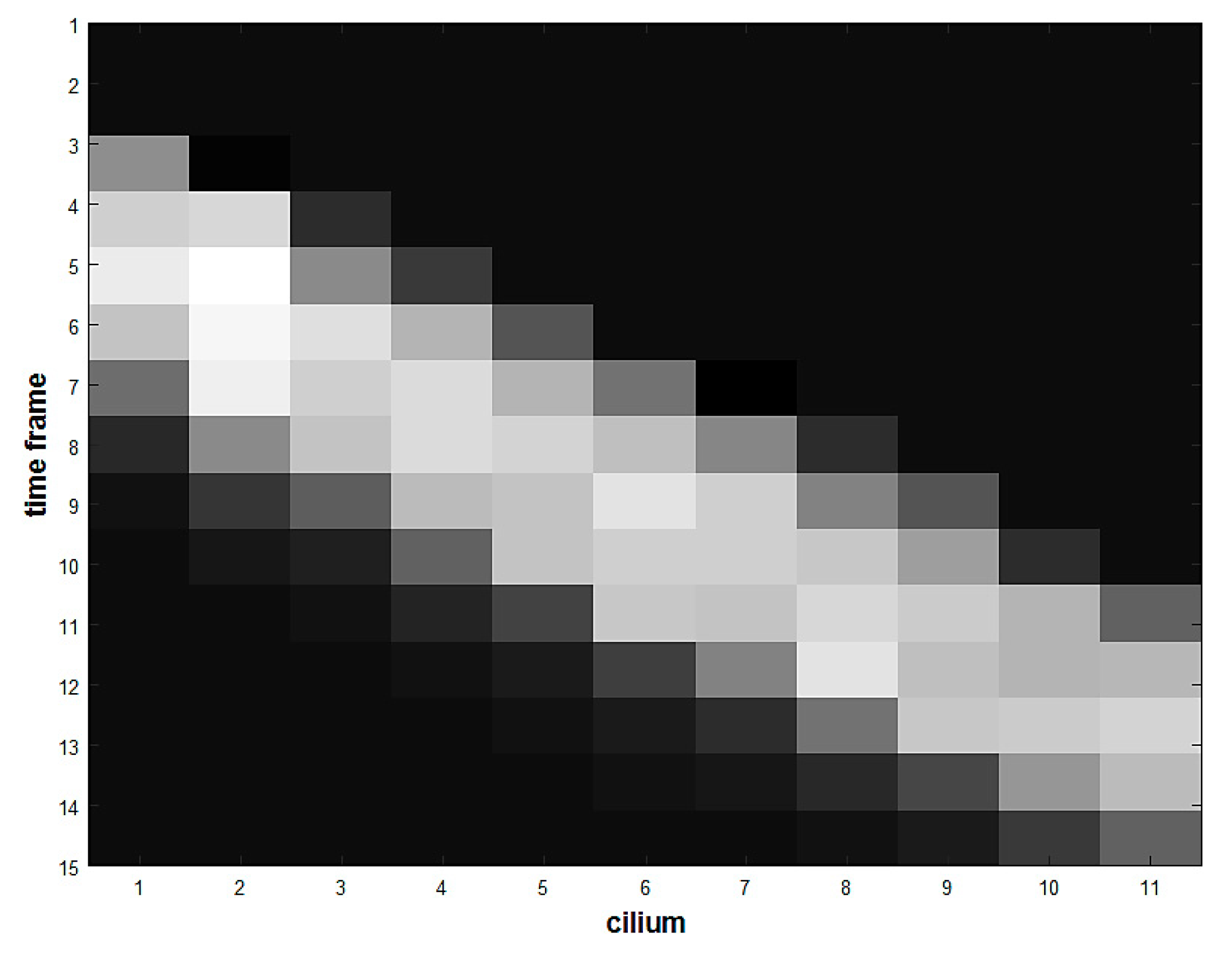
In order to move along the channel, the cell must bend the cilia. When the cilia bend, they generate stress at their bases. The value of the total force acting at the base of each of the 11 cilia is recorded every 0.2 s for 15 timeframes. After the cell passes through the ciliated section, therefore, we have 15 × 11 stress values that can be stored in a matrix F. If the force f is normalized according to
the normalized matrix F* can be seen as a greyscale image (Figure 9). Each cell produces a slightly different image according to its stiffness, size and initial position. This image represents a sort of fingerprint of the cell, and the ANN is trained to distinguish between soft and rigid fingerprints.
In all the simulations, I assume the two populations have the same average diameter d = 30 μm (±3 μm) and their only difference consists of their stiffness (and initial position). I consider three different cases where the stiffness of the two populations becomes gradually closer (Table 1).
The same ANN, with one hidden layer, is used in all three cases. The input layer has 165 nodes (the size of the matrix F*), the hidden layer has 3 nodes and the output layer has 1 node. All the layers are fully connected, and the logistic function is used as activation for all the nodes. The output of the ANN is the normalized stiffness
where k is the stiffness of the cell, and kmin and kmax are, respectively, the minimal and maximal stiffness of the set. The reader should not confuse the max. and min. stiffnesses in Table 1 and in Equation (6): the former are the maximal and minimal values of the population, the latter of the data set, which include instances of both populations.
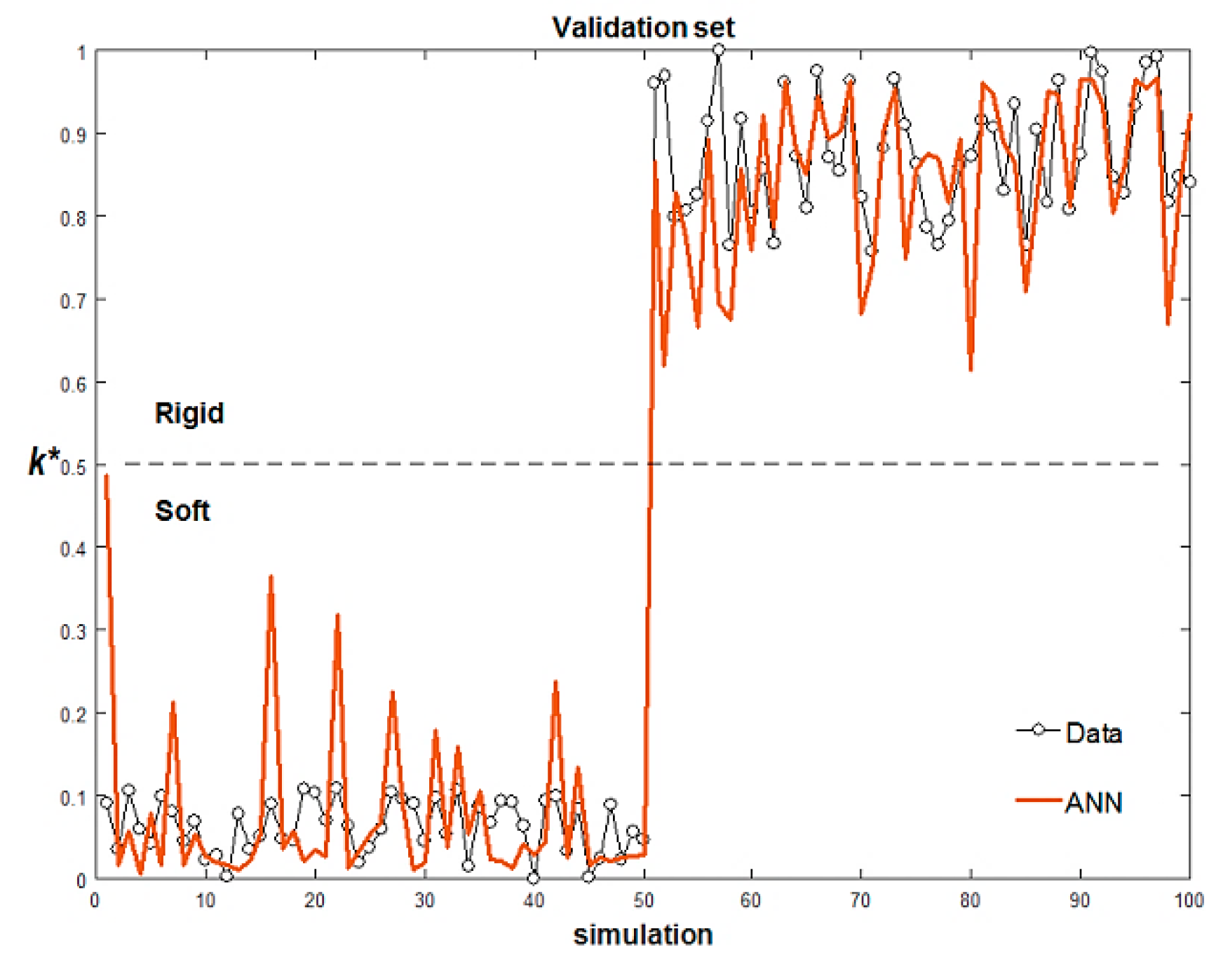
The training occurs together with the simulations in batch mode (batch size 100) for 1,000 epochs. Figure 10 shows the comparison between the data and the ANN output for both the training and the validation sets in case 1: when k* < 0.5, the cell is classified as soft; when k* > 0.5, the cell is classified as rigid.
When the difference in stiffness of the two populations is one order of magnitude (case 1 in Table 1), the ANN correctly identifies all the cells with 100% accuracy. In case 2, the stiffness of the rigid cells is only 2.5 times higher than that of the soft cells (Figure 11). The difference is lower than the previous case, but the model is still capable of distinguishing between the two populations with 100% accuracy. In case 3, the stiffness of the two populations only differs by 10%, and the stiffness of the two populations partially overlaps. The output of the ANN is reasonably accurate, and it fails to correctly classify only 11% of the cells.
After the neural component of the deep multiphysics model is trained, the model acquires the ability to separate cells with unknown stiffness (Figure 12). As a new cell moves into the device, the ANN reads the ‘stress fingerprint’ and classifies it as rigid or solid. In the first case, it opens the lower gate so the cell goes in the lower chamber; in the second case, it opens the upper gate, and the cell goes in the upper chamber. More details are given in the supplementary material: see the videos rigid_cell.avi and soft_cell.avi.
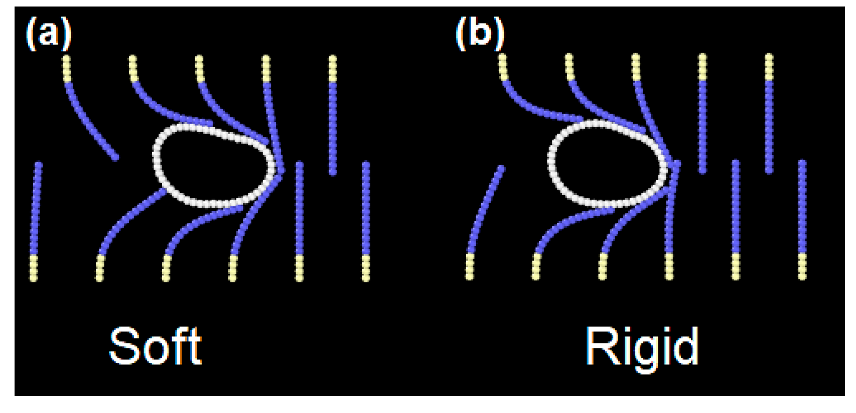
It is interesting to compare the performance of the model with respect to visual observation. Figure 12 shows two cells from case 1, where the stiffness difference is one order of magnitude. The different behaviour of the two cells can be clearly identified by visual observation. In case 3, in contrast, the cells stiffness is very close. As Figure 13 shows, visually the difference is minimal. However, the ANN is able to correctly separate the two cells in 89% of the cases.
6. Conclusions
There are two common ways of coupling FPM and ML. In one case, data are transferred from the ML algorithm to the FPM; in the other, from the FPM to the ML algorithm. In both cases, the coupling is in series: the two components remain distinct, and data generated by one model are subsequently fed into the other. This study introduces deep multiphysics; a computational framework that couples FPM and ML in parallel rather than in series. Deep multiphysics is based upon the concept of particle–neuron duality and only works with a particle-based FPM (discrete multiphysics) and a specific ML algorithm (ANNs) and, as a case study, it is applied here to the design of a microfluidic device for separating cell populations with different levels of stiffness.
A computational framework that couples FPM and ML in parallel can lead to computational methods that are well-grounded on the physics/chemistry/biology of the system under investigation but, at the same time, have the ability to ‘learn’ and ‘adapt’ during the simulation. In Alexiadis [5], a similar idea was applied to in-silico modelling of human physiology: DMP provided the physics of the system, while AI learned to replicate the regulatory intervention of the autonomic nervous system. This study generalizes that study by clearly defining the deep multiphysics framework and the particle–neuron duality.
This framework can lead to new ways of coupling first-principle modelling with AI. An idea, for instance, could be fluid neural networks: ANNs that are not organized within a fixed layered structure, but, similar to a fluid, change their local structure and connectivity with time. Additionally, the particle–neuron duality could also find application in swarm-intelligence, where agents, akin to particle–neuron hybrids, interact with each other following rules determined by (i) the (multi)physics of the environment and (ii) the information they exchange with each other.
Besides the applications mentioned above, there is an aspect of deep multiphysics that has deep theoretical implications. As discussed above, DMP combines particle methods such as SPH, LSM or DEM. The particle–neuron duality shows that, if we look at physical interactions as a form of information exchanged between particles, the mathematics behind these particle-methods and ANNs can be unified under the same computational paradigm. Within this paradigm, particle-based FPM (such SPH, LSM or DEM) and ANN-based ML algorithms are just two faces of the same coin: the AI algorithm does not need to be linked to the physical model anymore because the AI algorithm and the physical model are the same algorithm. One of the main conclusions of this work, therefore, is that, thanks to the particle–neuron duality, the coupling between ANNs and particle methods is more promising than the coupling of ANNs with mesh-based models. This study only scratches the surface of the possible implications of deep multiphysics, but, considering the recent upsurge of research activity dedicated to the coupling of FPM with ML, I believe it can have a far-reaching impact in the field.
Supplementary Materials
The following are available online at https://0-www-mdpi-com.brum.beds.ac.uk/2076-3417/9/24/5369/s1, video 1: rigid_cell.avi, video 2: soft_cell.avi.
Funding
This work was supported by the Engineering and Physical Sciences Research Council (EPSRC) grant number: EP/S019227/1.
Conflicts of Interest
The author declares no conflict of interest.
References
- Ibañez, R.; Abisset-Chavanne, E.; Aguado, J.V.; Gonzalez, D.; Cueto, E.; Chinesta, F. A Manifold Learning Approach to Data-Driven Computational Elasticity and Inelasticity. Arch. Comput. Methods Eng. 2016, 25, 1–11. [Google Scholar] [CrossRef] [Green Version]
- Snyder, J.C.; Rupp, M.; Hansen, K.; Müller, K.R.; Burke, K. Finding Density Functionals with Machine Learning. Phys. Rev. Lett. 2012, 108, 253002. [Google Scholar] [CrossRef] [PubMed]
- Zhang, Z.J.; Duraisamy, K. Machine Learning Methods for Data-driven turbulence modeling. In Proceedings of the 22nd AIAA Computational Fluid Dynamics Conference, Dallas, TX, USA, 22–26 June 2015. [Google Scholar]
- Liang, L.; Liu, M.; Martin, C.; Sun, W. A deep learning approach to estimate stress distribution: A fast and accurate surrogate of finite-element analysis. J. R. Soc. Interface 2018, 15, 20170844. [Google Scholar] [CrossRef] [PubMed] [Green Version]
- Alexiadis, A. Deep multiphysics: Coupling discrete multiphysics with machine learning to attain self-learning in-silico models replicating human physiology. Artif. Intell. Med. 2019, 98, 27–34. [Google Scholar] [CrossRef] [PubMed]
- Sutton, R.S.; Barto, A.G. Reinforcement Learning: An Introduction, 2nd ed.; MIT Press: Cambridge, MA, USA, 2018. [Google Scholar]
- Alexiadis, A. A smoothed particle hydrodynamics and coarse-grained molecular dynamics hybrid technique for modelling elastic particles and breakable capsules under various flow conditions. Int. J. Numer. Methods Eng. 2014, 100, 713–719. [Google Scholar] [CrossRef]
- Alexiadis, A. The Discrete Multi-Hybrid System for the simulation of solid-liquid flows. PLoS ONE 2015, 10, e0124678. [Google Scholar] [CrossRef] [PubMed] [Green Version]
- Ariane, M.; Allouche, M.H.; Bussone, M.; Giacosa, F.; Bernard, F.; Barigou, M.; Alexiadis, A. Discrete multiphysics: A mesh-free approach to model biological valves including the formation of solid aggregates. PloS ONE 2017, 12, e0174795. [Google Scholar] [CrossRef] [PubMed] [Green Version]
- Ariane, M.; Wen, W.; Vigolo, D.; Brill, A.; Nash, F.G.B.; Barigou, M.; Alexiadis, A. Modelling and simulation of flow and agglomeration in deep veins valves using Discrete Multi Physics. Comput. Biol. Med. 2017, 89, 96–103. [Google Scholar] [CrossRef] [PubMed]
- Ariane, M.; Vigolo, D.; Brill, A.; Nash, F.G.B.; Barigou, M.; Alexiadis, A. Using Discrete Multi-Physics for studying the dynamics of emboli in flexible venous valves. Comput. Fluids 2018, 166, 57–63. [Google Scholar] [CrossRef]
- Alexiadis, A.; Ghraybeh, S.; Qiao, G. Natural convection and solidification of phase-change materials in circular pipes: A SPH approach. Comput. Mater. Sci. 2018, 150, 475–483. [Google Scholar] [CrossRef]
- Alexiadis, A. A new framework for modelling the dynamics and the breakage of capsules, vesicles and cells in fluid flow. Procedia IUTAM 2015, 16, 80–88. [Google Scholar] [CrossRef] [Green Version]
- Rahmat, A.; Barigou, M.; Alexiadis, A. Deformation and rupture of compound cells under shear: A discrete multiphysics study. Phys. Fluids 2019, 31, 051903. [Google Scholar] [CrossRef]
- Rahmat, A.; Barigou, M.; Alexiadis, A. Numerical simulation of dissolution of solid particles in fluid flow using the SPH method. Int. J. Numer. Methods Heath Fluid Flow 2019. [Google Scholar] [CrossRef]
- McCulloch, W.S.; Pitts, W. A logical calculus of the ideas immanent to nervous activity. Bull. Math. Biophys. 1943, 5, 115–133. [Google Scholar] [CrossRef]
- Rosenblatt, F. The Perceptron: A Probabilistic Model for Information Storage and Organization In The Brain. Psychol. Rev. 1958, 65, 386–408. [Google Scholar] [CrossRef] [PubMed] [Green Version]
- Werbos, P. Beyond Regression: New Tools for Prediction and Analysis in the Behavioral Sciences; Harvard University: Cambridge, MA, USA, 1975. [Google Scholar]
Figure 1.
(a): Typical flow-chart of particle methods; (b): Internal forces used in Discrete Multiphysics (DMP).
Figure 1.
(a): Typical flow-chart of particle methods; (b): Internal forces used in Discrete Multiphysics (DMP).

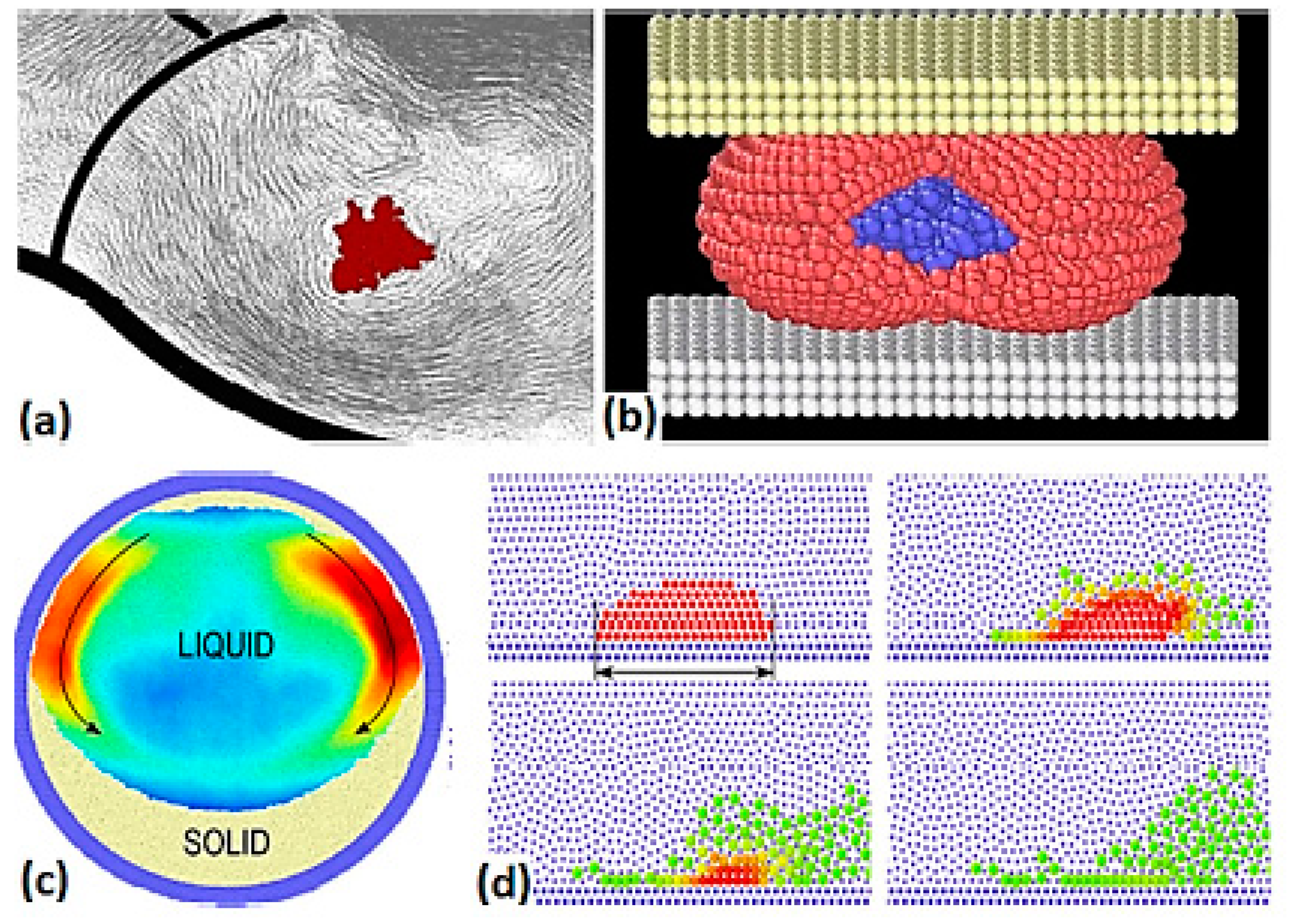
Figure 2.
Examples of applications of discrete multiphysics: cardiovascular flow (a), capsules breakup (b), phase transitions (c) and dissolution of solid particles (d).
Figure 2.
Examples of applications of discrete multiphysics: cardiovascular flow (a), capsules breakup (b), phase transitions (c) and dissolution of solid particles (d).

Figure 3.
(a): A single artificial neuron; (b): An example of a (deep) artificial neural network with two hidden layers.
Figure 3.
(a): A single artificial neuron; (b): An example of a (deep) artificial neural network with two hidden layers.

Figure 4.
(a): Solid and fluid particles exchange mechanical forces; (b): Hot and cold particles exchange heat; (c): Layers of neurons exchange information.
Figure 4.
(a): Solid and fluid particles exchange mechanical forces; (b): Hot and cold particles exchange heat; (c): Layers of neurons exchange information.

Figure 5.
Mutual relations between ‘forces’ and discrete mechanics, ‘interactions’ and discrete multiphysics, and ‘information’ and deep multiphysics.
Figure 5.
Mutual relations between ‘forces’ and discrete mechanics, ‘interactions’ and discrete multiphysics, and ‘information’ and deep multiphysics.

Figure 6.
The concept of the proposed microfluidic separator.

Figure 7.
Schematic representation of the particle types used in the simulations.

Figure 8.
Deep multiphysics model of the separation device. The number of neurons/layers is not representative of the actual Artificial Neural Network (ANN) used but is only for illustrative purposes.
Figure 8.
Deep multiphysics model of the separation device. The number of neurons/layers is not representative of the actual Artificial Neural Network (ANN) used but is only for illustrative purposes.

Figure 9.
The ‘stress’ fingerprint of a cell with stiffness k = 4.5 × 10⁻¹⁵ J.

Figure 10.
(a): Comparison between data and the ANN results for both the training and (b): The validation sets in case 1. In both cases, the first 50 simulations refer to cells from the soft population and the other 50 from the rigid population.
Figure 10.
(a): Comparison between data and the ANN results for both the training and (b): The validation sets in case 1. In both cases, the first 50 simulations refer to cells from the soft population and the other 50 from the rigid population.

Figure 11.
Comparison between data and the ANN results for both the validation sets in case 2.

Figure 12.
The final deep multiphysics model in action (a): rigid cell; (b): soft cell.

Figure 13.
(a): soft cell; (b): rigid cell in case 3.


Table 1.
Minimal, average and maximal stiffness of the two populations for the three cases considered. Err is the percentage of soft cells erroneously classified as rigid by the ANN, and vice versa, in the validation set.
Table 1.
Minimal, average and maximal stiffness of the two populations for the three cases considered. Err is the percentage of soft cells erroneously classified as rigid by the ANN, and vice versa, in the validation set.
| k Soft Population [J∙1015] | k Rigid Population [J∙1015] | ||||||
|---|---|---|---|---|---|---|---|
| Case | Min. | Ave. | Max | Min. | Ave. | Max | Err % |
| 1 | 1.8 | 2 | 2.2 | 18 | 20 | 22 | 0 |
| 2 | 3.6 | 4 | 4.4 | 9 | 10 | 11 | 0 |
| 3 | 4.05 | 4.5 | 4.95 | 4.5 | 5 | 5.5 | 11 |
© 2019 by the author. Licensee MDPI, Basel, Switzerland. This article is an open access article distributed under the terms and conditions of the Creative Commons Attribution (CC BY) license (http://creativecommons.org/licenses/by/4.0/).
Share and Cite
MDPI and ACS Style
Alexiadis, A. Deep Multiphysics and Particle–Neuron Duality: A Computational Framework Coupling (Discrete) Multiphysics and Deep Learning. Appl. Sci. 2019, 9, 5369. https://0-doi-org.brum.beds.ac.uk/10.3390/app9245369
AMA Style
Alexiadis A. Deep Multiphysics and Particle–Neuron Duality: A Computational Framework Coupling (Discrete) Multiphysics and Deep Learning. Applied Sciences. 2019; 9(24):5369. https://0-doi-org.brum.beds.ac.uk/10.3390/app9245369
Chicago/Turabian StyleAlexiadis, Alessio. 2019. "Deep Multiphysics and Particle–Neuron Duality: A Computational Framework Coupling (Discrete) Multiphysics and Deep Learning" Applied Sciences 9, no. 24: 5369. https://0-doi-org.brum.beds.ac.uk/10.3390/app9245369
Note that from the first issue of 2016, this journal uses article numbers instead of page numbers. See further details here.