Efficient Parallel Algorithms for 3D Laplacian Smoothing on the GPU


1
School of Engineering and Technology, China University of Geosciences (Beijing), Beijing 100083, China
2
Airport Engineering Civil Aviation R&D Base, China Airport Construction Group Co., Ltd., Beijing 100621, China
3
China Super-Creative Airport Technical Co., Ltd., Beijing 100621, China
*
Authors to whom correspondence should be addressed.
Appl. Sci. 2019, 9(24), 5437; https://0-doi-org.brum.beds.ac.uk/10.3390/app9245437
Submission received: 13 November 2019
/
Revised: 6 December 2019
/
Accepted: 6 December 2019
/
Published: 11 December 2019
(This article belongs to the Special Issue Computational Methods for Fracture Ⅱ)
Abstract
:In numerical modeling, mesh quality is one of the decisive factors that strongly affects the accuracy of calculations and the convergence of iterations. To improve mesh quality, the Laplacian mesh smoothing method, which repositions nodes to the barycenter of adjacent nodes without changing the mesh topology, has been widely used. However, smoothing a large-scale three dimensional mesh is quite computationally expensive, and few studies have focused on accelerating the Laplacian mesh smoothing method by utilizing the graphics processing unit (GPU). This paper presents a GPU-accelerated parallel algorithm for Laplacian smoothing in three dimensions by considering the influence of different data layouts and iteration forms. To evaluate the efficiency of the GPU implementation, the parallel solution is compared with the original serial solution. Experimental results show that our parallel implementation is up to 46 times faster than the serial version.
1. Introduction
Numerical simulation is the most popular method for studying engineering and physical problems, and the finite element method (FEM) is the most widely developed and mature method. However, the accuracy of FEM simulation results is dominated by the quality of the mesh. This is not only because the mesh is the basis of discretization, but also because of the poor condition of stiffness matrices caused by poor mesh. To obtain a high quality mesh, many mesh generation methods have been proposed [1]. The original mesh generated by those improved methods then needs further optimization. Mesh clean-up and mesh smoothing are the two major categories of optimization. The former improves the mesh quality by changing the original topology [2,3], such as by encryption and reordering [4]. Mesh smoothing, which relocates vertices to improve the mesh quality, is a simpler method and retains the mesh topology [5,6,7]. Laplacian smoothing is a commonly used mesh smoothing methods that moves nodes in the mesh to the geometric center of the adjacent nodes [8]. Laplacian smoothing is easy to implement and use because it does not require other complex operations. Various versions of Laplacian smoothing have been developed to improve the performance of the original form of Laplacian smoothing [9,10,11].
However, when dealing with complex meshes consisting of a large number of nodes and elements, the computation is usually expensive due to the iteration process. To improve the efficiency of smoothing, parallel computing is introduced as an effective strategy [12]. The parallel implementation of Laplacian smoothing has been developed with the computational power of modern multi-core central processing unit (CPU) and GPU.
For example, Jiao et al. [13] developed a parallel mesh smoothing algorithm for curved surface meshes that can retain the original features of the mesh. It was implemented on 128 processors of distributed storage computers. Sastry and Shontz [14] proposed a new parallel method to untangle log-barrier meshes and improve their quality with the help of an open message passing interface (OpenMPI). The experimental results show that the execution time fluctuates within a certain range when the size of the mesh is proportional to the number of processors executing the algorithm. Cebrián et al. [15] proposed an efficient code modernization strategies to 3-D Stencil-based applications while the use of aligned data layout and the dynamic parallel policy can significantly improve the performance. Titarenko and Hildyard [16] presented a new approach for parallelisation of a finite difference code on a single processor. The rearranging of data structure can be a useful strategy in utilizing vectorisation. Sangeet Dahal and Timothy S. Newman [17] developed an efficient smoothing method for 2D meshes on a GPU and the GPU algorithm has a speedup of 10 to 50 times. Benitez [18] proposed a highly scalable algorithm for tetrahedral meshes derived from a sequential mesh optimization method. Hernández et al. [19] analyze the programmability, performance and energy using a 3-D Finite Difference implementation to evaluate the efficiency of different massively parallel architectures. The benchmark tests results show the parallel implementation developed on Maxwell GPU is the most power efficient accelerator which provides the direction of future study. D’Amato and Venere [20] proposed a heterogeneous computing method to optimize the quality of large-scale meshes. The algorithm first determines a possible moving position near the smooth node and then determines the optimal position by evaluating the quality of the moving mesh. By distributing the elements in multiple threads, it avoids the use of lock strategies and possible data access conflicts.
Most recently, Mei et al. [21] presented a more general paradigm for the two major iteration forms of Laplacian smoothing. Two special compute unified device architecture (CUDA) kernels were designed to solve the race condition in neighbor search and data dependence in smooth iteration. Experimental results have indicated that Form A, which needs to swap intermediate nodal coordinates is always slower than the form that does not swap data. Zhao et al. [22] further optimized the smart Laplacian smoothing algorithm with the help of CUDA dynamic parallelism. This nested CUDA code can greatly simplify the comparison of mesh quality so that the iteration process can be optimized. However, because a parent core needs to call two subcores, the performance of parallel computing is not fully utilized, which results in this version being slightly faster than the original GPU version.
It is remarkable that most of the above studies focused on two dimensional cases. However, it is obvious that mesh composed of tetrahedrons or hexahedrons is more suitable for various kinds of numerical simulations. Therefore, a parallel solution for Laplacian smoothing in three dimensional applications is necessary.
This paper presents an efficient three dimensional Laplacian smoothing based on GPU acceleration. With the help of parallel sort and unique, we search and store the first-order neighbors in the subarea to avoid conflicts. The effects of different data structures are also considered, including the array of non-aligned structures, array of aligned structures, and structure of arrays. In addition, new iteration kernels have been designed, which make full use of the power of the GPU and thus significantly reduce the number of iterations.
The rest of paper is organized as follows. Some basic concepts and principles of Laplacian smoothing and data layout is given in Section 2. The next Section 3 presents some key issue and implementation details of 3D parallel Laplacian Smoothing. Section 4 and Section 5 mainly elaborate on the results of several groups of experimental tests and the discussion of GPU acceleration performance of each part. Finally, in Section 6 we present our conclusions.
2. Background
2.1. Laplacian Mesh Smoothing
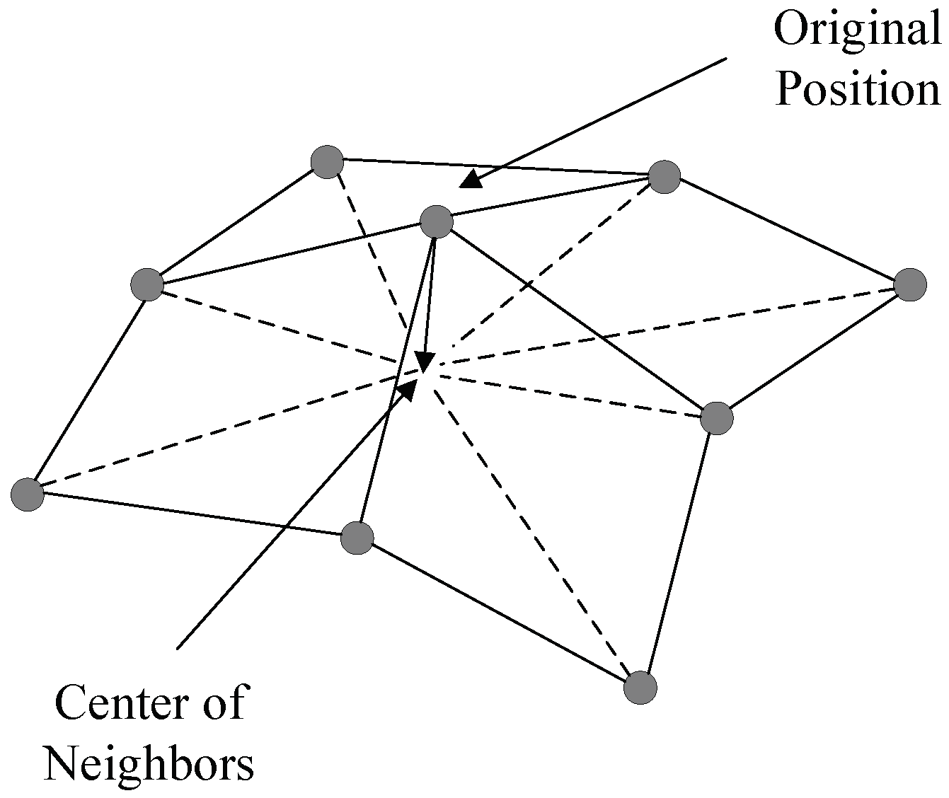
Mesh smoothing is one of the most important methods for improving the quality of a mesh by adjusting the location of nodes in the mesh while keeping the topology of the mesh unchanged. Laplacian smoothing is one of the most basic and common method. The core idea of Laplacian smoothing is to reposition each node to the centroid of its first-order neighboring nodes; see Figure 1. On the basis of Laplacian smoothing, many improved versions such as Taubin [11], weighted Laplacian smoothing [9,23], smart Laplacian smoothing [10,24] and HCLaplacian [25], have been developed.
2.2. Iteration Forms
Two forms of Laplacian smoothing are proposed to select the coordinates of the neighboring nodes during the smoothing process. Form A selects the old coordinates calculated in the previous pass while Form B uses the new coordinates that have been calculated in the current iteration; see the following formulations.
Form A:
where N is the number of neighbors of node i, and is the new coordinate after smoothing in next pass (q + 1).
Form B:
where N is the number of neighbors of node i, and is the new position of node i in the next pass (q + 1). and are the numbers of neighbors derived from passes q and (q + 1), respectively. Form A is clearly a special case of the Form B where .
2.3. Data Layouts in Memory
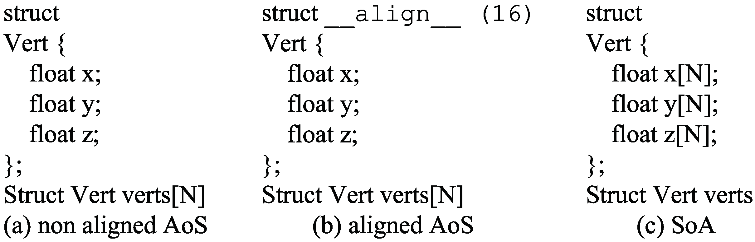
Data structures are usually divided into two types, whether in CUDA or any similar architecture, array of structures (AoS) and structure of arrays (SoA) forms [26]. The choice of AoS or SoA for optimal performance usually depends on access patterns. Usually, the use of non-aligned AoS data structures leads to coalescing issues while SoA structures will certainly be aligned. In general, it is more convenient to use the structure-of-arrays in CUDA and single instruction multiple data (SIMD) programs. However, we will compare the performance of these forms in the following applications; see Figure 2.
3. GPU-Accelerated Parallel Algorithm for 3D Laplacian Smoothing
3.1. Procedure of the Algorithm
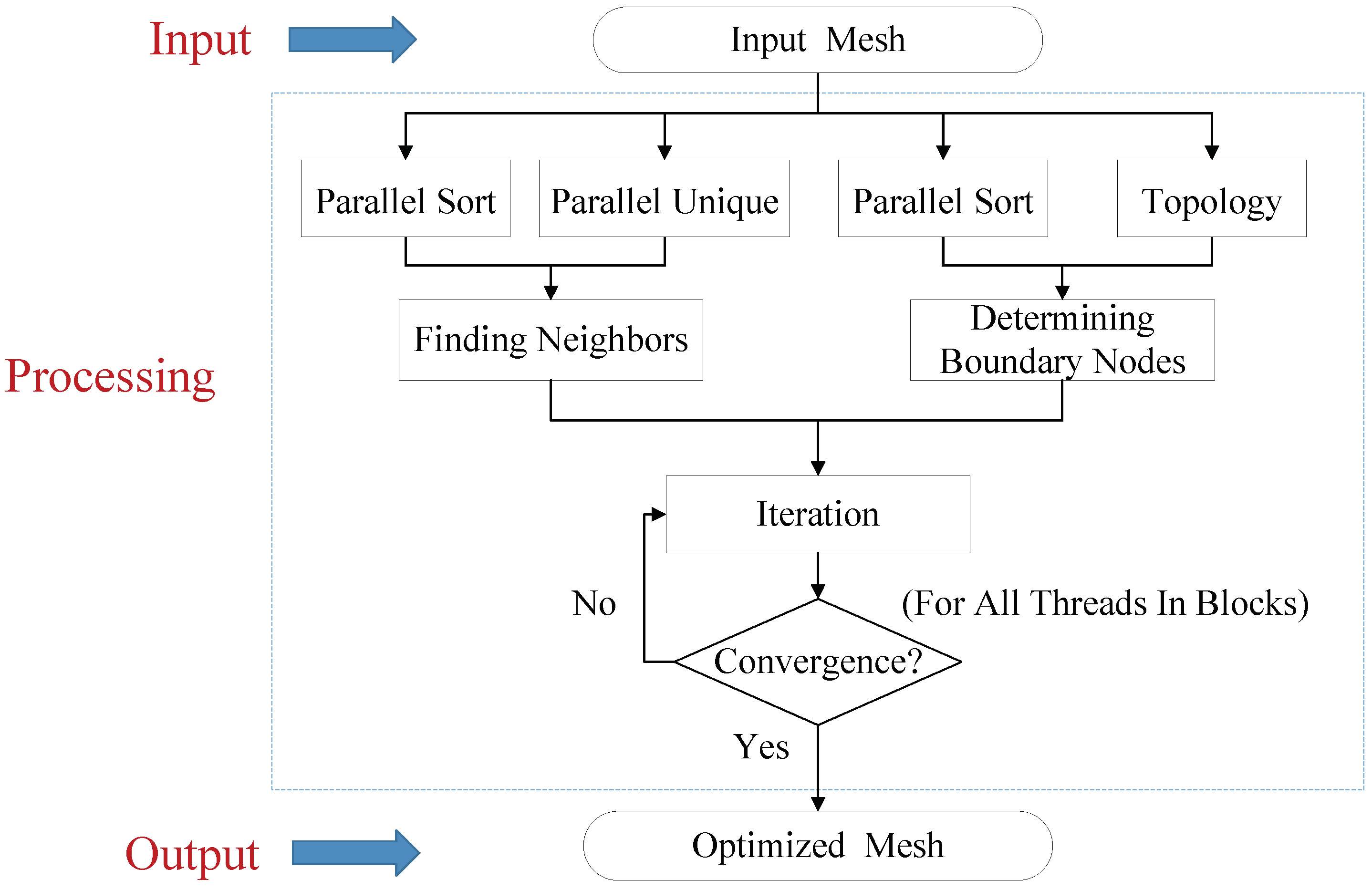
As mentioned above, we divide the Laplacian smooth workflow into three subprocedures. The first step is to find the first-order domain of each node so that their geometric center can be determined. The shape and volume of mesh models are major features that should be preserved. As a result, the boundary points will be constrained, and only the interior points will be smoothed, which is the work of the second subprocess. Finally, the iteration process calculates the position of the smoothing node until convergence. The overall workflow is illustrated in Figure 3.
3.2. Details and Key Issues of the Parallel Algorithm
3.2.1. Finding Neighbors
Since the new positions of smooth nodes depend on the coordinates of their first-order neighbors, they must be found first. Generally, the first-order neighbors of a node are determined by the spatial topological relationship of the mesh in which the node is located. For a tetrahedron, any node is the neighbor of the other three nodes.
A simple and clear method is to allocate an array to store the neighbors in the node structure, and then search each tetrahedron in the mesh in turn [21]. However, since the number of neighbors for each node is unknown, we can only allocate the memory of the neighbor array step by step in the kernel function. This potentially creates data conflicts for the writing operations; it is likely that more than one thread will write a neighbor of a node to the same element of the array at the same time (i.e., the same memory address). In addition, due to the existence of variable-size arrays in such data structures, sorting and other operations will fail in subsequent implementations.
A feasible method is to change the storage structure of neighbors [27]. We use edges as basic units to store neighbor information. The process of finding the first-order neighbors for each node is as follows.
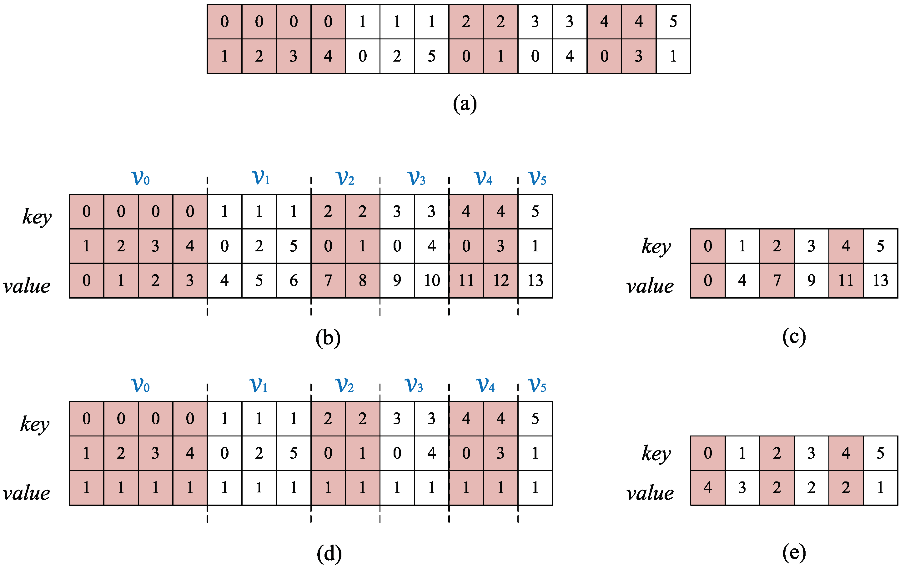
First, all edge sets are copied in reverse order and sorted according to the IDs of node A and then node B so that all the edges with the same node A are listed in succession. These edge sets constitute the neighbors of a particular node. In this way, the index of each neighbor can be determined by the head pointer or length of each segment. The head pointer can be obtained by performing a unique operation. The length can be easily obtained by calculating the distance between each pointer. The essential ideas are illustrated in Figure 4.
With the help of the CUDA thrust library [28], these unique operations can be easily parallelized; then, the head positions of all segments can be obtained, and another parallel primitive is invoked to calculate the lengths of all segments in parallel. Finally, a CUDA kernel is designed to write the header pointers and the number of the neighbor into memory.
3.2.2. Determining Boundary Nodes
Constraint points are used to guarantee the overall topological characteristics of the mesh in the smoothing process. In this implementation, we use boundary points as constraint points.
In a planar mesh, a point can be judged as a boundary point by checking its neighbors. Similarly, the boundary points in three dimensional space can be judged by the relationships of the mesh structure, except that the basic elements are faces rather than edges. The basic idea is that if a face is used twice in the spatial mesh, it must be an internal surface and the point on it must be an internal point, while boundary points are the points on surfaces that are used only once.
The process of determining boundary nodes is as follows:
- Loop over all elements and store node indices representing their four faces from small to large;
- Sort the surface array so that any surface can be compared with its adjacent surface to determine whether it has been used only once (i.e., boundary face);
- Run a CUDA kernel to record points on the boundary surfaces and set them as constraints.
3.2.3. Iteration Procedure
Laplacian smoothing is an iterative procedure. Unlike the serial implementation of it, the parallel version requires iterative computation of a series of nodes at the same time. It must be ensured that the previous iteration is completed before the new iteration begins, and the smoothing process will use the updated coordinates. Therefore, it is necessary to set a barrier at the end of each iteration.
In CUDA, this kind of data dependence within a single block can be easily solved by using the barrier __syncthreads(). However, synchronization between all blocks is not designed in CUDA because it consumes a lot of GPU operations and has low returns. A feasible solution is to allocate only one block for iteration, so that each iteration is completed before the next step.
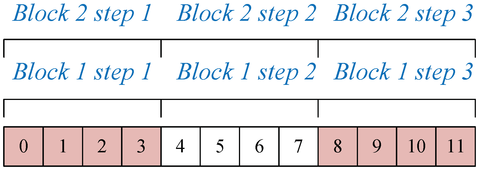
Clearly, using only one block effectively avoids data collision, but it does not exploit the GPU efficiently. Note that in Laplacian smoothing, the current iteration pass always converges regardless of whether the coordinates of points are updated, and the results remain unchanged. Therefore, we adopted a new form using multiple blocks; see Figure 5.
In this case, different blocks iterate over the same part of the node together, even though the coordinates of the nodes they use are not consistent. Blocks that launch earlier use old values, while those that start later use updated values. The result is always computed towards the end of the iteration. As the iteration proceeds, more and more blocks converge and exit the computation until the last block completes the iteration.
4. Results
4.1. Experimental Environment and Testing Data
Five groups of three dimensional meshes are generated as experimental data, with a number of points from 5k to 100k. First, a user-specified cube is determined, and the nodes are distributed equidistantly on it; then, nodes are generated randomly in this spatial range; finally, Delaunay meshes consisting of these discrete point sets are created using TetGen library [29]. In addition, we also test a slope model with 77k nodes as a supplement.
These parallel solution tests are performed on a workstation computer. The specifications of the workstation are listed in Table 1.
4.2. The Running Time and Speedup of Form A in Standard Laplacian smoothing
4.3. The Running Time and Speedup of Form B in Standard Laplacian Smoothing
5. Discussion
5.1. Evaluation of Our Algorithm
5.1.1. Performance of Parallel Method of Finding Neighbors
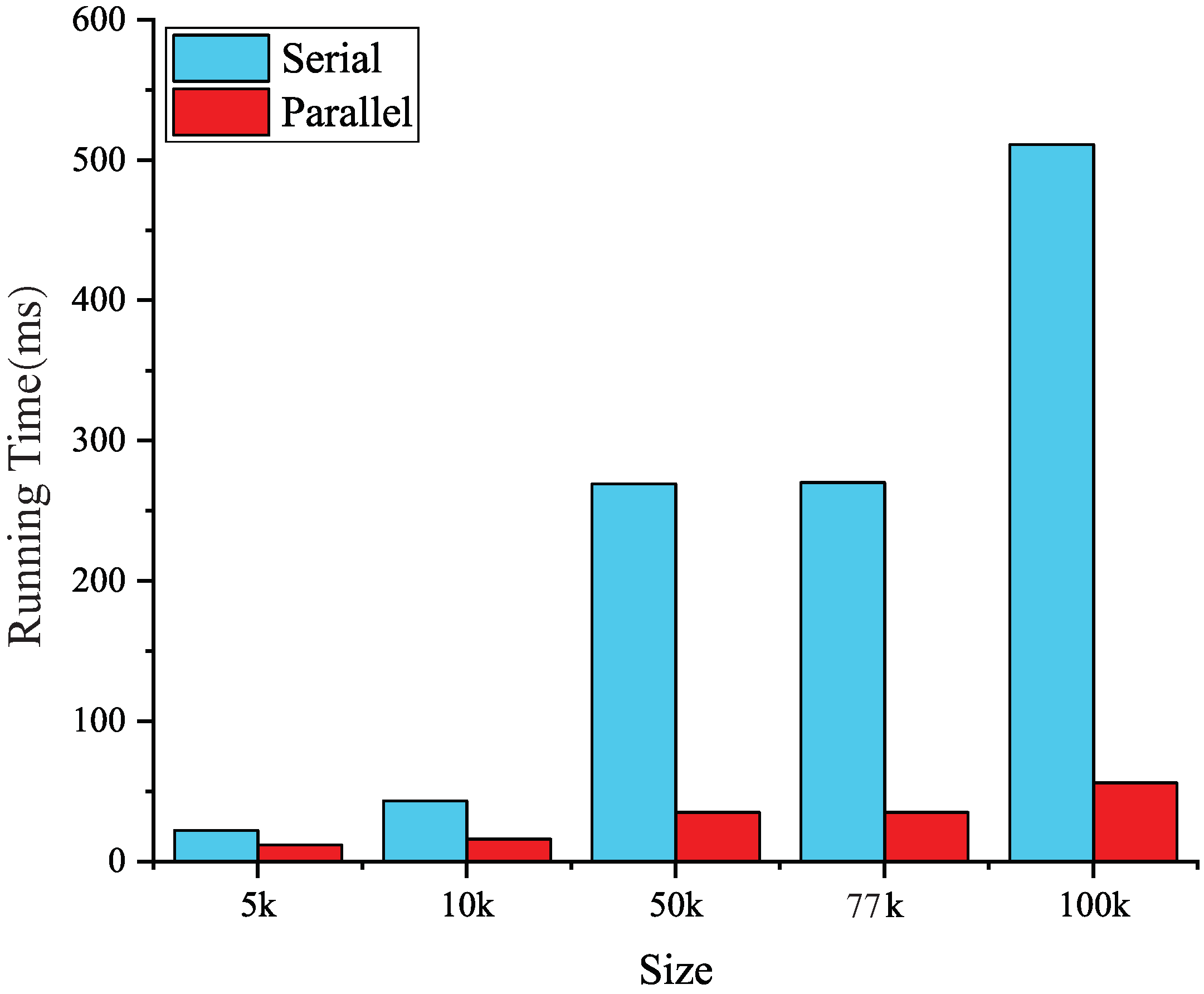
The method we use to find the first-order neighborhood is easy to implement. Unlike mesh coloring, one of the most popular methods for dealing with race condition issues, it only needs a handful of kernels to complete data transmission, while the other parts of the algorithm are implemented by thrust library without much additional code.
As mentioned in Section 3.2.1, an auxiliary array of sequenced integers is allocated to determine the head pointer of each neighbor’s segment. Then, a parallel scan is implemented with the help of thrust::unique_by_keys(). After eliminating the edges of the same first node, the indices of neighbors can be easily obtained. Similarly, an auxiliary array is created to quickly calculate the length of each segment; then, the primitive thrust::reduction_by_keys() is used to collect all edges in the same segment; finally, both the head pointer and the number of each node are obtained and stored in the corresponding array.
This significantly improves the efficiency of implementation; see Figure 6.
5.1.2. Impact of Data Layouts
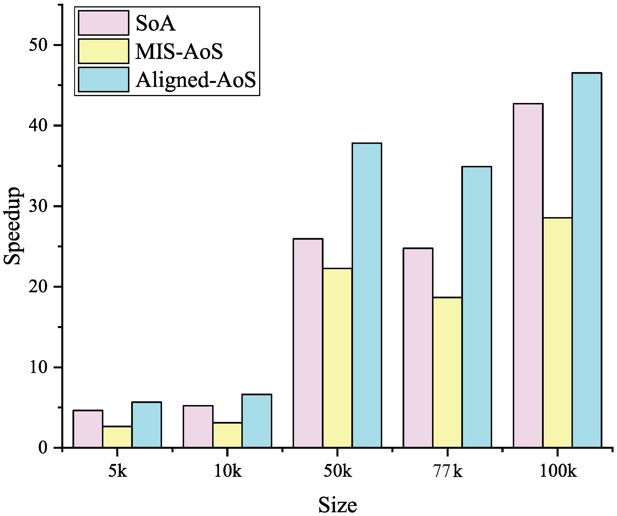
Figure 7 shows the speedups for different data layouts. This indicates that non aligned AoS is the slowest and SoA performs better while the aligned version of AoS is the best. This behavior is mainly due to the coalesced memory accesses. Note that the alignment specifier __align__() in CUDA works only when the structure size is less than 16 bytes since there are more than one global memory access cannot be merged while beyond this upper limit. Aligned AoS may be the best data layouts in this implementation, but it is usually easier to achieve rapid speedup using SoA.
5.1.3. Different Iteration Forms
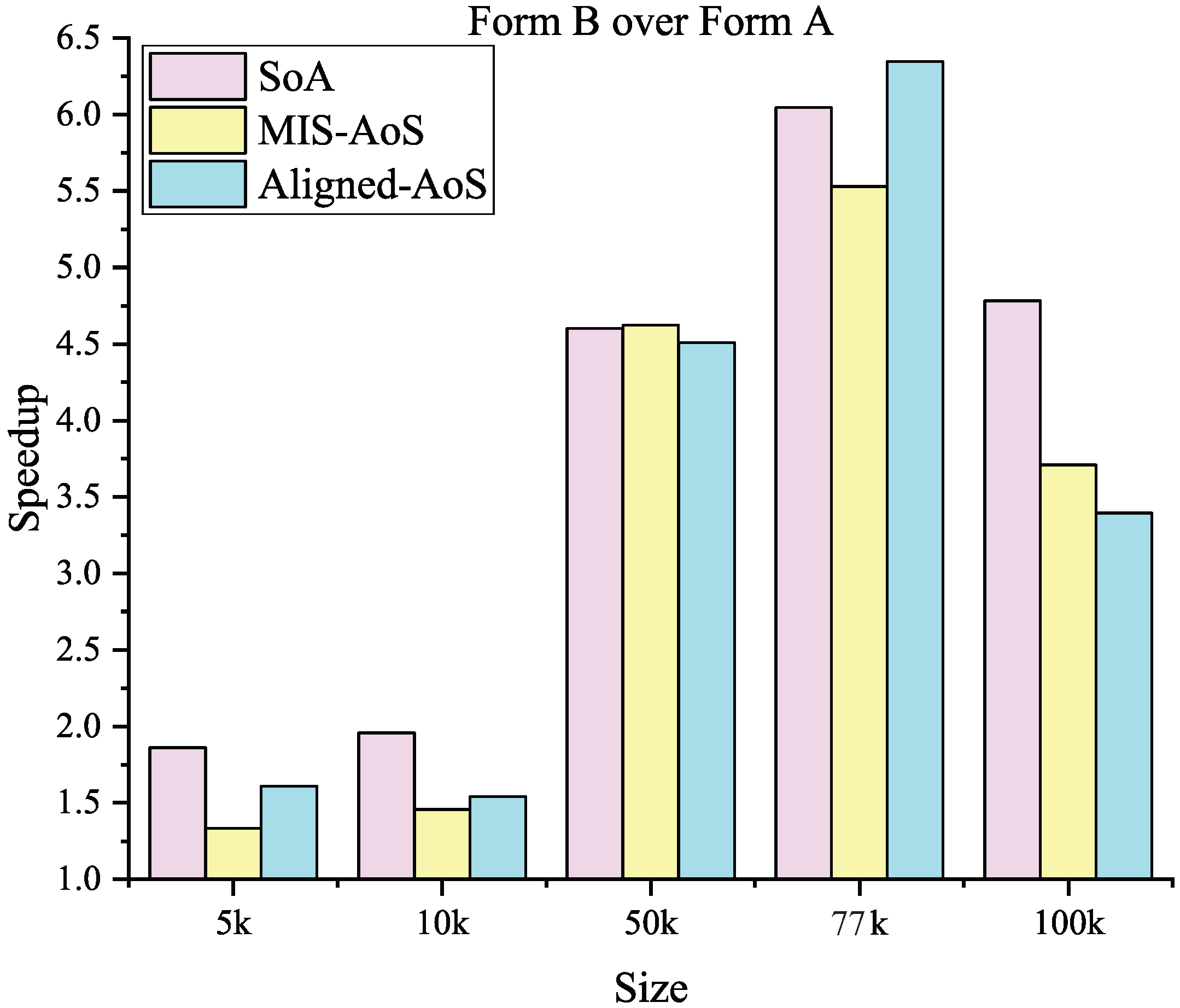
According to the results, Form B Laplacian smoothing is always faster than Form A which needs to update node coordinates immediately in its iterations; see Figure 8.
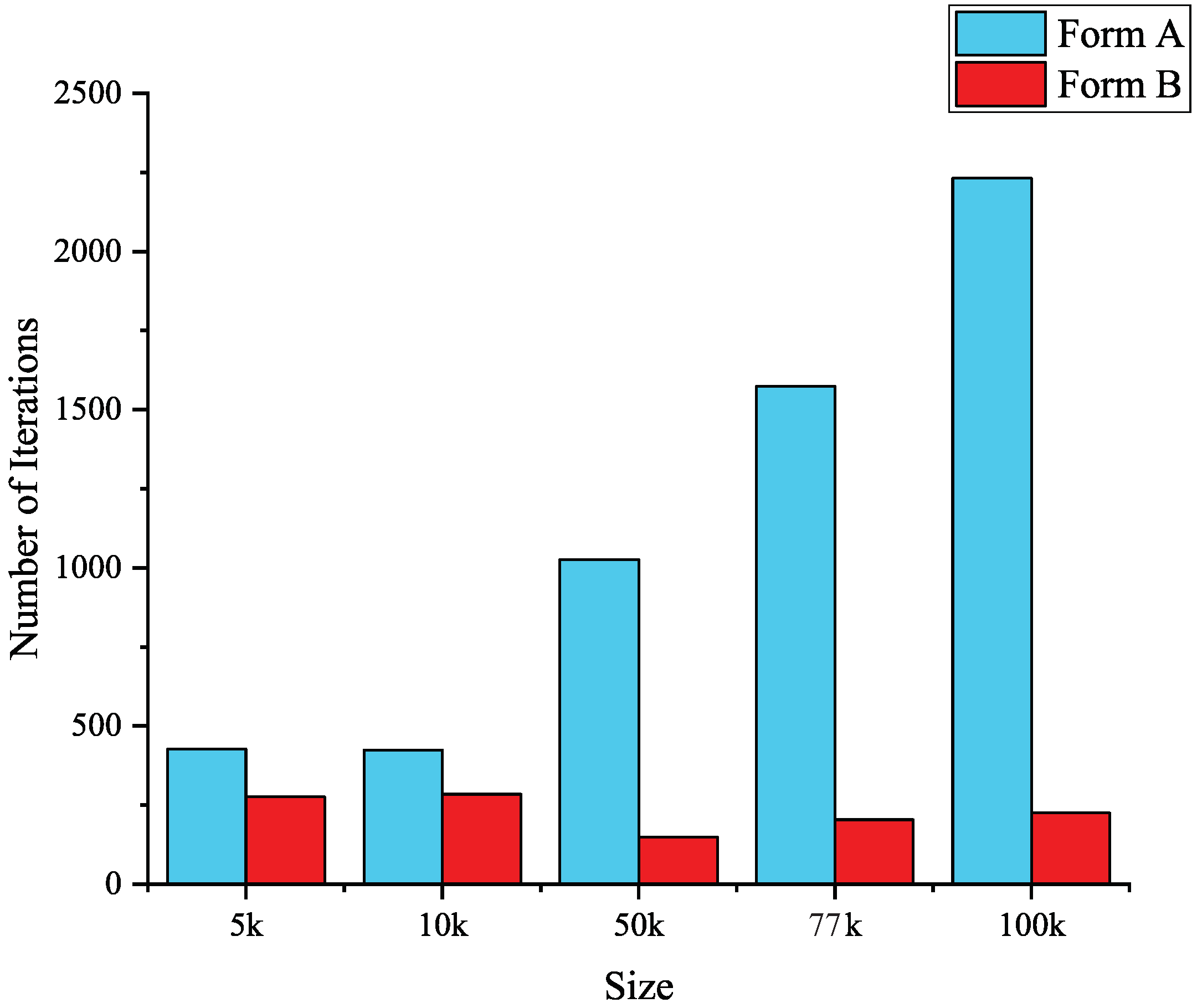
There are two possible reasons for this performance. First, Form A requires data exchange, which means more memory for storing new coordinates and more frequent global memory access. Global memory is the largest and most commonly used memory in the GPU, but it also has the highest latency compared with other memory. Too much global memory access reduces throughput efficiency. The other reason is that Form A updates the coordinates of smooth nodes immediately after each iteration, which makes the calculation more accurate and reasonable in theory. However, it does not significantly improve accuracy but leads to an increase in the number of iterations. Figure 9 shows the number of convergences for both iteration forms; it can be seen that the larger the scale of the test data, the greater the number of convergences of Form A compared with Form B. As a result, it is wise to use Form B in practice.
5.1.4. Analysis of the Improvement of Iterative Convergence Speed
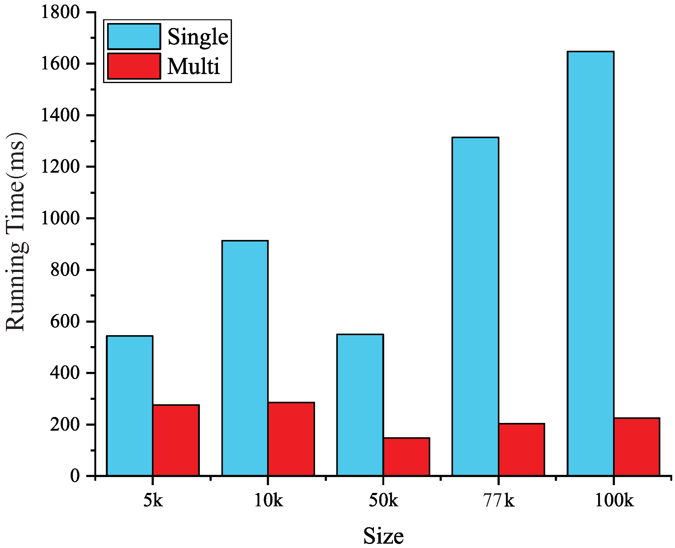
The iteration procedure dominates most of the running time. Therefore, accelerating the speed of iteration convergence is the core task to improve the efficiency of the algorithm. Data dependence is the main problem that needs to be solved. Using thread synchronization is an effective solution to this problem. However, because it is limited by the current GPU architecture, a block contains a maximum of 1024 threads; that is to say, the old solution only allows 1024 threads to participate in the calculation at the same time, which is less than the usual number of simultaneous calls by the GPU.
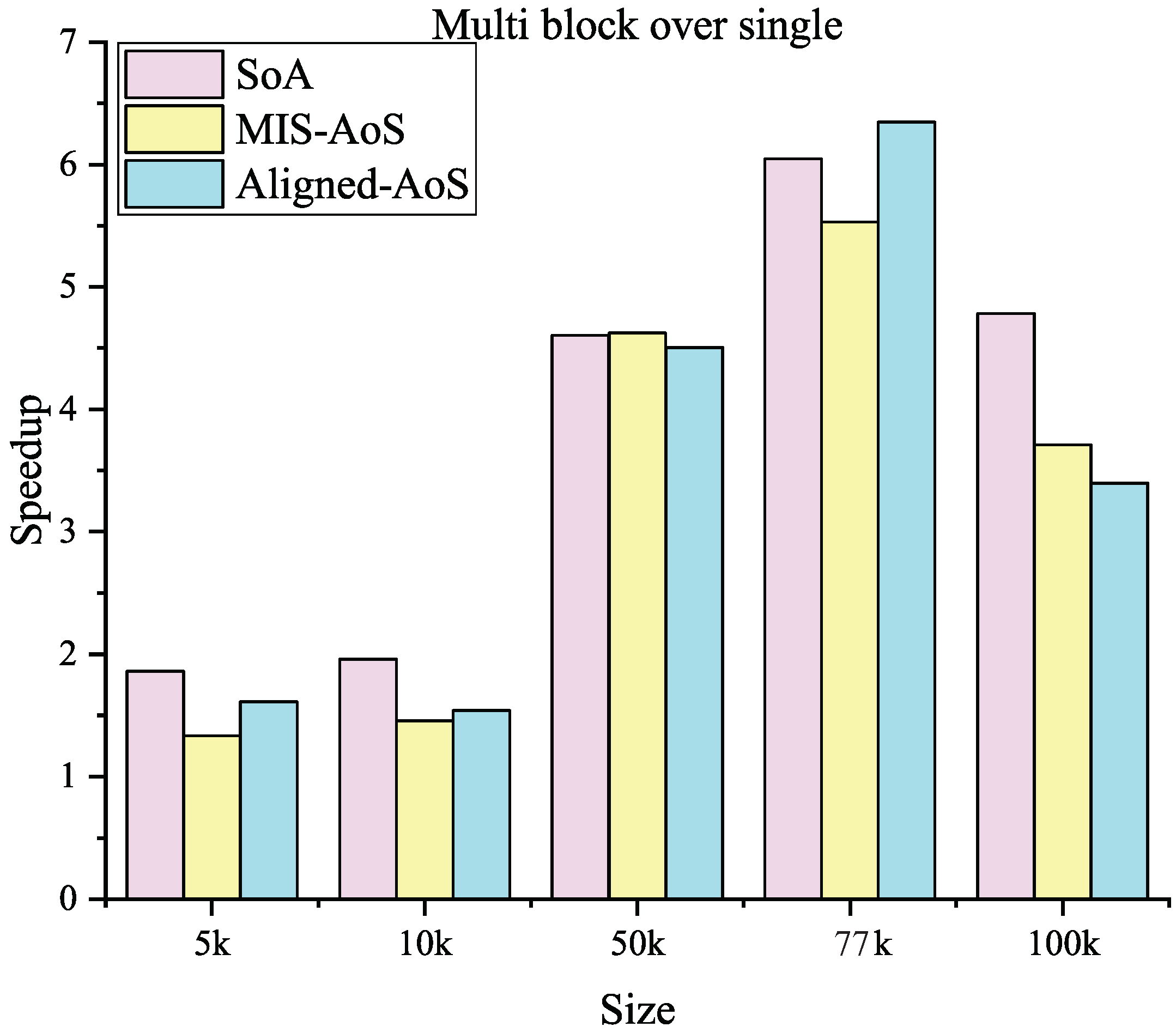
As mentioned in Section 3.2.3, a new kernel with multiple blocks is designed to compute the smoothing process of the same set of nodes to make the iteration more efficient. Even though the data used in the iteration may be duplicate, the interleaving operations make each thread converge faster and precisely as well. First, the iteration times for multiple blocks are a great deal less than for a single one; see Figure 10. Moreover, the final result is close to or even equal to the true value (i.e., the error is less than 0.0001). In any case, as shown in Figure 11, this version runs 2∼6 times faster.
5.2. Outlook
Laplacian smoothing is a simple and common mesh optimization method. Because of its simple theory, it is easy to create inverted or even invalid elements when dealing with high concave areas. However, it is this simplicity that makes its operation efficient and timesaving, making it still the most popular method. Compared with other optimization algorithms, its speed advantage is quite obvious. Additionally, other optimized versions of Laplacian smoothing do not significantly increase running time while improving smoothness based on curvature or preventing the overall shrinkage of the model. Therefore, these versions are also worth exploring in the future.
6. Conclusions
In this paper, we have presented an efficient parallel Laplacian smoothing algorithm in three dimensions using GPU acceleration. Two different iteration methods and three data layouts are employed to implement the parallel algorithm. We have also designed a parallel method to find first-order neighbors while avoiding potential race condition problems. A novel iteration kernel is implemented to optimize GPU utilization while solving the problem of data dependence. Five groups of benchmark tests show that the speedup of GPU implementation reaches 46×. They also indicate that the data structure SoA is nearly 1.5 times faster than non-aligned AoS while the aligned version of AoS achieves the best efficiency. Iteration Form A requires more data exchange, which results its spending more time on global memory access. In the long run, it is always slower than Form B. Moreover, by using a special strategy, allocating multiple blocks does not cause data dependence problems and makes it easy for the iterations to converge.
Author Contributions
Conceptualization, L.X., G.M., G.Y.; Methodology, L.X., G.Y., G.M., K.Z.; Writing-Original Draft Preparation, L.X., G.M.; Writing-Review & Editing, L.X., G.Y., G.M., K.Z.
Funding
This research was jointly supported by the National Natural Science Foundation of China (Grant No. 11602235), and the Fundamental Research Funds for China Central Universities (Grant Nos. 2652018091, 2652018107, and 2652018109).
Acknowledgments
The authors would like to thank the editor and the reviewers for their contributions.
Conflicts of Interest
The authors declare no conflict of interest.
Abbreviations
The following abbreviations are used in this manuscript:
| GPU | Graphics Processing Unit |
| FEM | Finite Element Method |
| CPU | Central Processing Unit |
| OpenMPI | Open Message Passing Interface |
| CUDA | Compute Unified Device Architecture |
| SoA | Structure-of-Arrays |
| AoS | Array-of-Structures |
| SIMD | Single Instruction Multiple Data |
References
- Owen, S. A Survey of Unstructured Mesh Generation Technology. In Proceedings of the 7th International Meshing Roundtable, Dearborn, MI, USA, 26–28 October 2000; Volume 3. [Google Scholar]
- Chen, J.; Jin, X.; Deng, Z. GPU-based polygonization and optimization for implicit surfaces. Vis. Comput. 2014, 31, 119–130. [Google Scholar] [CrossRef]
- D’Amato, J.; Lotito, P. Mesh optimization with volume preservation using GPU. Lat. Am. Appl. Res. 2011, 41, 291–297. [Google Scholar]
- Choi, J.; Kim, H.; Sastry, S.; Kim, J. A Deviation-Based Dynamic Vertex Reordering Technique for 2D Mesh Quality Improvement. Symmetry 2019, 11, 895. [Google Scholar] [CrossRef] [Green Version]
- Dassi, F.; Kamenski, L.; Farrell, P.; Si, H. Tetrahedral mesh improvement using moving mesh smoothing, lazy searching flips, and RBF surface reconstruction. Comput. Aided Des. 2018, 103, 2–13. [Google Scholar] [CrossRef] [Green Version]
- Aupy, G.; Park, J.; Raghavan, P. Locality-Aware Laplacian Mesh Smoothing. In Proceedings of the 2016 45th International Conference on Parallel Processing (ICPP), Philadelphia, PA, USA, 16–19 August 2016; pp. 588–597. [Google Scholar] [CrossRef] [Green Version]
- Durand, R.; Pantoja Rosero, B.; Oliveira, V. A general mesh smoothing method for finite elements. Finite Elem. Anal. Des. 2019, 158, 17–30. [Google Scholar] [CrossRef]
- Herrmann, L. Laplacian-isoparametric grid generation scheme. ASCE J. Eng. Mech. Div. 1976, 102, 749–756. [Google Scholar]
- Blacker, T.; Stephenson, M. Paving: A new approach to automated quadrilateral mesh generation. Int. J. Numer. Methods Eng. 1991, 32, 811–847. [Google Scholar] [CrossRef]
- Freitag, L. On Combining Laplacian And Optimization-Based Mesh Smoothing Techniques. Am. Soc. Mech. Eng. Appl. Mech. Div. AMD 1999, 220, 37–43. [Google Scholar]
- Taubin, G. A Signal Processing Approach to Fair Surface Design. In Proceedings of the SIGGRAPH ’95 Proceedings Computer Graphics, Los Angeles, CA, USA, 9–11 August 1995; Volume 29. [Google Scholar] [CrossRef]
- Zegard, T.; Paulino, G. Toward GPU accelerated topology optimization on unstructured meshes. Struct. Multidiscip. Optim. 2013, 48, 473–485. [Google Scholar] [CrossRef]
- Jiao, X.; Alexander, P.J. Parallel Feature-Preserving Mesh Smoothing. In International Conference on Computational Science and Its Applications; Springer: Berlin/Heidelberg, Germany, 2005; Volume 3483, pp. 1180–1189. [Google Scholar]
- Sastry, S.; Shontz, S. A parallel log-barrier method for mesh quality improvement and untangling. Eng. Comput. 2014, 30, 503–515. [Google Scholar] [CrossRef]
- Cebrian, J.; Cecilia, J.; Hernández Hernández, M.; Garcia, J. Code modernization strategies to 3-D Stencil-based applications on Intel Xeon Phi: KNC and KNL. Comput. Math. Appl. 2017, 74, 2557–2571. [Google Scholar] [CrossRef]
- Titarenko, S.; Hildyard, M. Hybrid Multicore/vectorisation technique applied to the elastic wave equation on a staggered grid. Comput. Phys. Commun. 2017, 216, 53–62. [Google Scholar] [CrossRef]
- Dahal, S.; Newman, T. Efficient, GPU-based 2D mesh smoothing. In Proceedings of the IEEE SOUTHEASTCON, Lexington, KY, USA, 13–16 March 2014. [Google Scholar] [CrossRef]
- Benitez, D.; Rodríguez, E.; Escobar, J.; Montenegro, R. The Effect of Parallelization on a Tetrahedral Mesh Optimization Method. In Proceedings of the International Conference on Parallel Processing and Applied Mathematics, Warsaw, Poland, 8–11 September 2013; pp. 163–173. [Google Scholar] [CrossRef]
- Hernández Hernández, M.; Imbernón, B.; Navarro, J.M.; Garcia, J.; Cebrian, J.; Cecilia, J. Evaluation of the 3-D finite difference implementation of the acoustic diffusion equation model on massively parallel architectures. Comput. Electr. Eng. 2015, 46, 190–201. [Google Scholar] [CrossRef]
- D’Amato, J.; Vénere, M. A CPU–GPU framework for optimizing the quality of large meshes. J. Parallel Distrib. Comput. 2013, 73, 1127–1134. [Google Scholar] [CrossRef]
- Mei, G.; Tipper, J.; Xu, N. A Generic Paradigm for Accelerating Laplacian-Based Mesh Smoothing on the GPU. Arab. J. Sci. Eng. 2014, 39, 7907–7921. [Google Scholar] [CrossRef]
- Yang, K.; Mei, G.; Xu, N.; Zhang, J. On the Accelerating of Two-dimensional Smart Laplacian Smoothing on the GPU. J. Inf. Comput. Sci. 2015, 12, 5133–5143. [Google Scholar]
- Zhong, S.; Xie, Z.; Wang, W.; Liu, Z.; Liu, L. Mesh denoising via total variation and weighted Laplacian regularizations: Mesh Denoising via Total Variation and Weighted Laplacian. Comput. Anim. Virtual Worlds 2018, 29, e1827. [Google Scholar] [CrossRef]
- Wei, M.; Shen, W.; Qin, J.; Wu, J.; Wong, T.T.; Heng, P.A. Feature-preserving optimization for noisy mesh using joint bilateral filter and constrained Laplacian smoothing. Opt. Lasers Eng. 2013, 51, 1223–1234. [Google Scholar] [CrossRef]
- Vollmer, J.; Mencl, R.; Müller, H. Improved Laplacian Smoothing of Noisy Surface Meshes. Comput. Graph. Forum 1999, 18, 131–138. [Google Scholar] [CrossRef]
- Strzodka, R. Abstraction for AoS and SoA layout in C++. GPU Compu. Gems Jade Ed. 2012, 429–441. [Google Scholar] [CrossRef]
- Mei, G.; Xu, N.; Tian, H.; Li, S. A Parallel Solution to Finding Nodal Neighbors in Generic Meshes. arXiv 2016, arXiv:1604.04689. [Google Scholar]
- Bell, N.; Hoberock, J.; Rodrigues, C. THRUST: A productivity-oriented library for CUDA. GPU Compu. Gems Jade Ed. 2017, 475–491. [Google Scholar] [CrossRef]
- Si, H. TetGen: A Quality Tetrahedral Mesh Generator and a 3D Delaunay Triangulator (Version 1.5—User’s Manual). 2013. Available online: https://www.semanticscholar.org/paper/TetGen%3A-A-quality-tetrahedral-mesh-generator-and-a-Si/9cc4ac240a6cda8e29561738a101cbc4509c4c87 (accessed on 11 November 2019).
Figure 1.
A simple illustration of the Laplacian smoothing.

Figure 2.
Different data layouts. (a) Array of structures without coalescing; (b) Array of structures using alignment specifiers; (c) Structure of arrays.
Figure 2.
Different data layouts. (a) Array of structures without coalescing; (b) Array of structures using alignment specifiers; (c) Structure of arrays.

Figure 3.
The whole working process of 3D Laplacian smoothing.

Figure 4.
Simple illustration of finding neighbor. (a) Original edge data; (b) Keys represent edge sets after sorted, value is an auxiliary array; (c) Array after unique. And keys represent nodes, value is the pointer of neighbors for each node; (d) Keys represent edge sets after sorted, value is an auxiliary array; (e) Array after reduce. Keys represent nodes, value is the number of neighbors for each node.

Figure 5.
The working form of the optimized kernel (numbers indicate the nodes waiting for smoothing. It should be noted that the order of the blocks is uncertain. The labels of blocks in the figure are for the convenience of illustration.)
Figure 5.
The working form of the optimized kernel (numbers indicate the nodes waiting for smoothing. It should be noted that the order of the blocks is uncertain. The labels of blocks in the figure are for the convenience of illustration.)

Figure 6.
The running time for finding neighbors in serial and parallel versions.

Figure 7.
Comparison of the speedups for different data layouts.

Figure 8.
Speedup of Form B over Form A in different data layouts.

Figure 9.
Speedup of Form B over Form A in different data layouts.

Figure 10.
Iteration times of single block and multiple blocks.

Figure 11.
Speedup of multiple blocks over single block in different data layouts.


Table 1.
Specifications of the workstation employed for performing experimental tests.
| Specifications | Details |
|---|---|
| CPU | Intel Xeon Gold 5118 |
| CPU Frequency (GHz) | 2.30 |
| CPU RAM (GB) | 128 |
| CPU core | 48 |
| GPU | NVIDIA Quadro P6000 |
| GPU memory (GB) | 24 |
| CUDA cores | 3840 |
| OS | Windows 10 Professional |
| Compiler | VS2015 Community |
| CUDA version | v9.0 |
Table 2.
Running time and speedup when using the non-aligned AoS data layout.
| Size | Elements | Running Times (ms) | Speed Up | ||||
|---|---|---|---|---|---|---|---|
| CPU | Single Block | Multiple Blocks | Single Block | Multiple Blocks | |||
| 5k | 33k | 200.6 | 175 | 94 | 1.15 | 2.13 | |
| 10k | 66k | 677.1 | 569.6 | 228.6 | 1.19 | 2.96 | |
| 50k | 391k | 5660.4 | 2159.8 | 446 | 2.62 | 12.69 | |
| 77k | 388k | 8232.6 | 4824 | 678 | 1.71 | 12.14 | |
| 100k | 727k | 22,365.4 | 5985 | 2441.4 | 3.74 | 9.16 | |
Table 3.
Running time and speedup when using the aligned AoS data layout.
| Size | Elements | Running Times (ms) | Speed Up | ||||
|---|---|---|---|---|---|---|---|
| CPU | Single Block | Multiple Blocks | Single Block | Multiple Blocks | |||
| 5k | 33k | 200.6 | 106.2 | 58.4 | 1.89 | 3.43 | |
| 10k | 66k | 677.1 | 311.6 | 96.2 | 2.17 | 7.04 | |
| 50k | 391k | 5660.4 | 1358.6 | 361.8 | 4.17 | 15.65 | |
| 77k | 388k | 8232.6 | 3696 | 473 | 2.23 | 17.41 | |
| 100k | 727k | 22,365.4 | 3723.2 | 1661.2 | 6.01 | 13.46 | |
Table 4.
Running time and speedup when using the SoA data layout.
| Size | Elements | Running Times (ms) | Speed Up | ||||
|---|---|---|---|---|---|---|---|
| CPU | Single Block | Multiple Blocks | Single Block | Multiple Blocks | |||
| 5k | 33k | 200.6 | 140.8 | 76 | 1.42 | 2.64 | |
| 10k | 66k | 677.1 | 462.8 | 143.6 | 1.46 | 4.71 | |
| 50k | 391k | 5660.4 | 1874.4 | 465 | 3.02 | 12.17 | |
| 77k | 388k | 8232.6 | 4193.4 | 678.4 | 1.96 | 12.14 | |
| 100k | 727k | 22,365.4 | 5231.8 | 899.4 | 4.27 | 24.87 | |
Table 5.
Running time and speedup when using the non-aligned AoS data layout.
| Size | Elements | Running Times (ms) | Speed Up | ||||
|---|---|---|---|---|---|---|---|
| CPU | Single Block | Multiple Blocks | Single Block | Multiple Blocks | |||
| 5k | 33k | 200.6 | 101.4 | 76 | 1.98 | 2.64 | |
| 10k | 66k | 677.1 | 315.6 | 216.6 | 2.15 | 3.13 | |
| 50k | 391k | 5660.4 | 1175.2 | 254.2 | 4.82 | 22.27 | |
| 77k | 388k | 8232.6 | 2437.7 | 440.8 | 3.38 | 18.68 | |
| 100k | 727k | 22,365.4 | 2905.2 | 783.4 | 7.70 | 28.55 | |
Table 6.
Running time and speedup when using the aligned AoS data layout.
| Size | Elements | Running Times (ms) | Speed Up | ||||
|---|---|---|---|---|---|---|---|
| CPU | Single Block | Multiple Blocks | Single Block | Multiple Blocks | |||
| 5k | 33k | 200.6 | 57 | 35.4 | 3.52 | 5.67 | |
| 10k | 66k | 677.1 | 157.8 | 102.4 | 4.29 | 6.61 | |
| 50k | 391k | 5660.4 | 674.33 | 172.6 | 8.39 | 32.79 | |
| 77k | 388k | 8232.6 | 1496.6 | 235.8 | 5.50 | 34.91 | |
| 100k | 727k | 22,365.4 | 1632.2 | 484.6 | 13.70 | 46.15 | |
Table 7.
Running time and speedup when using the SoA data layout.
| Size | Elements | Running Times (ms) | Speed Up | ||||
|---|---|---|---|---|---|---|---|
| CPU | Single Block | Multiple Blocks | Single Block | Multiple Blocks | |||
| 5k | 33k | 200.6 | 80.8 | 43.4 | 2.48 | 4.62 | |
| 10k | 66k | 677.1 | 253 | 129.2 | 2.68 | 5.24 | |
| 50k | 391k | 5660.4 | 1004.4 | 172.6 | 5.64 | 25.94 | |
| 77k | 388k | 8232.6 | 2010.8 | 332.6 | 4.09 | 24.75 | |
| 100k | 727k | 22,365.4 | 2506 | 523.8 | 8.92 | 42.70 | |
© 2019 by the authors. Licensee MDPI, Basel, Switzerland. This article is an open access article distributed under the terms and conditions of the Creative Commons Attribution (CC BY) license (http://creativecommons.org/licenses/by/4.0/).
Share and Cite
MDPI and ACS Style
Xiao, L.; Yang, G.; Zhao, K.; Mei, G. Efficient Parallel Algorithms for 3D Laplacian Smoothing on the GPU. Appl. Sci. 2019, 9, 5437. https://0-doi-org.brum.beds.ac.uk/10.3390/app9245437
AMA Style
Xiao L, Yang G, Zhao K, Mei G. Efficient Parallel Algorithms for 3D Laplacian Smoothing on the GPU. Applied Sciences. 2019; 9(24):5437. https://0-doi-org.brum.beds.ac.uk/10.3390/app9245437
Chicago/Turabian StyleXiao, Lei, Guoxiang Yang, Kunyang Zhao, and Gang Mei. 2019. "Efficient Parallel Algorithms for 3D Laplacian Smoothing on the GPU" Applied Sciences 9, no. 24: 5437. https://0-doi-org.brum.beds.ac.uk/10.3390/app9245437
Note that from the first issue of 2016, this journal uses article numbers instead of page numbers. See further details here.