Article

Benchmarking Daily Line Loss Rates of Low Voltage Transformer Regions in Power Grid Based on Robust Neural Network

1
State Grid Jiangsu Electric Power Company Limited Marketing Service Center, Nanjing 210019, China
2
State Grid Key Laboratory of Electric Power Metering, Nanjing 210019, China
3
College of Energy and Electrical Engineering, Hohai University, Nanjing 211100, China
4
Jiangsu Frontier Electric Technology Co., Ltd., Nanjing 211100, China
*
Author to whom correspondence should be addressed.
Submission received: 28 September 2019 / Revised: 25 November 2019 / Accepted: 3 December 2019 / Published: 17 December 2019

Abstract

:
Line loss is inherent in transmission and distribution stages, which can cause certain impacts on the profits of power-supply corporations. Thus, it is an important indicator and a benchmark value of which is needed to evaluate daily line loss rates in low voltage transformer regions. However, the number of regions is usually very large, and the dataset of line loss rates contains massive outliers. It is critical to develop a regression model with both great robustness and efficiency when trained on big data samples. In this case, a novel method based on robust neural network (RNN) is proposed. It is a multi-path network model with denoising auto-encoder (DAE), which takes the advantages of dropout, L2 regularization and Huber loss function. It can achieve several different outputs, which are utilized to compute benchmark values and reasonable intervals. Based on the comparison results, the proposed RNN possesses both superb robustness and accuracy, which outperforms the testing conventional regression models. According to the benchmark analysis, there are about 13% outliers in the collected dataset and about 45% regions that hold outliers within a month. Hence, the quality of line loss rate data should still be further improved.

1. Introduction

Line loss rate is a vital indicator in power gird as it can reflect the operation and management levels in both economic and technical aspects [1]. It is inevitable and directly impacts the profits of power-supply corporations [2]. Commonly, line loss can be classified as technical and non-technical ones. In terms of technical line loss, it is caused by the electro-thermal effect of conductors, which is unavoidable over the transmission process. The level of technical line loss depends on the structure and operation state of the power grid, conductor type, as well as the balance condition of three-phase loads [3]. Non-technical line loss usually occurs due to electricity theft, which may lead to abnormal values in metered line loss rates. Hence, it is urgently concerned by power grid operators whether the daily line loss rate values are within a reasonable range, i.e., the pass percentages of daily line loss rates. It is sometimes difficult to distinguish normal line loss rate values and outliers from a large number of collected samples. Besides the intervals, a benchmark value of daily line loss rate is also essential for transformer regions, as it directly provides the information what a correct daily line loss rate value the region should approximately achieve, in order for operators to better know the operating condition of the region, as well to further improve the level of line loss management. In this case, an accurate calculation method is still needed nowadays to obtain the benchmark values and reasonable intervals of line loss rates, as well as to recognize outliers from those samples of line loss rates.
In the field of data mining and analysis, there are usually four approaches to calculate benchmarks and detect outliers, i.e., the empirical method, statistical method, unsupervised method and supervised method [4,5,6,7]. Firstly, empirical method utilizes practical experience to set an interval with fixed bounds, where a value out of the interval can be treated as an outlier. In the benchmarking of daily line loss rates, an empirical interval is customarily set to be −1%~5%. It is noted that although line loss rate is usually non-negative, a value no less than −1% is acceptable due to unavoidable acquisition errors. This method is simple and easy to realize, whereas a fixed interval is sometimes inaccurate and cannot reflect the influences of relevant factors. Secondly, the statistical method is aimed to research the distribution of data samples, where the outliers can be eliminated using probabilistic density functions [8] or box-plots [9,10]. Comparing to empirical methods, the interval bounds in statistical methods is able to adapt to different testing samples, while the influencing factors of line loss rates can still hardly be involved in this kind method. Thirdly, the unsupervised method, i.e., the clustering method, is also an efficient way to detect outliers [11]. In clustering, a sample of line loss rate can be treated as a data point, where the values of line loss rate and its influencing factors are the different dimensional attributes of the point. The outliers can be identified based on the distances between the data points and clustering centers [12,13,14]. Unsupervised methods usually outperform empirical and statistical methods, as multi-dimensional factors can be inputted and analyzed [15]. Nevertheless, unsupervised methods still face several problems. On one hand, it is sometimes difficult to design a proper distance function as those input factors are in dissimilar dimensions and units. On the other hand, some clustering methods involve all data points to update clustering centers, e.g., k-means and fuzzy C-means (FCM), where outliers may easily affect the centers and final clustering results. Reasonable intervals cannot be calculated by unsupervised methods as well. Finally, supervised methods utilize machine learning models to solve classification [16,17] and regression problems [18,19], which are designed for outlier detecting and benchmark calculating tasks, respectively. Classification models learn from labeled samples to distinguish normal and abnormal data. However, line loss rate samples are usually unlabeled, as it is unable to recognize whether a collected value of line loss rates is normal or not.
According to the relevant references, data-driven methods have been widely applied to estimate line loss values and loss rates, where clustering and regression methods are the two major ones [20]. In [21], FCM is adopted to select a reference value for each type of feeders, in order to calculate the limit line loss rates of feeders for distribution networks. Similarly, another cluster method, namely Gaussian mixture model (GMM), is utilized to calculate line loss rates for low-voltage transformer regions in [22]. The above two methods both calculate a fixed benchmark value for each cluster, where they are not designed for a single feeder or region. Considering this fact, regression methods are proposed to calculate a benchmark with certain inputs. Those inputs are the influencing factors of line losses from only one feeder or region. Reviewing the state-of-art methods, decision tree and its derived boosting models are the most frequent-used ones in line loss computation. In [23,24], gradient boosting decision tree (GBDT) is used to predict and estimate line losses for distribution networks and transmission lines, respectively. Among those, power flow and weather information are taken as input factors. In [25], extreme gradient boosting (XGBT) model is proposed to estimate line losses for distribution feeders, based on the characteristics of feeders.
Regression models can obtain benchmark values for line loss rate samples based on different influencing factors, where a value greatly away from benchmarks can be treated as an outlier. Nevertheless, a regression model may perform poor robustness and reliability when directly trained on samples with massive outliers, causing it critical to develop a highly robust method. In addition to the boosting models mentioned before, k- nearest neighbors (KNN) is one of the most common-used machine learning models with great robustness [26,27,28]. It analyzes the similarity between the predicted sample and original training ones, in order to calculate an averaged value based on those nearest training samples. This calculating method can relieve certain impacts from outliers, but it increases the computational burden at the application stage and can hardly deal with high-dimensional inputs. Besides, support vector machine (SVM) is also frequently utilized for robust regression [29]. As the regression results of SVM are strongly correlated with support vectors, the influences of outliers are decreased. However, SVM shows low training efficiency on a large amount of samples. Due to the great number of regions in practical application, a method with both high efficiency and robustness is proposed in this study, called robust neural network (RNN). A neural network utilizes error back-propagation (BP) and mini-batch gradient descent algorithms to update its parameters, suitable for big data samples training. Besides, RNN modifies the structure of conventional neural networks, further increasing its robustness against outliers. The main contributions of this study can be summarized in detail as follows.
(1)
As the number of researches that focus on benchmarking daily line loss rates is limited, a supervised regression method is proposed in this study to obtain benchmark values of daily line loss rates in different transformer regions. In the proposed supervised method, various influencing factors of line loss rates are considered, where a high computation accuracy can be thus ensured.
(2)
A novel RNN model is proposed in this study. It possess a multi-path architecture with denoising auto-encoders (DAEs). Moreover, L2 regularization, dropout layer and Huber loss function are also applied in RNN. The robustness and reliability of the proposed regression model are greatly improved when compared with conventional machine learning models according to the testing datasets in the case study.
(3)
Based on the multiple outputs of the RNN, a method is proposed to calculate benchmark values and reasonable intervals for line loss rate samples. It can precisely evaluate the quality of sampled datasets and eliminate outliers of line loss rates, increasing the stability of data monitoring.
The rest of the paper is organized as follows. The utilized dataset and the proposed method based on RNN are introduced in Section 2. The comparison results and discussions are provided in Section 3. The conclusion is drawn finally in Section 4.

2. Materials and Methods

2.1. Theoretical Computation Equations of Line Losses

Theoretical equations of line losses are proposed to compute technical line losses, which are based on the equivalent resistance method. The method supposes that there is an equivalent resistance at the head of line, where the energy loss of three-phase three-wire and three-phase four-wire systems can be formulated as [30]:
Δ A b = N K 2 I a v 2 R e q T × 10 3 ( kWh ) ,
where ΔAb refers to the theoretical line loss with balanced three-phase load. N is the structure coefficient, which is equal to 3 at a three-phase three-wire system and equal to 3.5 at three-phase four-wire system. K, Iav, Req and T denote the shape coefficient of load curves, the average current at the head of line (A), the equivalent resistance of conductors (Ω) and the operating time (h), respectively. Furthermore, Req can be computed under the following equation:
R e q = i N i A i 2 R i N ( j A j ) 2 ,
where Ni, Ai and Ri are the structure coefficient, the metered electricity power and the resistance of the ith line segment, respectively. Aj denotes the electricity power collected from the jth power meter. For a system with balanced three-phase load, the theoretical line loss should be corrected as:
Δ A u b = Δ A b × K u b ,
where Kub represents the correction coefficient that can be defined as:
K u b = 1 + k δ I 2 ,
where k = 2 with one phase heavy load and two phase light loads. If there are two phase heavy loads, k = 8. δI denotes the unbalance level of three-phase load, which can be calculated as follows:
δ I = I m a x I a v I a v ,
where Imax is the current from the phase with the maximum load. Thus, the theoretical line loss defined above is an unavoidable energy loss, which is so-called technical line loss. However, the non-technical line loss caused by electricity theft is also concerned by power grid operators. As those non-technical loss situations can lead to abnormal values in the metered daily line loss rates, it is of necessity to calculate reasonable intervals for outlie discrimination, which is one of the purposes in this study.

2.2. Datasets

In practical application, the pass percentages of daily line loss rates in transformer regions are generally examined once a month in State Grid Corporation of China. In this case, the line loss rate dataset from July 2017 is utilized in the study, which is collected in daily intervals, in order to examine the pass percentage of line loss rates in the month. The pass percentage quota is especially important in July as it usually meets the peak load period of summer. The dataset is obtained from a total of 19,884 regions, which are located in Wuxi, Jiangsu Province, China. As a result, there are altogether 616,404 samples in this study, which satisfies the demand of big data analysis. Based on the dataset, about 80% of the samples (15,907 regions) are chosen as training ones and the others (3977 regions) are testing samples.

2.2.1. Data Quality Analysis

The research object in this study is daily line loss rate, some of whose curves are presented as examples in Figure 1. Besides, the 25 percentile (q1), median (q2), 75 percentile (q3), maximum (max), minimum (min), mean, standard deviation (std), lower bound (la) and upper bound (ua) values of the overall line loss rate dataset are calculated and provided in Table 1. The distribution box-plots of the line loss rates are provided in Figure 2. It is noted that lower bound (la) and upper bound (ua) are calculated based on 25 percentile (q1) and 75 percentile (q3) [31], where a value out of the bounds can be treated as an outlier:
{ l a = q 1 1.5 × ( q 3 q 1 ) u a = q 3 + 1.5 × ( q 3 q 1 ) ,
According to the curves and quality analysis, the data characteristics of daily line loss rates can be summarized as follows:
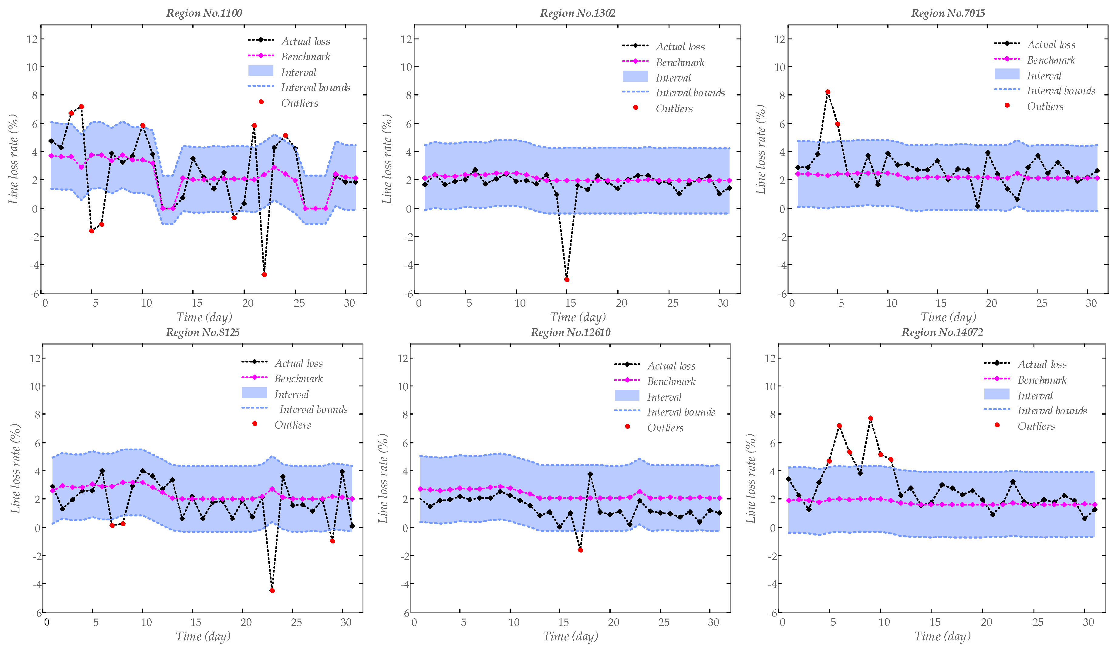
  • The line loss rate data possess few daily regularity and show high fluctuation. From Figure 1, the curves of line loss rates in different regions change greatly over the days, where historical line loss rates can be hardly used to estimate the further values. Thus, it is vital in this study to select influencing factors of line loss rate.
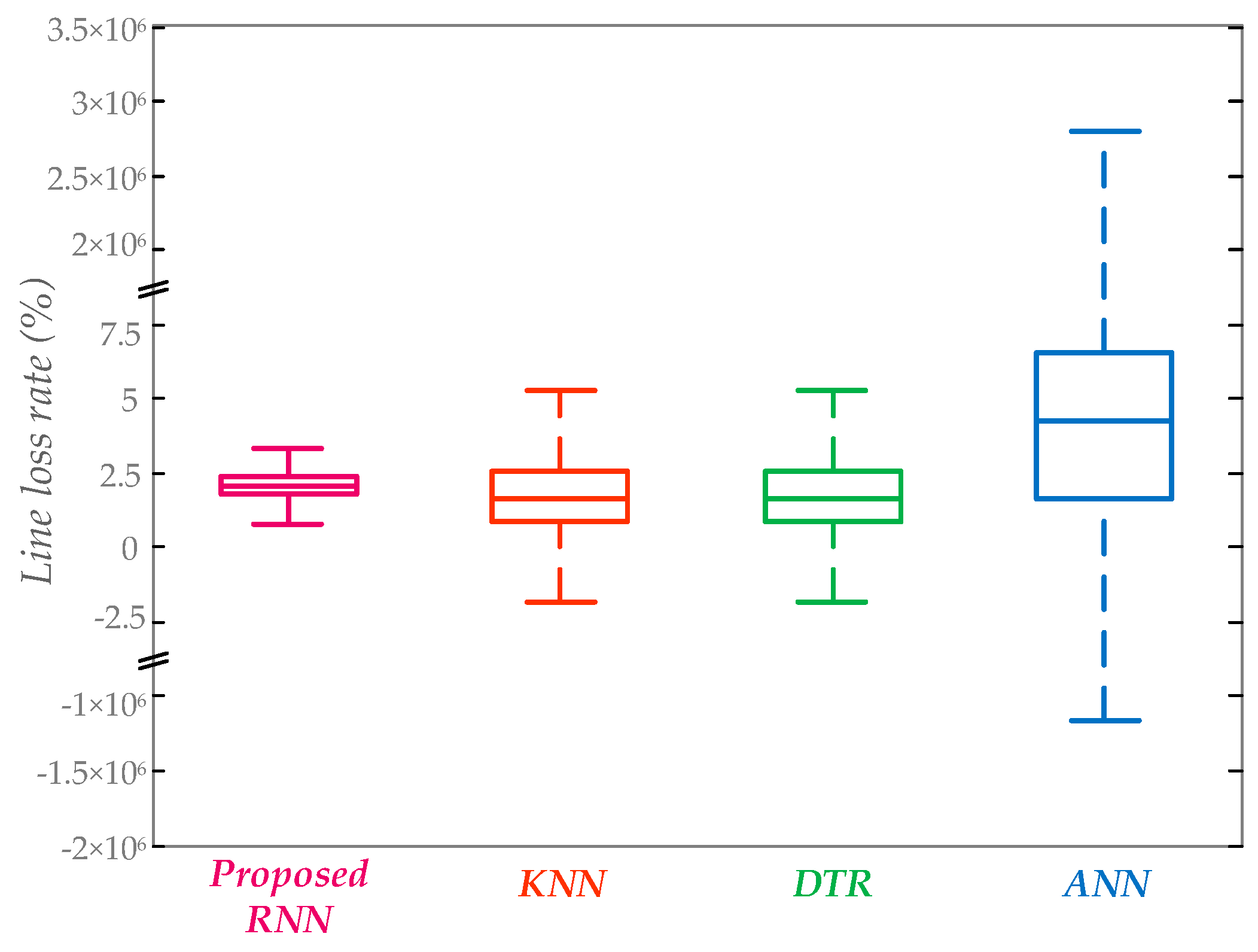
  • The deviations of outliers in the dataset are sometimes extremely away from normal values, indicating the low dependability of the acquisition and communication equipment. According to Table 1 and Figure 2, the lower and upper bounds of the original dataset in the box-plot are −1.57% and 5.22%, respectively, which is quite close to the project standard (−1% and 5%). However, the maximum and minimum of the collected line loss rates are 100% and −1.69 × 10⁶%, respectively; greatly different from the bounds. In this case, benchmarking line loss rates is still necessary nowadays in practicable applications.
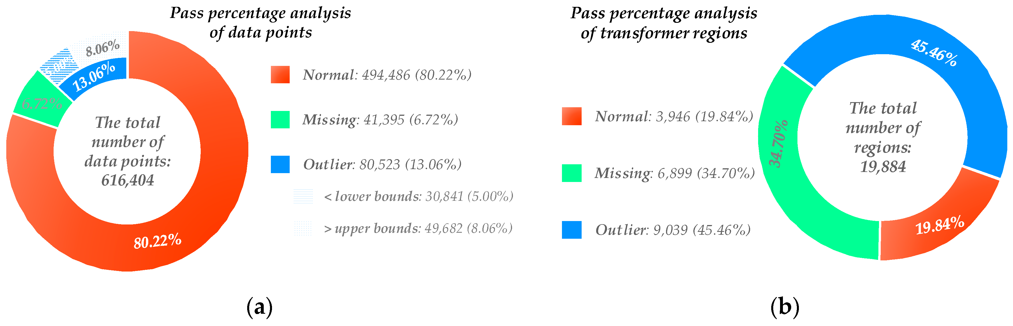
  • The quality of the dataset is poor to be used directly. As the component analysis of the dataset is presented in Figure 3, there are a large number of outliers and missing values, constituting 8.67% and 6.72% of the overall dataset. In this study, the spline interpolation method is utilized to fill the missing values. From Table 1 and Figure 2, the dataset after interpolation holds a similar distribution comparing to that of the original dataset. On the contrary, although the outliers can be eliminated directly based on la and ua, the distribution will change and it will be difficult to calculate an accurate reasonable intervals.

2.2.2. Influencing Factors of Line Loss Rate

Taking into account of both the possible influencing factors and the information recorded, a total of twelve factors are selected as inputs of the regression models, as shown in Table 2. Among those, the third and fourth factors are one-bit codes, while the others are numerical values.

2.3. Calculation of Benchmark Values and Reasonable Intervals

According to the data quality analysis, the original datasets contain a large quantile of outliers, which are far from the rational range, causing it much difficult to obtain an accurate result. Therefore, the task of this study is to utilize robust learning strategy and achieve a stable regression result away from outliers, as shown in Figure 4.
Commonly, there is a robust learning solution that one can set thresholds manually and delete outliers from the dataset according to those thresholds, where the rest of the dataset can be applied to train a machine learning model. However, it still remains a problem how to decide precise thresholds. Besides, computed bounds of the reasonable interval from the learning model may be close to the manual thresholds, which breaks the distribution of the original dataset and makes it meaningless to train a probabilistic learning model. In this case, the calculation method based on RNN is proposed, as shown in Figure 5, which consists of the following steps:
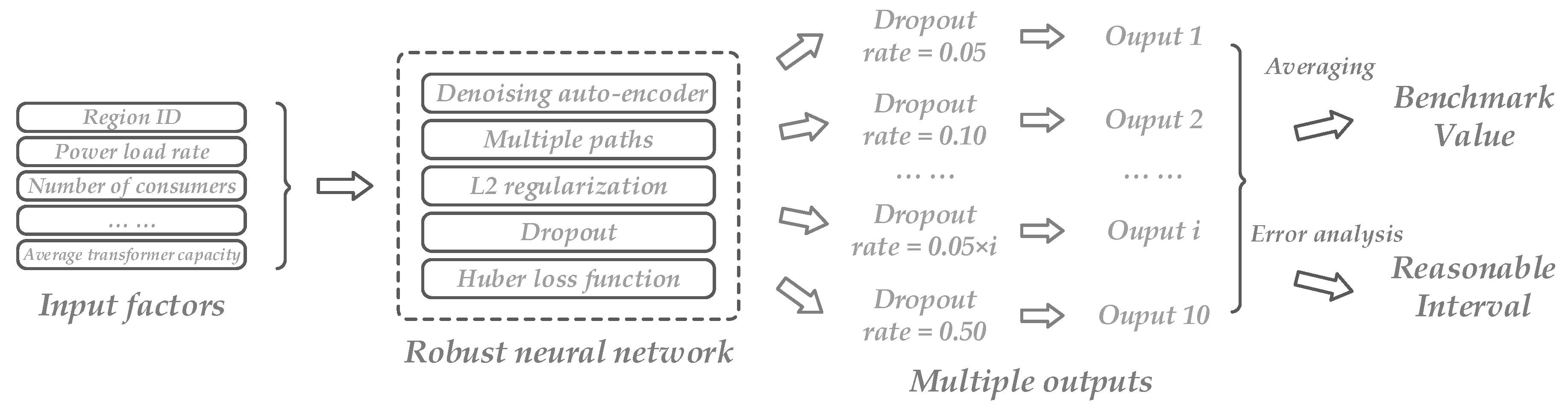
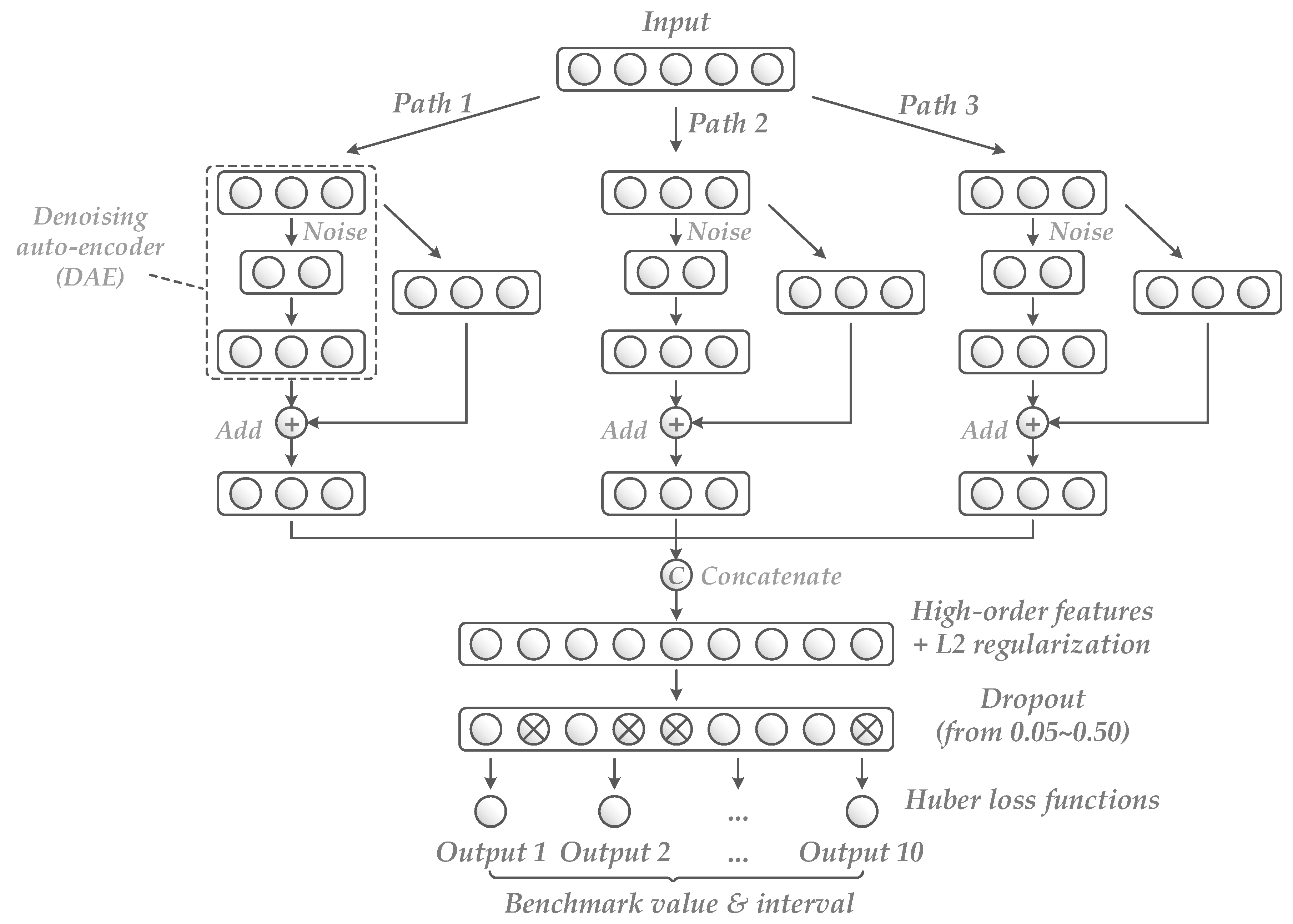
  • Build a RNN. In order to fully expand its robustness, DAE, multi-path architecture, L2 regularization, dropout layer and Huber loss function are applied. It is noted that a RNN possesses ten output nodes, where each node is connected to one layer with a dissimilar dropout rate (from 0.05 to 0.50).
  • Calculate an average value according to the ten different outputs, which is the final benchmark value of line loss rate, as:
    y ˜ i = 1 10 n = 1 10 y i n ,
    where y ˜ i is the ith benchmark value, and y i n is the nth output of the ith line loss rate.
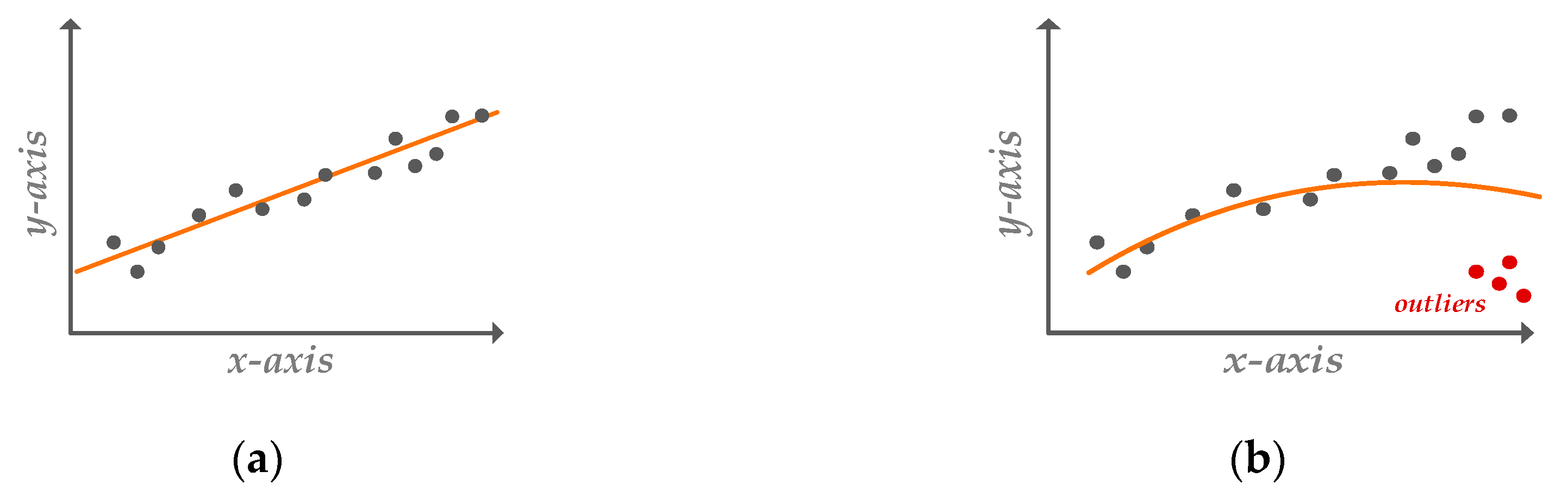
  • Operate error analysis to acquire a reasonable interval. Not only the absolute error between the benchmark value and the actual line loss rates is computed, the variance of different outputs is calculated as well. According to the interval result, data points that are not involved between the bounds of the interval are considered as outliers. The operation can be described under the following equations:
    e 1 = 1 n s i = 1 n s ( y ˜ i y i ) 2 ,
    e 2 = 1 10 1 i = 1 10 ( y ˜ i y i n ) 2 ,
    { l i = y ˜ i e 1 e 2 u i = y ˜ i + e 1 + e 2 ,
    where e1 and e2 are the results of error analysis. e1 is a constant and e2 changes according to the number i. ns is the number of training samples; y i is the ith actual line loss rate; li and ui are the lower and upper bounds of the reasonable interval, respectively. Furthermore, as outliers exist in the actual line loss rate values, which may influence the result of e1, a two-tailed test is utilized to eliminate the possibly abnormal y i values that are smaller than 0.7 percentile and bigger than 99.3 percentile, as shown in Figure 6:

2.4. Robust Neural Network

As mentioned before, an RNN is used in this study for robust learning, whose architecture is provided in Figure 7. It is made up of three main paths which are combined by concatenation, where there is a DAE on each main path. The concatenated output nodes are placed in a same layer, which represent high-order features extracted from original inputs. For the further improvement of robustness, L2 regularization is utilized in this layer to limit the output values of those nodes. Then, ten dropout layers with different dropout rate are stacked after the high-order feature layer, where ten outputs can be obtained. The ten outputs are analyzed to calculate the benchmark value and reasonable interval, as introduced above in Section 2.3.

2.4.1. Denoising Auto-Encoder

The architecture of DAE is provided in Figure 8. It is a robust variant of auto-encoder, which possesses a noise layer before encoder [32], such as a normal (Gaussian) noise layer:
x i , n = x i + N ( 0 , σ 2 ) ,
where xi and xi,n are the ith input and the ith output of the noise layer, respectively. N (0,σ2) is a normal distribution with a mean value of 0 and a variance value of σ2. In this study, σ is set to be 0.05 when the inputs are normalized into [0, 1].
Besides, the encoder and decoder layers in DAE are both made up of conventional fully-connected (FC) layers, whose equation can be expressed as:
y i l = w i j x j l 1 + b j ,
where y i l and x j l 1 are the ith output and the jth input of the lth layer, respectively; wij and bj are the weight and bias of the FC layer that connect the jth input and the ith output. For the encoder layer, the number of outputs is smaller than that of inputs, i.e., i < j; and the number of outputs in the decoder layer is equal to that of the original inputs. Hence, after the computation of DAE, the dimension and size of inputs remain unchanged, whereas the robustness of features increases as they can resist a certain degree of noise interference.

2.4.2. Multiple Paths Combined by Addition and Concatenation

There are altogether three main paths in RNN, which have similar layers and whose outputs are combined under a concatenation operation:
{ y c = C [ f k ( x , { w k n w , b k n b } ) ] y k , m p = f k ( x , { w k n w , b k n b } ) ,   k = 1 , 2 , 3 ,
where C(·) is the concatenation operation, which combines output nodes from different layers into an entire layer; yc and yk,mp are the output vector of the concatenation and the output vector of the kth main path, respectively; f k ( x , { w k n w , b k n b } ) is the computation result of the kth main path; x denotes the input vector of RNN; w k n w and b k n b are the weight matrixes and bias vectors of the kth path, respectively; nw and nb are the numbers of weights and biases, respectively.
Furthermore, a main path is formed by two sub-paths, i.e., a DAE sub-path and a FC layer sub-path. The outputs of the two sub-paths are added as the output of a main path, as follows:
y k , m p = f k ( x , { w k n w , b k n b } ) = g k ( x , { w k n w 1 , b k n b 1 } ) + ( w k s p x + b k s p )
where gk(·) represents the computation of DAE on the kth main path; w k s p and b k s p are the weight matrix and bias vector of the FC layer sub-path on the kth main path, respectively.

2.4.3. Dropout

Dropout is a special kind of layer, which is efficient to prevent over-fitting [33]. The procedure of dropout can be summarized into two steps, i.e., the training step and application step. For a conventional FC layer as expressed in Equation (12), there are j input nodes. In the training step, the input nodes will be abandoned under a probability p (0 < p < 1), where those abandoned nodes cannot be connected to outputs [34], as shown in Figure 9. After training, all the input nodes are operating in the application step, whereas the weight values are multiplied by the probability p, which can be described as:
y i l = p w i j x j l 1 + b j ,
where p is the probability, called dropout rate. It is a hyper-parameter and is set from 0.05 to 0.50, with a step of 0.05, in order to obtain ten different outputs in this study.

2.4.4. Huber Loss Function

The training process of neural network is to set a loss function and utilize back-propagation (BP) gradient descent algorithm to update the parameters layer by layer. One of the most common-used function is mean squared error (MSE):
MSE = 1 n s i = 1 n s ( y i y i ) 2 ,
where ns is the number of training samples; y i and y i are the ith predicted and the ith actual outputs, respectively. Besides, mean absolute error (MAE) is another conventional function, which can be defined as follows:
MAE = 1 n s i = 1 n s | y i y i | ,
where MSE and MAE can be also called L1 loss and L2 loss, as linear term and quadratic term are used in the MSE and MAE, respectively.
Comparing MSE and MAE, MSE holds a smoother derivative function, which can benefit the calculation of gradient descent algorithm, whereas a small difference in MAE may cause a huge change in parameter updating. On the contrary, MAE demonstrates a better capability than MSE when fighting against outliers [35]. In this case, a Huber loss function is applied in this study that combines the merits of both MSE and MAE [36], as shown in Figure 10:
Huber = 1 n s i = 1 n s { 1 2 ( y i y i ) 2 , | y i y i | δ δ | y i y i | 1 2 δ 2 , | y i y i | > δ ,
where δ is a hyper-parameter that needs to be set manually. It is set to be 10% in this study.

2.4.5. L2 Regularization

L2 regularization in this study is aimed to set a penalty term for the nodes that hold large activation outputs, in order to prevent over-fitting and increase robustness of the neural network. The regularization works during the training phase, where a two-norm penalty term is added to the training loss function [37], which can be expressed as follows:
L = λ y c 2 + Huber = λ y c 2 + 1 n s i = 1 n s { 1 2 ( y i y i ) 2 , | y i y i | δ δ | y i y i | 1 2 δ 2 , | y i y i | > δ
where L represents the final loss function for model training; and λ is a hyper-parameter of the penalty term, which is set to be 0.001 in this study.

3. Results and Discussion

The architecture and hyper-parameters of the proposed RNN are presented in Table 3. Moreover, considering the fact that there are a large number of training samples, k-nearest neighbors (KNN), decision tree regression (DTR) and single-hidden-layer artificial neural network (ANN) are established for comparisons, which hold relatively high training efficiency on big datasets. The training of the deep RNN model is conducted based on a personal computer with NVIDIA GTX 1080 GPU using Python 3.5 and Tensorflow 1.4. The calculation results and discussions are provided in detail as follows. It should be noted that all the hyper-parameters and training configurations of RNN, along with the hyper-parameters mentioned in Section 2.4 (i.e., σ, δ and λ), are chosen via gird search with three-fold cross-validation based on the overall training dataset. The searching spaces and final results of those parameters are listed in Table 4.

3.1. Calculation Results

In the case study, six regions from testing samples are chosen randomly as examples for exhibition, which are shown in Figure 11. Their region IDs are 1100, 1302, 7015, 8125, 12,610 and 14,072, respectively. From the results, the bounds of reasonable intervals can adjust adaptively according to multiple input factors, especially in Region No. 1100 and Region No. 8125. Some outliers that are far away from benchmarks are efficiently picked out, although those outliers may stay between −1% and 5%. Hence, the results of reasonable intervals are better than a fixed interval between −1% and 5%. Besides, the benchmark values show less fluctuation the actual line loss rate values, indicating a high reliability to estimate daily line loss rates. Rather than a mean value or a median value calculated from the original dataset, benchmark values are able to adaptively reflect the daily operating conditions in transformer regions according to the changes of relevant factors.
Based on the proposed RNN, the pass percentage results of line loss rates can be analyzed, which are shown in Figure 12. For the data point analysis of line loss rates, the number of outliers are more than that in Figure 3, as the proposed method is able to precisely identify those outliers that are greatly different from the benchmark values. Furthermore, although the percentages of missing values and outliers are not relatively big in all data points, which are 6.72% and 13.06%, respectively, the regions that possess no missing and abnormal values within a month only occupy 19.84% of the whole dataset in the study, indicating a low reliability of the current acquisition equipment.

3.2. Comparsions and Disscussion

In order to evaluate the performance of the proposed method, including robustness and accuracy, comparison studies are conducted in this section. The hyper-parameters of the established KNN, DTR and ANN are provided in Table 5. The comparison results are presented and discussed in detail as follows.

3.2.1. The Robustness of the Proposed Method

In order to evaluate the robustness of the proposed method, the distributions of the calculated benchmark values based on different testing models are analyzed, as shown in Figure 13. The detailed values of the distribution indictors are presented in Table 6. From the results, the testing ANN model shows the worst performance and is totally unable to calculate a valid benchmark value. The maximum and minimum values from the ANN are 4.49 × 10⁶% and −8.26 × 10⁷%, respectively, which can hardly be applied as benchmarks. KNN and DTR obtain similar results according to the distributions. They both utilize massive training samples that are close to the situation of an unknown testing region to decide new benchmark values. Thus, they are able to receive a better robustness than ANN in the study and are practicable at most of the testing regions. However, the minimum benchmark of the two models is −8.13 × 10⁴%, which is still not a reasonable value. Furthermore, the proposed RNN achieve the best result among all the four testing models, where the calculated benchmark values are within a reasonable range. The standard deviation of the benchmark values calculated by RNN is only 0.80%, indicating a stable and robust result obtained via the proposed method.

3.2.2. Accuracy Analysis

Besides the performance of robustness, accuracy is another important criterion in the study. As a result, three loss indicators are utilized to compare the four testing models, i.e., MAE, MSE and Huber loss, as their equations are discussed in Section 2.4.4. The outliers in the testing samples are eliminated before loss calculation using the two-tailed test, which is introduced above in Figure 6. The comparison result is shown in Table 7. According to the result, ANN performs the worst as its three loss indicators are much more than those of other models. Hence, the testing ANN is inapplicable when directly trained on samples with extreme outliers. Besides, although KNN and DTR show similar robustness, their accuracy indicators are quite different. KNN obtains the best MAE indicator, whereas the MSE value of KNN is bigger than that of the proposed RNN, due to the small number of outliers calculated by KNN. Comparing those indicators comprehensively, the proposed RNN shows the highest performance, as it achieves the best MSE and Huber loss indictors with a small MAE value as well.

4. Conclusions

Daily line loss rate is a critical indictor for power-supply corporations as it greatly affects their profits. In order to better manage the level of line losses and provide guidance for the construction and operation of low-voltage transformer regions, it is concerned with developing an efficient method to compute benchmark values for daily line loss rates. Based on the benchmarks, reasonable intervals of the daily line loss rates can be further obtained, which are able to help discover abnormal line loss rate values, as well to help operators to check and confirm those irregular operating conditions. However, the number of studies is limited that research on calculating benchmark values of daily line loss rates and eliminating outlier from collected line loss rate data. As a result, a regression calculation method based on RNN is proposed in this study. It consists of DAE, three main paths, dropout layers, Huber loss function, L2 regularization and ten outputs. The benchmarks are calculated according to the mean values of the ten outputs. After error analysis, reasonable intervals can be obtained to detect outliers of original line loss rate samples.
From the case study and comparison results, conventional ANN model fails to calculate results of benchmarks, as it cannot deal with outliers. KNN, DTR and the proposed RNN are proved applicable in the case study, where the proposed RNN outperforms the other two models. It shows both high accuracy and robustness among all the testing models. Furthermore, according to the final result obtained from the proposed RNN, there are about 13% outliers in the overall data points. The percentage of regions only occupy about 20% that hold no missing and abnormal values of line loss rates within a month, indicating a low dependability of the acquisition equipment. Therefore, a reliable monitoring and management system for line loss data is still necessary nowadays in power grid.

Author Contributions

Writing original draft preparation, W.W. and L.C.; reviewing and editing, Y.Z., B.X. and H.Z.; supervision, G.X. and X.L.

Funding

This research is supported by Science and Technology Project of Jiangsu Frontier Electric Technology Corporation, called “Research on key techniques of line loss benchmark value modeling in low-voltage transformer area by data-driven model” (project ID. 0FW-18553-WF).

Conflicts of Interest

The authors declare no conflict of interest.

References

  1. Chen, B.J.; Xiang, K.L.; Yang, L.; Su, Q.M.; Huang, D.S.; Huang, T. Theoretical Line Loss Calculation of Distribution Network Based on the Integrated electricity and line loss management system. In Proceedings of the China International Conference on Electricity, Tianjing, China, 17–19 September 2018; pp. 2531–2535. [Google Scholar]
  2. Yang, F.; Liu, J.; Lu, B.B. Design and Application of Integrated Distribution Network Line Loss Analysis System. In Proceedings of the 2016 China International Conference on Electricity Distribution (CICED), Xi’an, China, 10–13 August 2016. [Google Scholar]
  3. Hu, J.H.; Fu, X.F.; Liao, T.M.; Chen, X.; Ji, K.H.; Sheng, H.; Zhao, W.B. Low Voltage Distribution Network Line Loss Calculation Based on The Theory of Three-phase Unbalanced Load. In Proceedings of the 3rd International Conference on Intelligent Energy and Power Systems (IEPS 2017), Hangzhou, China, 10 October 2017; pp. 65–71. [Google Scholar] [CrossRef] [Green Version]
  4. Campos, G.O.; Zimek, A.; Sander, J.; Campello, R.J.G.B.; Micenkova, B.; Schubert, E.; Assent, I.; Houle, M.E. On the evaluation of unsupervised outlier detection: Measures, datasets, and an empirical study. Data Min. Knowl. Disc. 2016, 30, 891–927. [Google Scholar] [CrossRef]
  5. Paulheim, H.; Meusel, R. A decomposition of the outlier detection problem into a set of supervised learning problems. Mach. Learn. 2015, 100, 509–531. [Google Scholar] [CrossRef]
  6. Daneshpazhouh, A.; Sami, A. Entropy-based outlier detection using semi-supervised approach with few positive examples. Pattern Recogn. Lett. 2014, 49, 77–84. [Google Scholar] [CrossRef]
  7. Bhattacharya, G.; Ghosh, K.; Chowdhury, A.S. Outlier detection using neighborhood rank difference. Pattern Recogn. Lett. 2015, 60–61, 24–31. [Google Scholar] [CrossRef]
  8. Domingues, R.; Filippone, M.; Michiardi, P.; Zouaoui, J. A comparative evaluation of outlier detection algorithms: Experiments and analyses. Pattern Recogn. 2018, 74, 406–421. [Google Scholar] [CrossRef]
  9. Dovoedo, Y.H.; Chakraborti, S. Boxplot-Based Outlier Detection for the Location-Scale Family. Commun. Stat.-Simul. Comput. 2015, 44, 1492–1513. [Google Scholar] [CrossRef]
  10. Pranatha, M.D.A.; Sudarma, M.; Pramaita, N.; Widyantara, I.M.O. Filtering Outlier Data Using Box Whisker Plot Method For Fuzzy Time Series Rainfall Forecasting. In Proceedings of the 2018 4th International Conference on Wireless and Telematics (ICWT), Nusa Dua, Indonesia, 12–13 July 2018. [Google Scholar]
  11. Campello, R.J.G.B.; Moulavi, D.; Zimek, A.; Sander, J. Hierarchical Density Estimates for Data Clustering, Visualization, and Outlier Detection. ACM Trans. Knowl. Discov. Data 2015, 10, 5. [Google Scholar] [CrossRef]
  12. Huang, J.L.; Zhu, Q.S.; Yang, L.J.; Cheng, D.D.; Wu, Q.W. A novel outlier cluster detection algorithm without top-n parameter. Knowl.-Based Syst. 2017, 121, 32–40. [Google Scholar] [CrossRef]
  13. Jiang, F.; Liu, G.Z.; Du, J.W.; Sui, Y.F. Initialization of K-modes clustering using outlier detection techniques. Inf. Sci. 2016, 332, 167–183. [Google Scholar] [CrossRef]
  14. Todeschini, R.; Ballabio, D.; Consonni, V.; Sahigara, F.; Filzmoser, P. Locally centred Mahalanobis distance: A new distance measure with salient features towards outlier detection. Anal. Chim. Acta 2013, 787, 1–9. [Google Scholar] [CrossRef]
  15. Jobe, J.M.; Pokojovy, M. A Cluster-Based Outlier Detection Scheme for Multivariate Data. J. Am. Stat. Assoc. 2015, 110, 1543–1551. [Google Scholar] [CrossRef]
  16. An, W.J.; Liang, M.G.; Liu, H. An improved one-class support vector machine classifier for outlier detection. Proc. Inst. Mech. Eng. C J. Mech. 2015, 229, 580–588. [Google Scholar] [CrossRef]
  17. Chen, G.J.; Zhang, X.Y.; Wang, Z.J.; Li, F.L. Robust support vector data description for outlier detection with noise or uncertain data. Knowl.-Based Syst. 2015, 90, 129–137. [Google Scholar] [CrossRef]
  18. Zou, C.L.; Tseng, S.T.; Wang, Z.J. Outlier detection in general profiles using penalized regression method. IIE Trans. 2014, 46, 106–117. [Google Scholar] [CrossRef]
  19. Peng, J.T.; Peng, S.L.; Hu, Y. Partial least squares and random sample consensus in outlier detection. Anal. Chim. Acta 2012, 719, 24–29. [Google Scholar] [CrossRef]
  20. Ni, L.; Yao, L.; Wang, Z.; Zhang, J.; Yuan, J.; Zhou, Y. A Review of Line Loss Analysis of the Low-Voltage Distribution System. In Proceedings of the 2019 IEEE 3rd International Conference on Circuits, Systems and Devices (ICCSD), Chengdu, China, 23–25 August 2019; pp. 111–114. [Google Scholar]
  21. Yuan, X.; Tao, Y. Calculation method of distribution network limit line loss rate based on fuzzy clustering. IOP Conf. Ser. Earth Environ. Sci. 2019, 354, 012029. [Google Scholar] [CrossRef]
  22. Bo, X.; Liming, W.; Yong, Z.; Shubo, L.; Xinran, L.; Jinran, W.; Ling, L.; Guoqiang, S. Research of Typical Line Loss Rate in Transformer District Based on Data-Driven Method. In Proceedings of the 2019 IEEE Innovative Smart Grid Technologies-Asia (ISGT Asia), Chengdu, China, 21–24 May 2019; pp. 786–791. [Google Scholar]
  23. Yao, M.T.; Zhu, Y.; Li, J.J.; Wei, H.; He, P.H. Research on Predicting Line Loss Rate in Low Voltage Distribution Network Based on Gradient Boosting Decision Tree. Energies 2019, 12, 2522. [Google Scholar] [CrossRef] [Green Version]
  24. Zhang, S.; Dong, X.; Xing, Y.; Wang, Y. Analysis of Influencing Factors of Transmission Line Loss Based on GBDT Algorithm. In Proceedings of the 2019 International Conference on Communications, Information System and Computer Engineering (CISCE), Haikou, China, 5–7 July 2019; pp. 179–182. [Google Scholar]
  25. Wang, S.X.; Dong, P.F.; Tian, Y.J. A Novel Method of Statistical Line Loss Estimation for Distribution Feeders Based on Feeder Cluster and Modified XGBoost. Energies 2017, 10, 2067. [Google Scholar] [CrossRef] [Green Version]
  26. Radovanovic, M.; Nanopoulos, A.; Ivanovic, M. Reverse Nearest Neighbors in Unsupervised Distance-Based Outlier Detection. IEEE Trans. Knowl. Data Eng. 2015, 27, 1369–1382. [Google Scholar] [CrossRef]
  27. Yosipof, A.; Senderowitz, H. k-Nearest Neighbors Optimization-Based Outlier Removal. J. Comput. Chem. 2015, 36, 493–506. [Google Scholar] [CrossRef]
  28. Wang, X.C.; Wang, X.L.; Ma, Y.Q.; Wilkes, D.M. A fast MST-inspired kNN-based outlier detection method. Inf. Syst. 2015, 48, 89–112. [Google Scholar] [CrossRef]
  29. Yang, J.H.; Deng, T.Q.; Sui, R. An Adaptive Weighted One-Class SVM for Robust Outlier Detection. Lect. Notes Electr. Eng. 2016, 359, 475–484. [Google Scholar] [CrossRef]
  30. Feng, N.; Jianming, Y. Low-Voltage Distribution Network Theoretical Line Loss Calculation System Based on Dynamic Unbalance in Three Phrases. In Proceedings of the 2010 International Conference on Electrical and Control Engineering, Wuhan, China, 25–27 June 2010; pp. 5313–5316. [Google Scholar]
  31. Hubert, M.; Vandervieren, E. An adjusted boxplot for skewed distributions. Comput. Stat. Data Anal. 2008, 52, 5186–5201. [Google Scholar] [CrossRef]
  32. Lamb, A.; Binas, J.; Goyal, A.; Serdyuk, D.; Subramanian, S.; Mitliagkas, I.; Bengio, Y. Fortified Networks: Improving the Robustness of Deep Networks by Modeling the Manifold of Hidden Representations. arXiv 2018, arXiv:1804.02485. [Google Scholar]
  33. Srivastava, N.; Hinton, G.; Krizhevsky, A.; Sutskever, I.; Salakhutdinov, R. Dropout: A Simple Way to Prevent Neural Networks from Overfitting. J. Mach. Learn. Res. 2014, 15, 1929–1958. [Google Scholar]
  34. Cheng, L.L.; Zang, H.X.; Ding, T.; Sun, R.; Wang, M.M.; Wei, Z.N.; Sun, G.Q. Ensemble Recurrent Neural Network Based Probabilistic Wind Speed Forecasting Approach. Energies 2018, 11, 1958. [Google Scholar] [CrossRef] [Green Version]
  35. Friedman, J.H. Greedy function approximation: A gradient boosting machine. Ann. Stat. 2001, 29, 1189–1232. [Google Scholar] [CrossRef]
  36. Esmaeili, A.; Marvasti, F. A Novel Approach to Quantized Matrix Completion Using Huber Loss Measure. IEEE Signal Proc. Lett. 2019, 26, 337–341. [Google Scholar] [CrossRef]
  37. Shah, P.; Khankhoje, U.K.; Moghaddam, M. Inverse Scattering Using a Joint L1-L2 Norm-Based Regularization. IEEE Trans. Antennas Propag. 2016, 64, 1373–1384. [Google Scholar] [CrossRef]
Figure 1. Examples of daily line loss rates in July 2018 from different regions in Wuxi, Jiangsu Province, China.
Applsci 09 05565 g001
Figure 2. The distribution box-plots of original dataset and the dataset after interpolation operation.
Applsci 09 05565 g002
Figure 3. The component result of data quality analysis (84.61% normal values, 8.67% outliers and 6.72% missing values).
Applsci 09 05565 g003
Figure 4. Conventional learning methods may be easily affected by outliers. (a) Common condition; (b) affected by outliers.
Applsci 09 05565 g004
Figure 5. The flowchart of the proposed method in this study for calculating benchmark values and reasonable intervals based on robust neural network (RNN).
Applsci 09 05565 g005
Figure 6. A two-tailed test to eliminate possibly abnormal line loss rate values.
Applsci 09 05565 g006
Figure 7. The architecture of the proposed robust neural network (RNN).
Applsci 09 05565 g007
Figure 8. The architecture of denoising auto-encoder (DAE).
Applsci 09 05565 g008
Figure 9. The principle of dropout during the training step.
Applsci 09 05565 g009
Figure 10. The principle of Huber loss function.
Applsci 09 05565 g010
Figure 11. The results of benchmark values and reasonable intervals in six testing regions.
Applsci 09 05565 g011
Figure 12. Pass percentage analysis of the line loss rates based on robust neural network (RNN). (a) Analysis of data points; (b) analysis of transformer regions.
Applsci 09 05565 g012
Figure 13. The distributions of the calculated benchmark values based on different testing models.
Applsci 09 05565 g013
Table 1. The data quality analysis based on the overall line loss rate dataset.
IndicatorOriginal DatasetOriginal Dataset
(Without Outliers)
Dataset after Interpolation
mean (%)−5.161.78−10.96
std (%)2.47 × 1031.163.19 × 103
min (%)−1.69 × 10⁶−1.57−1.69 × 10⁶
max (%)1005.22100
la (%)−1.57−1.10−1.50
ua (%)5.224.575.26
q1 (%)1.021.021.03
q2 (%)1.741.671.76
q3 (%)2.702.442.72
Table 2. Influencing factors of line loss rate utilized in this study.
No.FactorRemarks
1Date-
2Capacity of the transformer-
3Type of the transformerPublic transformer (=0); special transformer (=1)
4Type of the gird that the region belongs toCity grid (=0); country gird (=1)
5Monthly line loss rateThree inputs, including the last three months
6Daily load rateDaily load rate = daily power supply/(transformer capacity × 24)
7Daily maximum load rate-
8Daily average power factor-
9Number of customers-
10Average transformer capacity per customerAverage capacity = transformer capacity/number of customers
11Rate of residential capacityRate = residential capacity/transformer capacity
12Power supply duration-
Table 3. The architecture and hyper-parameters of the proposed robust neural network (RNN).
PathLayerHyper-Parameter
DAE sub-path (1~3)FC layer 0Node number: 64
Activation: ReLU (Rectified Linear Unit)
DAE sub-path (1~3)Noise layerStandard deviation: 0.05
DAE sub-path (1~3)FC layer 1 (encoder)Node number: 8
Activation: ReLU
DAE sub-path (1~3)FC layer 2 (decoder)Node number: 64
Fully connected (FC) sub-path (1~3)FC layer 3Node number: 64
Main path (1~3)Add layerInputs: FC layer 2 and FC layer 3
-Concatenate layerInputs: Add layers
Node number: 192
Activation: ReLU
Activity regularization: L2, λ = 1 × 10⁻³
-Dropout layer (1~10)Dropout rate: 0.05~0.50 (0.05 step)
-FC layer 4 (output 1~10)Node number: 1
Activation: ReLU
Table 4. The searching spaces of selected hyper-parameters in RNN.
Hyper-ParametersSearching SpaceResult
σ (standard error of noise in DAE)[0.00:0.05:0.50]0.05
δ (coefficient in Huber loss)[0.00:0.10:0.50]0.10
λ (penalty coefficient of L2)1 × 10[−4:1:0]1 × 10⁻³
Number of nodes in a sub-path{16, 32, 64, 128}64
Number of sub-paths[2:1:5]3
Training optimizer{Adadelta, Adam}Adam
Number of epochs[50:50:200]100
Batch size{64, 128, 256, 512, 1024, 2048}1024
Learning rate1 × 10[−5:1:0]1 × 10⁻⁴
Table 5. The hyper-parameters of the established k-nearest neighbors (KNN), decision tree regression (DTR) and artificial neural network (ANN).
ModelHyper-Parameter
KNNNumber of neighbors: 10
Method of weighting: based on distance
DTRMethod of splitter: choose the best spilt
ANNNode number in the hidden layer: 64
Activation: logistic
Table 6. The robustness analysis results of different testing models.
IndicatorProposed RNNKNNDTRANN
mean (%)2.031.03−4.81−5.83 × 10⁶
std (%)0.80185.69194.781.87 × 107
min (%)0.00−8.13 × 10⁴−8.13 × 10⁴−8.26 × 10⁷
max (%)33.61100.00100.004.49 × 106
la (%)0.81−1.80−1.80−1.17 × 10⁶
ua (%)3.365.255.242.80 × 106
q1 (%)1.760.840.843.23 × 105
q2 (%)2.091.651.658.47 × 105
q3 (%)2.402.602.601.32 × 106
Table 7. The accuracy analysis results of different testing models.
IndicatorProposed RNNKNNDTRANN
Mean absolute error (MAE, %)1.460.705.017.26 × 106
Mean squared error (MSE, %2)13.70574.583.90 × 1033.54 × 1014
Huber loss4.445.9048.197.26 × 107

