Modelling Timbral Hardness


Institute of Sound Recording, Department of Music and Media, University of Surrey, Guildford, Surrey GU2 7XH, UK
*
Author to whom correspondence should be addressed.
Appl. Sci. 2019, 9(3), 466; https://0-doi-org.brum.beds.ac.uk/10.3390/app9030466
Submission received: 10 December 2018
/
Revised: 15 January 2019
/
Accepted: 24 January 2019
/
Published: 30 January 2019
(This article belongs to the Special Issue Psychoacoustic Engineering and Applications)
Abstract
:Featured Application
The model of timbral hardness described in this study is expected to be used for the searching and filtering of sound effects.
Abstract
Hardness is the most commonly searched timbral attribute within freesound.org, a commonly used online sound effect repository. A perceptual model of hardness was developed to enable the automatic generation of metadata to facilitate hardness-based filtering or sorting of search results. A training dataset was collected of 202 stimuli with 32 sound source types, and perceived hardness was assessed by a panel of listeners. A multilinear regression model was developed on six features: maximum bandwidth, attack centroid, midband level, percussive-to-harmonic ratio, onset strength, and log attack time. This model predicted the hardness of the training data with = 0.76. It predicted hardness within a new dataset with = 0.57, and predicted the rank order of individual sources perfectly, after accounting for the subjective variance of the ratings. Its performance exceeded that of human listeners.
1. Introduction
Many online sound effects repositories exist, such as freesound.org, freeSFX.co.uk, and zapsplat.com, where users can upload sounds to be hosted under a Creative Commons (CC) licence. The Audio Commons project is aimed at promoting the creative reuse of CC-licensed audio content. One method of encouraging reuse is to make it easier for users to search for desired sound effects.
Most online sound effect repositories employ some form of keyword searching—matching user search queries to titles and/or tags that uploaders have manually ascribed to the sounds. Therefore, the ability to find a desired sound effect is limited by the quality and quantity of the user-supplied metadata, which may be sparse or inconsistent. Some curated repositories also provide technical metadata, such as sample rate and bit depth, or musical descriptors, such as tempo or genre. The technical descriptors, whilst useful, describe the audio file format rather than the sonic content and many of the musical descriptors are not applicable to sound effects (e.g., a recording of a door slam has no tempo).
The freesound.org repository can additionally provide metadata calculated with the essentia toolbox [1]. However, most of these metadata are technical measurements, such as spectral flux, spectral kurtosis, or silence rate, which are unlikely to be meaningful to the non-acoustician. For such a user, timbral descriptors would be more readily understood and would provide more useful assistance in the search for a desired sound. Therefore, it would be beneficial if timbral metadata could be generated automatically, using perceptual models to tag audio files with their timbral characteristics.
1.1. Which Timbral Attribute?
Timbre is a multidimensional property of sound [2,3], and as such is comprised of multiple attributes, such as hardness, brightness, and roughness [4,5,6,7]. Many experiments have sought to identify the salient attributes of timbre for various source types and situations. One common method, for example, employs statistical dimensional reduction techniques, such as multi-dimensional scaling, to determine the number of attributes and then verbal and semantic analysis techniques to derive meaningful labels for them [8,9,10,11,12]. Similar methods have been employed in the investigation of environmental soundscape descriptors [11,13]. The contents of online sound effects repositories cover a vast range of source types and might ultimately be used in a very large number of applications. Therefore, to determine the timbral attributes that would be most useful in sound effects searches, a meta-analysis was conducted by Pearce et al. [14].
Pearce et al. collated a comprehensive list of timbral attributes from multiple research papers spanning multiple audio research disciplines [14]. They then used the search history of freesound.org to determine the frequency with which each of these attributes appeared in search queries. The most frequently used timbral search term was hardness. Therefore, a perceptual model able to predict the perceived hardness of a sound would allow automatic generation of metadata that would be particularly useful for augmenting sound effect searching.
1.2. Previous Models
Hardness has been identified as an important timbral attribute in studies relating to soundscapes [12], loudspeakers [8], musical acoustics [15], sound synthesis [16,17], spatial audio [18], and timbral semantics [19,20,21,22,23]. Some of these studies were conducted in languages other than English [20,21], indicating that the importance of hardness as a timbral descriptor is not English-specific.
Despite the apparent importance of the hardness attribute, there is little research into how it might be modelled. In research by Freed, listening tests were conducted where subjects were asked to rate the apparent physical hardness of a mallet used to strike a series of metal bars [5]. The research suggested four features appropriate for the prediction of hardness: the mean across time of the time-varying spectral centroid; the time weighted-average of the time-varying spectral centroid; the mean across time of the time-varying spectral level (log of the sum of the spectral energy for successive time frames); and the slope of the time-varying spectral level. A multilinear regression of these four features achieved good correlation to subjective results ( = 0.725). However, although human perception of a sound’s timbral hardness might often relate to perception of the physical hardness of the sound-making object, the applicability of this model to timbral hardness prediction is uncertain. Furthermore, its applicability to predicting the hardness of sounds produced by means other than physical impact is less certain still.
In the work of Czedik-Eysenberg et al. [6,7], a model of musical hardness was developed. Excerpts of contemporary music recordings were played to listeners who rated each for hardness on a seven-point scale. A linear regression model based on the level of percussive energy, the intensity of signal components between 2 kHz and 4 kHz, and the low centroid rate (percentage of analysis frames with a spectral centroid less than the average across the whole excerpt) predicted listener ratings with = 0.723. However, the study treated musical hardness as an element of genre (akin to musical ’heaviness’) rather than as a timbral attribute. Therefore, the applicability of the model to the prediction of the timbral hardness of non-musical sound effects is, again, far from certain.
Other research has been conducted on a morphing algorithm for softness, the antonym of hardness [24]. In this work, it was suggested that softness is related to the attack time of a signal. No model attempting to predict perceived softness was created, but features were discussed that may be useful in the modelling of perceived softness/hardness. Finally, although timbral and spatial aspects of sound can sometimes interact and/or overlap, Zacharov’s work on audio descriptors and spatial sound [18] found no evidence of any influence of spatial reproduction factors on timbral hardness.
1.3. Aims of the Current Study
Existing hardness models, discussed above, have been designed: (i) to predict mallet hardness or musical hardness, rather than timbral hardness; and (ii) for use only with a specific type of sound (percussive or musical). For the automated generation of hardness metadata to aid online sound effect repository searching, a model is needed that can predict timbral hardness for a wide range of sound sources. The research documented in this paper aimed to develop a model meeting this need such that, ultimately, repository search results might be generated, filtered or ordered according to timbral hardness. Section 2 describes the process of assembling and annotating a suitable corpus of sound effects. Section 3 details the implementation of methods for extracting features that may correlate with the perception of hardness. These extracted features are then used to develop a model of hardness in Section 4. The developed model is validated in Section 5, and its performance is discussed in Section 6.
Ethical approval for the study was granted by the University of Surrey Ethics Committee’s online self-assessment system (project id. 160708-160702-28785967, 12 January 2018). All subjects gave informed consent and all data were collected and stored anonymously.
2. Ratings of Hardness
To provide a dataset on which to base a model, listener ratings of hardness must be obtained for a suitable set of sounds. Since the developed model is intended to provide useful metadata for sound effect repositories, the set of sounds should (i) include those made by sources for which the option of searching by hardness is likely to be useful, (ii) be indicative of the types and qualities of sounds found on these repositories, and (iii) cover a wide range of perceived hardness.
2.1. Selecting Sound Source Types
Sound source types for which hardness metadata would be useful are likely to be those that are commonly searched for along with the terms hard or soft. One month’s search history from freesound.org, from April 2016, was analysed; this comprised 8,154,586 individual searches, grouped into 879,976 unique searches. For 2188 unique searches the terms hard or soft were included in the search query.
From inspection of these searches, it was clear that the terms hard and soft were often used in a non-timbral sense, e.g., ‘hardstyle’, ‘hardcore’, ‘airsoft’, etc. Three independent experts were asked to evaluate all the matching searches, marking those where the terms hard and soft were used in a non-timbral sense. Searches marked as such by two or more assessors were removed. The retained search queries were then manually grouped based on the specified source type, e.g., grouping searches for ‘hard kick’, ‘soft kick’, and ‘hard kick drum’. This left 273 unique source types. Of these, 36 were searched for on average at least once per day.
2.2. Acquisition of Stimuli
To ensure that all stimuli are indicative of the types and qualities of sound effects found in repositories, stimuli for the listening tests were acquired from freesound.org. For each of the 36 source types, a keyword search was performed using the freesound application programming interface (API), limiting the results to sound effects shorter than 20 s (a suitable maximum duration for listening test stimuli). Three searches were conducted for each source type: once for the source type in isolation (e.g., “snare”); once for the source type in combination with ‘hard’ (e.g., “hard snare”); and once for the source type in combination with ‘soft’ (e.g., “soft snare”).
From the results of each search, 50 unique random sound effects were downloaded, providing 150 stimuli per source type. All downloaded sounds were converted to two-channel wav files at 44.1 kHz sample rate. Any sound that, on audition, was found to be of a source type other than that specified was removed manually. Of the remaining sounds, for the source-type-only search the first 10 were retained; for the source-plus-‘hard’ the first five were retained; for the source-plus-‘soft’ the first five were retained. This left a total of 20 stimuli for each source type.
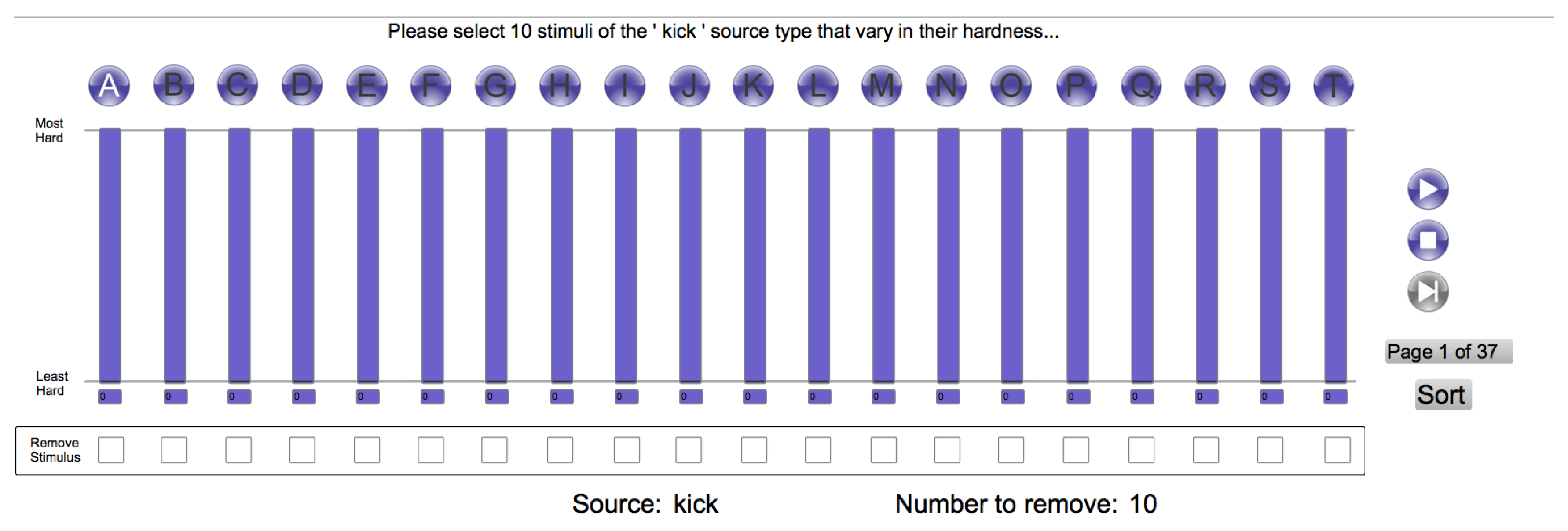
To ensure that the stimuli used in the listening test covered a wide range of perceived hardness, a small experiment was conducted using an independent expert listener. A multi-page user interface presented the 20 stimuli of a single source type on each test page (Figure 1). For each page, the listener was asked to (i) remove any stimuli they considered to not be of the source type specified; (ii) select the most and least hard stimuli, and (iii) select further stimuli, equally spaced between the most and least hard. The number of further stimuli requested was source-type-specific and was determined such that the total number of stimuli for each particular source type was: (i) between two and 10; and (ii) proportional to the average frequency with which searches for that source type had been made during the month for which freesound.org data were analysed. The selected 206 stimuli were then loudness normalised using the ffmpeg loudnorm function to LUFS [25].
For use as anchors in the listening test, the same independent expert then selected the two stimuli they considered to be the most and least hard stimuli from the full 206. Finally, they were asked to select six other stimuli of different source types to those selected for hidden anchors that were approximately evenly spaced between the two anchors on a scale of hardness. These were used in a test of inter-subject consistency, as described in Section 2.3.
2.3. Listening Test
Due to the large number of stimuli, the listening test was split into two test sessions. Before each test session, subjects were presented with a familiarisation interface comprising 20 stimuli on each page. Subjects were asked to listen to at least the first page, and then as many pages as required until they felt comfortable with the full range of hardness exhibited by the stimuli. The stimulus order was randomised between subjects, but the high and low anchor stimuli were always on the first page.
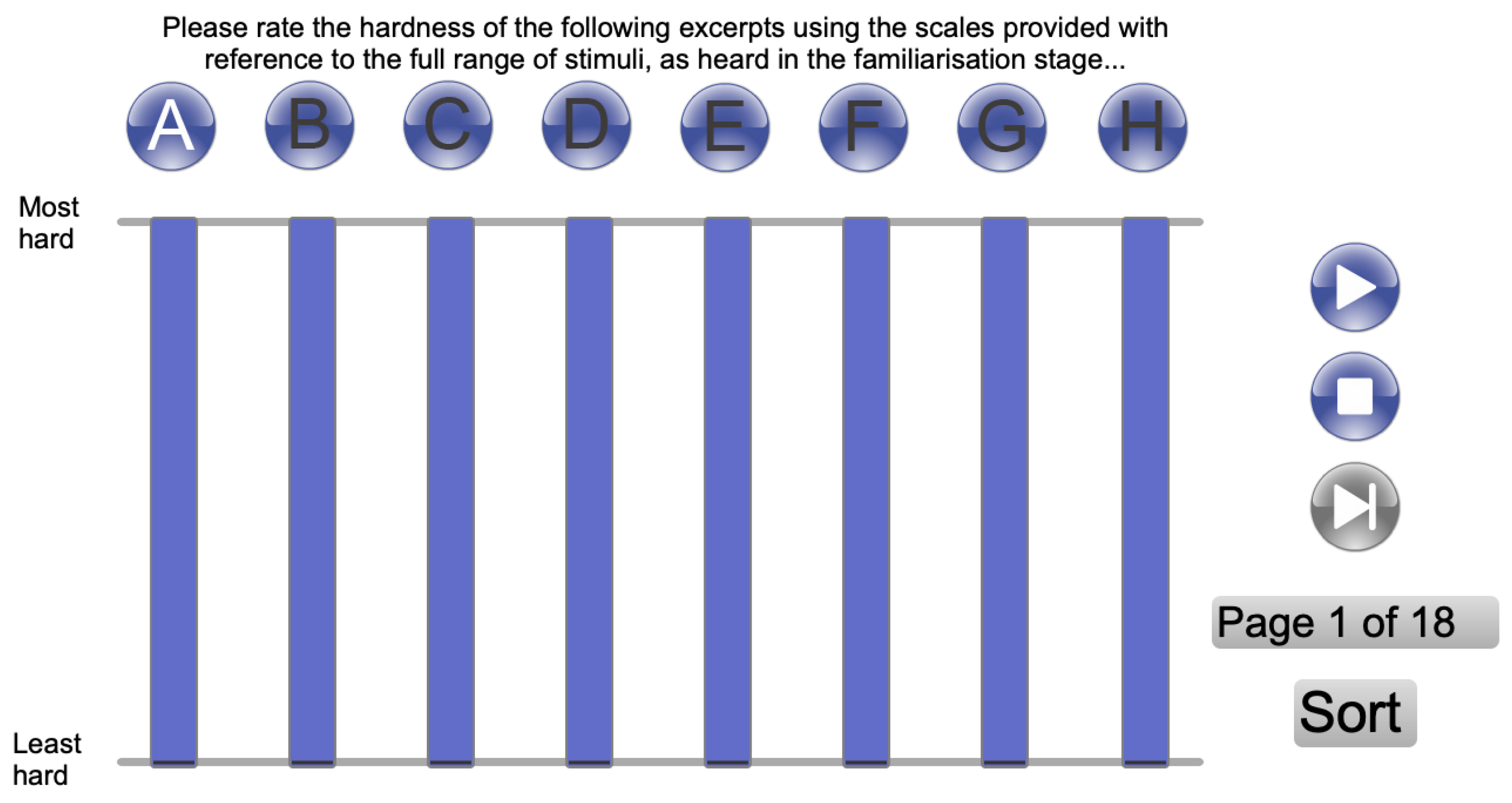
The listening test consisted of 18 pages per test session. On each page, eight stimuli were presented: the two hidden anchors and six randomly selected stimuli from the remaining 204 (with the exception of one test page per session that comprised the two hidden anchors and the six stimuli selected for assessing listener consistency). The test interface is shown in Figure 2. Subjects were asked to rate the perceived hardness of the eight stimuli on each page considering the full range of hardnesses encountered during the familiarisation. Subjects were able to audition each stimulus as many times as required and to sort the stimuli into ascending order according to their ratings.
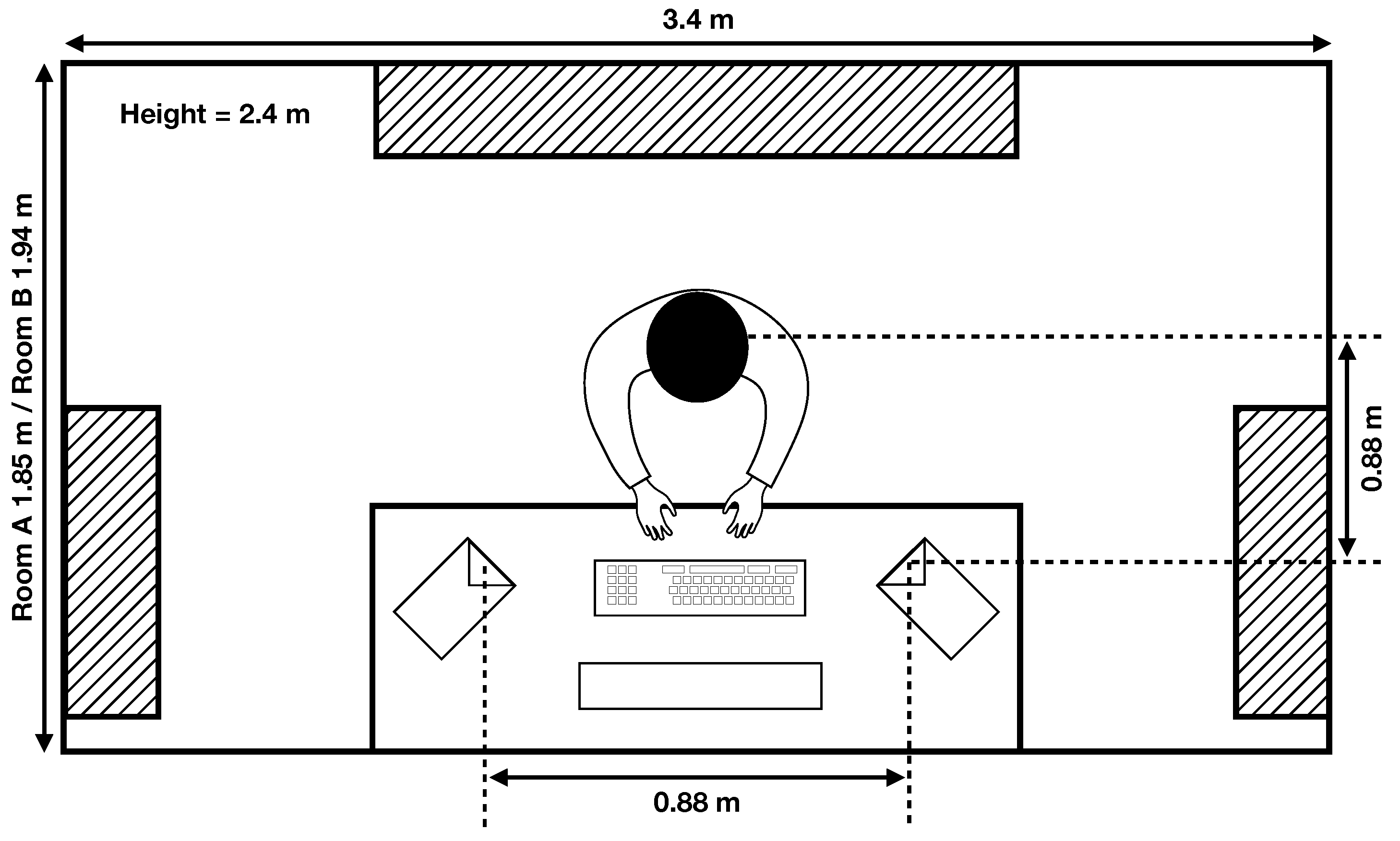
Listening tests were conducted in two acoustically treated edit suites at the University of Surrey, using Neumann KH 120 A loudspeakers. A plan view of the suites is provided in Figure 3. The replay system was adjusted so that pink noise at dBFS was reproduced at the listening position at 68 , a level found to be sufficiently loud to hear the nuances of the stimuli whilst being comfortable for a test session of approximately 25 min.
Seventeen listeners participated in the listening test (15 male, 2 female, mean age = 21.1 ± 1.1 years). All were undergraduate students in the Music and Sound Recording course at the University of Surrey; all self-reported normal hearing; all had participated in multiple listening tests previously; and all had passed a taught module in technical listening. It has been shown that in experiments such as those in the current study, results obtained from trained listeners reveal the same trends and rank orderings as those from untrained listeners but with less statistical noise. Thus, with trained listeners generalisability is maintained but statistical significance can be obtained with fewer trials [26,27].
2.4. Results
The performance of listeners was assessed by examining the inter-subject agreement, intra-subject consistency, and Tucker-1 correlation loadings [28,29]. From the Tucker-1 correlation loadings, subjects 4, 7, 9, 14, and 17 appeared to have different decision criteria when rating hardness, potentially leading to larger variance in the dataset. These subjects also performed worse than one standard deviation below the grand mean of the inter-subject agreement metric, and were therefore removed from subsequent analysis.
Results for the test pages used to test intra-subject consistency were removed prior to analysis to maintain balanced datasets, and the results were averaged across all subjects. These 206 mean ratings were used to develop a model of hardness.
3. Feature Extraction
To model the hardness ratings, features must be extracted that are thought to relate to the perception of hardness. All features were extracted using functions written in Python 2.7. Considering work such as that of Zacharov, discussed in Section 1.2, there was no reason to believe that spatial differences would contribute to perceived hardness [18]. As such, the stimuli were summed to mono before feature extraction. Whilst assessing the stimuli, several were identified as not suitable for feature extraction. Four stimuli were removed due to (i) inter-channel differences resulting in severe comb filtering when summing to mono; (ii) extremely poor signal-to-noise ratio; or (iii) the presence of additional background sounds that would be analysed by the feature extraction algorithms yet would likely be ignored by subjects rating the perceived hardness.
3.1. Onsets and Segmentation
Several of the stimuli appeared to have been truncated prior to upload, making it impossible to detect attack times (e.g., snare-drum stimuli with the first sample at 0 dBFS). To account for this, audio files were zero padded with 4096 samples at their starts and ends. Additionally, some stimuli contained multiple sonic events (e.g., multiple snare hits in a single file). To account for this, onsets within the audio were detected using the librosa library’s onset detector [30]. To avoid erroneous onset detection in low-level stimulus portions, second and subsequent onsets were only flagged if the signal level had fallen by at least 10% of the audio file’s dynamic range since the preceding onset. Onsets whose onset strength (also calculated from the librosa library) was less than 3.0 were considered erroneous and removed. These thresholds were determined to be perceptually meaningful after critical listening by the experimenter.
The onset strength is a feature that identifies the prominence of an onset, and as such may relate to the perception of hardness. For each onset, the maximum onset strength was calculated, and the mean value over all onsets taken.
3.2. Weighted-Averaging
When calculating features over multiple onsets or over multiple time windows, a single value is usually obtained by taking the mean value. However, it may be more perceptually relevant to take a weighted-average, which can be calculated with the equation
where W is the weight of the values, V. For example, the weighting values could be the root mean square (RMS) of the signal amplitude. In this way, the weighted-average will be influenced most heavily by features calculated from the parts of the signal with the greatest amplitudes.
3.3. Freed Features
The four features identified by Freed [5] were calculated from a spectrogram of window length 512 samples, with a Hanning window, and an overlap of 128 samples. For each time window of the spectrogram, the spectral level and spectral centroid were calculated with the equations:
where y is the magnitude frequency response of the current time window, N is the number of frequency bins, and is the frequency corresponding to the ith frequency bin. The time-varying spectral level and spectral centroid were then segmented at the onset points.
For each onset the start and end of the attack was found using the adaptive threshold method as described by Peeters [31]. In this method, is the index of the first envelope sample where the signal level exceeds p% of the time-varying spectral level’s dynamic range. For this model, . Next, the differences between successive indices where thresholds were crossed are calculated, , and the average number of samples between indices calculated, . The start of the attack, is defined as the first index where is less than , and the end of the attack, is the first index where is greater than . This method prevents undue emphasis on the start of the attack portion for nonlinear attacks and is likely to be more suitable than a fixed threshold method.
For the first 100 ms, starting at the onset of the attack , the average of the spectral sum and the average of the spectral centroid were calculated. The time-weighted average of the spectral centroid was also calculated for the same time period with the equation
where is the spectral centroid of the ith time frame, is the time of the ith frame, and T is the total number of time frames within this 100 ms period. Additionally, the gradient of the spectral sum was calculated between the adaptive threshold’s attack start and stop indices ( and ).
Each of these features was calculated for each onset in the analysed audio file. For each feature, the mean was calculated across all onsets.
3.4. Time-Domain Features
As inferred from the work of Williams and Brookes [24], the attack time may relate to the perception of hardness. This was calculated from the envelope of the signal. It is common to estimate a signal’s envelope by low-pass filtering the full-wave rectified signal. However, this method limits the fastest attack time detectable and therefore may limit the correlation with hardness. To prevent this limiting, a causal function was developed that tracks the signal’s amplitude exactly while is it rising, and ignores falls unless they are maintained for at least 10 ms. Amplitude falls are smoothed with a linear decay function, with the slope of the decay calculated so that falling from maximum level to zero would take 200 ms. Three attack time features were then calculated per onset: the log attack time, attack gradient, and the temporal centroid. These were calculated using both the adaptive and fixed threshold methods described by Peeters, using all values as originally suggested [31].
3.5. Decomposition Features
The research of Czedik-Eysenberg et al. [6,7], discussed in Section 1.2, identifies the level of percussive energy as being relevant to musical hardness. Since attack time is potentially relevant to both the percussive nature of a sound and its timbral hardness, the ratio of percussive to harmonic energy was included in the current study. Harmonic/percussive source decomposition was conducted on the audio signal using the librosa library, resulting in two time-domain audio signals—a harmonic signal and a percussive signal. The signals were split into 1024-sample time windows. For each window, the root mean square (RMS) of the percussive and harmonic time-domain signal amplitudes was found, and the ratio between these RMS levels calculated. The mean percussive-to-harmonic ratio is then taken over the entire signal as an estimate of the proportion of the signal that is percussive.
3.6. Spectral Features
After informal listening, the authors hypothesised that the bandwidth of the signal may relate to the perceived hardness, with signals with a large bandwidth during the attack portion perceived as hard, and those with a small bandwidth perceived as soft. The bandwidth was estimated from a time-frequency representation of the signal with a window length of 4096 samples, and an overlap of 128 samples. To retain the potentially fast onsets of transient sounds, no window function was applied. For each time window, the lower limit of the bandwidth was calculated by identifying the spectral roll-on frequency, , above which 95% of the energy lies, with the equation
This calculation is similar to that used in the spectral rolloff feature described by Peeters [31]. The upper limit of the bandwidth was the highest frequency whose level was greater than dBFS. This threshold was identified empirically according to the authors’ perceptions of bandwidth. If this threshold is not crossed, the bandwidth is set to 10.8 Hz, the width of one frequency bin. The bandwidth of each time window is then defined as the difference, in Hz, between the upper and lower bandwidth limits. For each onset, the attack time and attack gradient were calculated with the adaptive threshold method as described by Peeters [31]. The maximum bandwidth was also calculated within 100 ms of the estimated attack start, .
Since Freed showed that hardness was related to spectral components, the spectral centroid was calculated on the 125 ms of audio following the start of each attack. This calculation method of the spectral centroid is different from the method described in Section 3.3. This feature was calculated for each onset and the average taken across each onset’s spectral centroid.
Several stimuli were rated in the upper-third of the hardness ratings scale despite being very continuous in nature (e.g., held synthesiser chords). The authors hypothesised that these stimuli sounded hard due to high levels of the upper-mid frequencies. This hypothesis is supported by the inclusion of spectral intensity between 2 kHz and 4 kHz as a feature in Czedik-Eysenberg et al.’s model of musical hardness [6,7]. To measure the spectral energy within a particular bandwidth, a similar method to the calculation of timbral sharpness was employed: applying a weighting function to the specific loudness of the audio file and summing the result [32]. This upper-midband level feature, m, can be defined by the equation
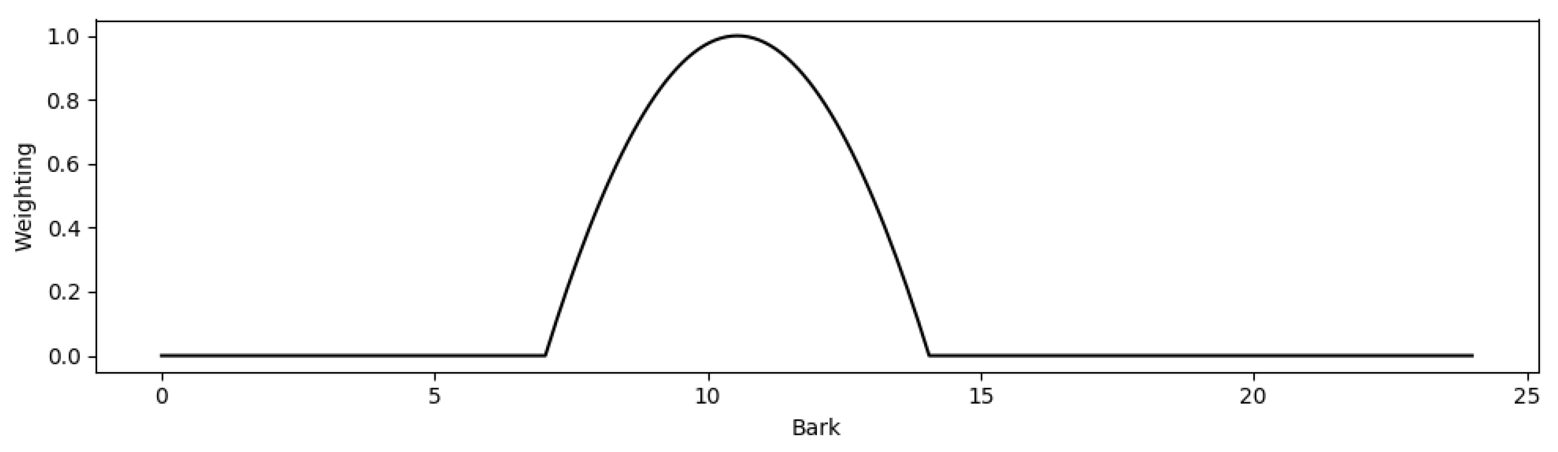
where is the specific loudness of the Bark band, and is a normal-distribution-shaped weighting function. The upper and lower limits of this weighting function were varied independently in steps of 1 Bark to determine the values that provided the greatest linear correlation between m and the mean listener ratings of hardness. The values thus chosen were 7 Bark (700 Hz) and 14 Bark (2150 Hz)—a lower frequency range than that used by Czedik-Eysenberg et al. [6,7]. The weighting function was calculated with the equation
where i is the Bark band and p is the normal distribution centred on 10.5 Bark, which is normalised between zero and one by taking the minimum value, and dividing by the range. This normal distribution is calculated with the equation
where is 0.01.
The weighting filter, , is shown graphically for 0 to 24 Bark in Figure 4.
This upper-midband level was calculated per 4096 samples and averaged across all time windows and not split by onsets. The mean and weighted-average was calculated over all time windows, using the RMS level of each window as weights.
3.7. Onset Strength and Logarithmic Transformations
Several of the described features are calculated per onset, and several of the stimuli contain multiple onsets. It is possible that the relative importance of each onset to the perceived hardness of the full stimulus is proportional to the perceptual prominence of that onset. The onset strength is a measure describing the prominence of an onset. This was used as the weighting factor in the calculation of a weighted-average for each per-onset feature, across all onsets within a stimulus.
Additionally, logarithmic transformation might improve the correlation of some of the suggested features, since human perception of frequency and amplitude are roughly logarithmic. To account for this, the base-10 logarithm of each feature was calculated.
4. Modelling Process
It is likely that several of the features account for the same variance in the listener ratings of hardness, and that others do not account for any variance. To develop a robust and generalisable model of hardness, features should only be included if they are necessary to account for variance within the data. Suitable features were chosen using an additive modelling method: initially creating a linear regression model with the one feature that best predicts the ratings of hardness, and iteratively adding the next-best performing feature. To avoid the use of multiple features describing similar variance within the data, potentially leading to an ungeneralisable model, the variance inflation factor (VIF) was calculated for each subsequent feature [33]. Myers [34] states that a VIF of greater than 10 is too large. Therefore, if the VIF of any feature is greater than 10 during the addition of any feature, this newly added feature was removed from inclusion in future iterations.
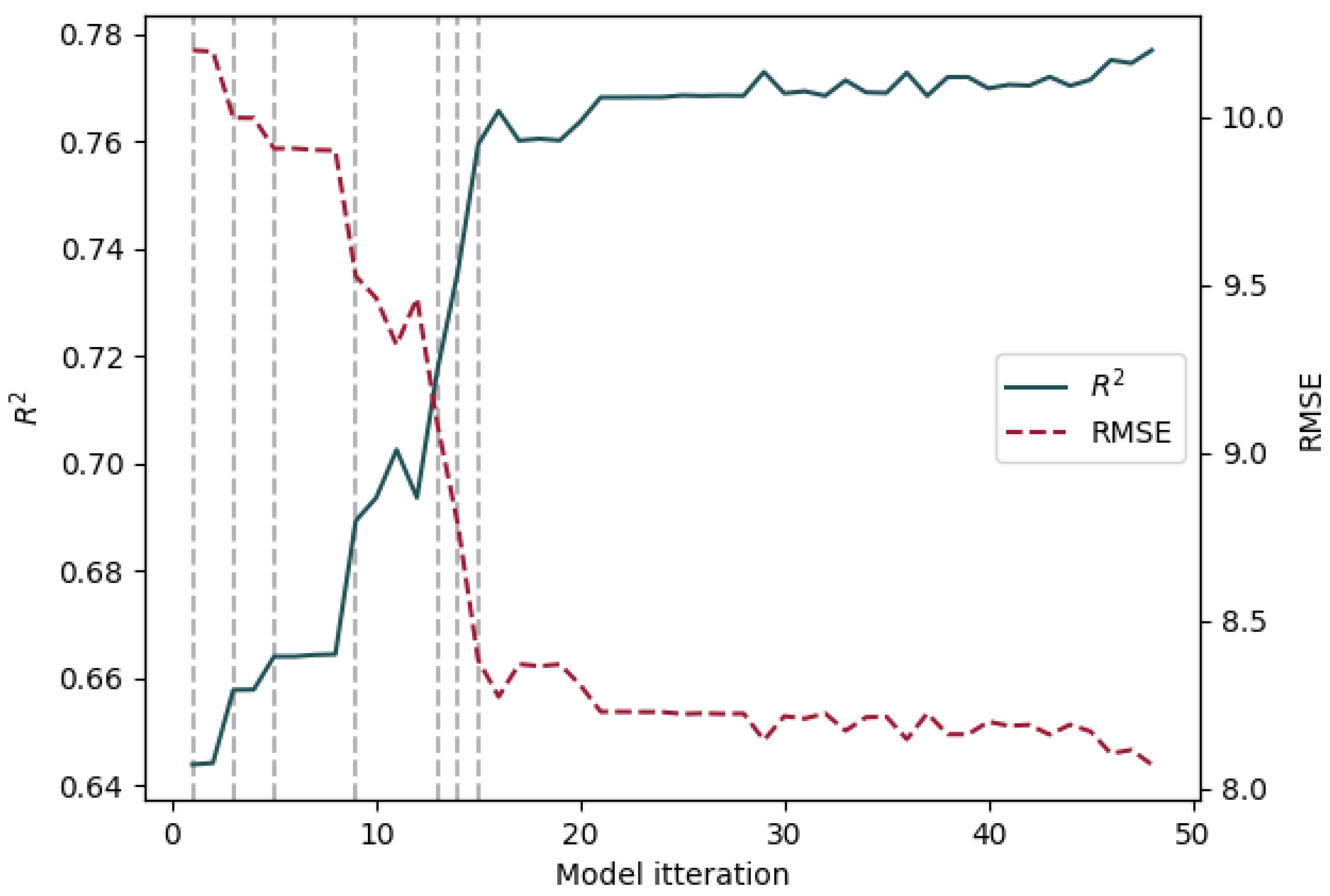
Figure 5 shows how the and root mean square error (RMSE) varied with each iteration. The performance generally increases with successive iterations, with several iterations offering a significant improvement, marked by grey vertical dashed lines. Several iterations where the model’s performance increases are not marked since the added feature was removed for violating the VIF criterion. The model’s performance appeared to stop improving after iteration 15, indicating that the features added beyond this point did not account for any additional variance in the data. The seven features added at the highlighted iterations are shown in Table 1, along with the model’s performance at that iteration.
From Table 1, the first two features that show an improvement of the hardness model are the logarithmic and linear version of the same feature: the weighted-average maximum bandwidth. The VIF metric used for removing features only tests whether a feature explains the same variance as a linear combination of other features; it cannot account for the nonlinear relationship between these two features. Therefore, the non-logarithmic-transformed version of this feature was removed from the final feature set. The final model of hardness is a multilinear regression of the log weighted average maximum bandwidth, the log mean attack centroid, the log weighted average midband level, the log percussive-to-harmonic ratio, the mean onset strength, and the log attack time.
Model Performance
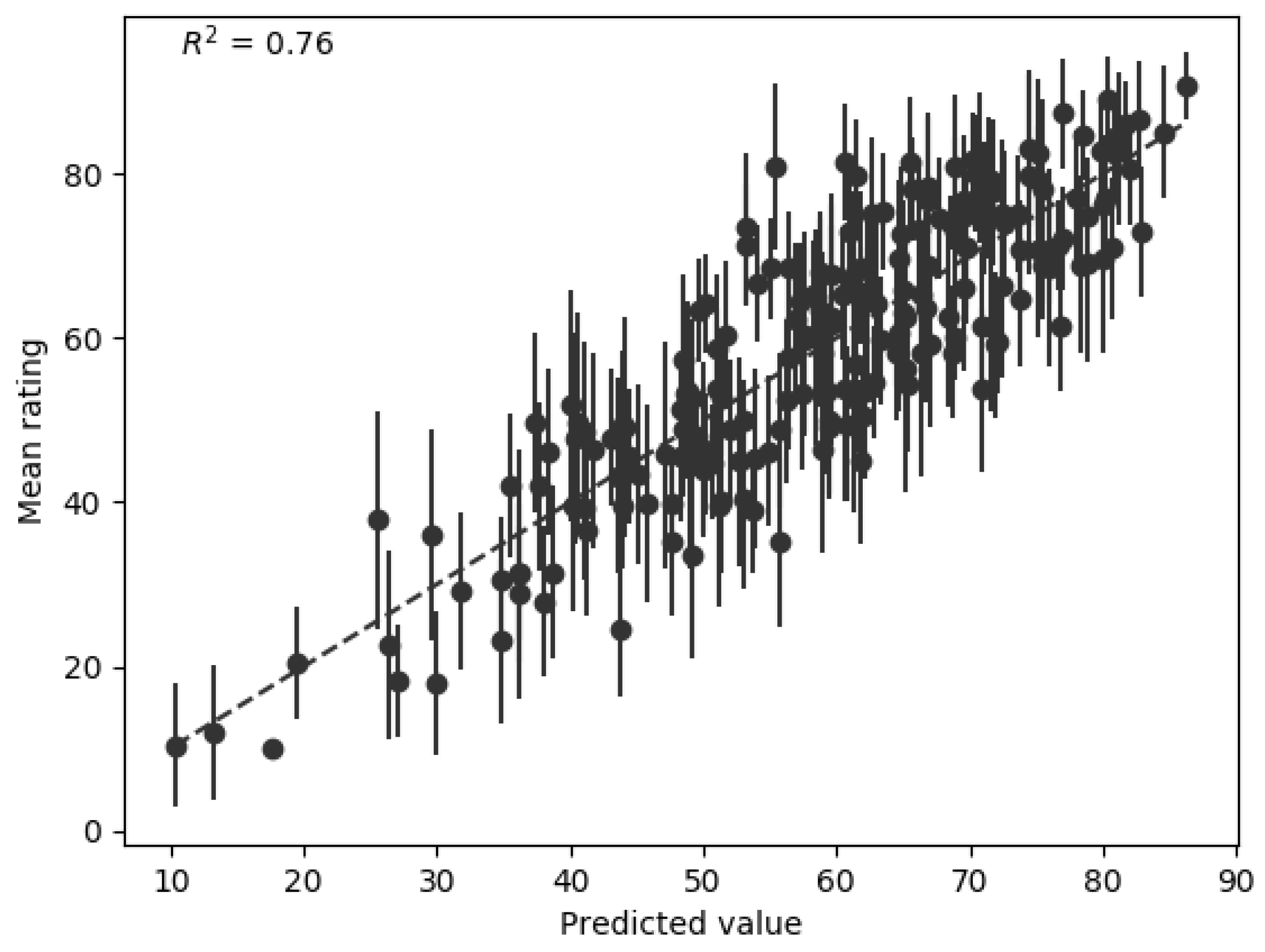
Figure 6 shows the performance of the final hardness model. This model achieves an of 0.76, and Spearman’s rho of 0.84. This compares favourably to the performance of Freed’s model ( = 0.725) and Czedik-Eysenberg et al.’s model ( = 0.723), especially given that the range of sounds used in the current research is very much wider than that used in either of the cited studies.
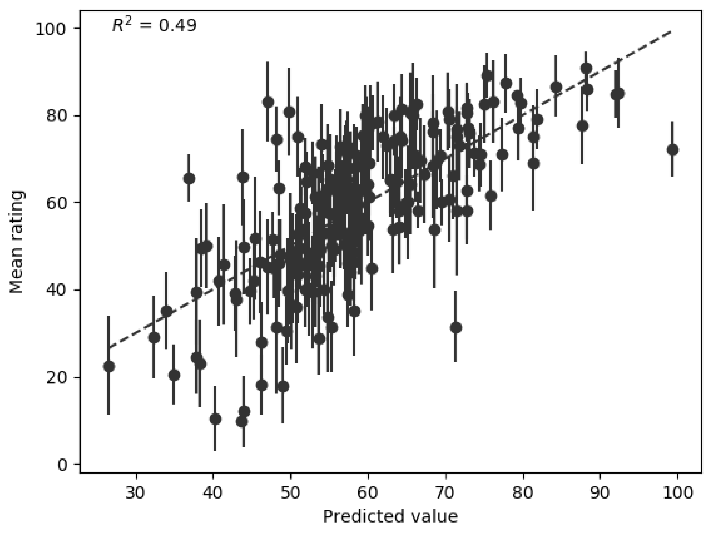
To further evaluate the performance of the final hardness model it was compared to a retrained version of Freed’s model: a linear regression model built from the four hardness features proposed by Freed [5] and trained on the listener ratings of hardness collected in the current study. The performance of this retrained Freed model is shown in Figure 7. The final hardness model outperforms the retrained Freed model, which achieved an of 0.49 and Spearman’s rho of 0.72. Figure 7 also shows that the retrained Freed model clusters many of its hardness predictions between 50 and 60.
5. Model Validation
The final hardness model can be considered generalisable if its prediction accuracy with a new (validation) dataset is similar to that achieved with the training dataset. Two validation datasets were created: one similar to the original training dataset where subjects rated the hardness of stimuli from multiple source types, called the between-source-type dataset; and a second dataset where the ratings of hardness were collected where subjects rated the hardness of the same source type, called the within-source-type dataset. This second dataset is relevant to a likely application of the model, where the user of an online sound-effect repository might search for sounds only of one particular type (e.g., kick drum) and wishes to sort the search results according to hardness.
To identify source types for the within-source-type validation dataset, the five most commonly searched source types identified in Section 2.1 were used: kick, piano, cymbal, snare, and guitar. For each source type, the acquisition method described in Section 2.2 was employed, but only five stimuli per source type were selected. The within-source-type listening tests were designed with the five stimuli of a single source type on each test page. To prevent scale compression effects, subjects were asked to use the full range of the scale on each test page.
The between-source-type validation dataset was compiled from stimuli gathered (using the same procedure) for related studies of each of the five other attributes (brightness, depth, reverb, metallic-nature, and roughness). The mid-rated stimulus for each source type for each of these attributes was used. These stimuli were supplemented with the mid-rated stimulus for each source type in the within-source-type hardness dataset. An independent expert then selected the most and least hard of these stimuli for use as hidden anchors on each test page. Each page of the between-source-type listening test had nine stimuli—the two hidden anchors and seven other stimuli randomly drawn from those remaining.
Both the within- and between-source-type listening tests were completed by a group of 16 subjects (14 male, 2 female, mean age = 21.1 ± 1.4 years), all of whom met the criteria set out in Section 2.3.
Note that the training and validation datasets did not incorporate common anchor stimuli, so the meanings of the “least hard” and “most hard” scale end-point labels will differ between datasets. Consequently the model’s performance should be evaluated in terms of linear correlation and rank order, and not in terms of absolute predicted hardness values.
5.1. Within-Source-Type Analysis
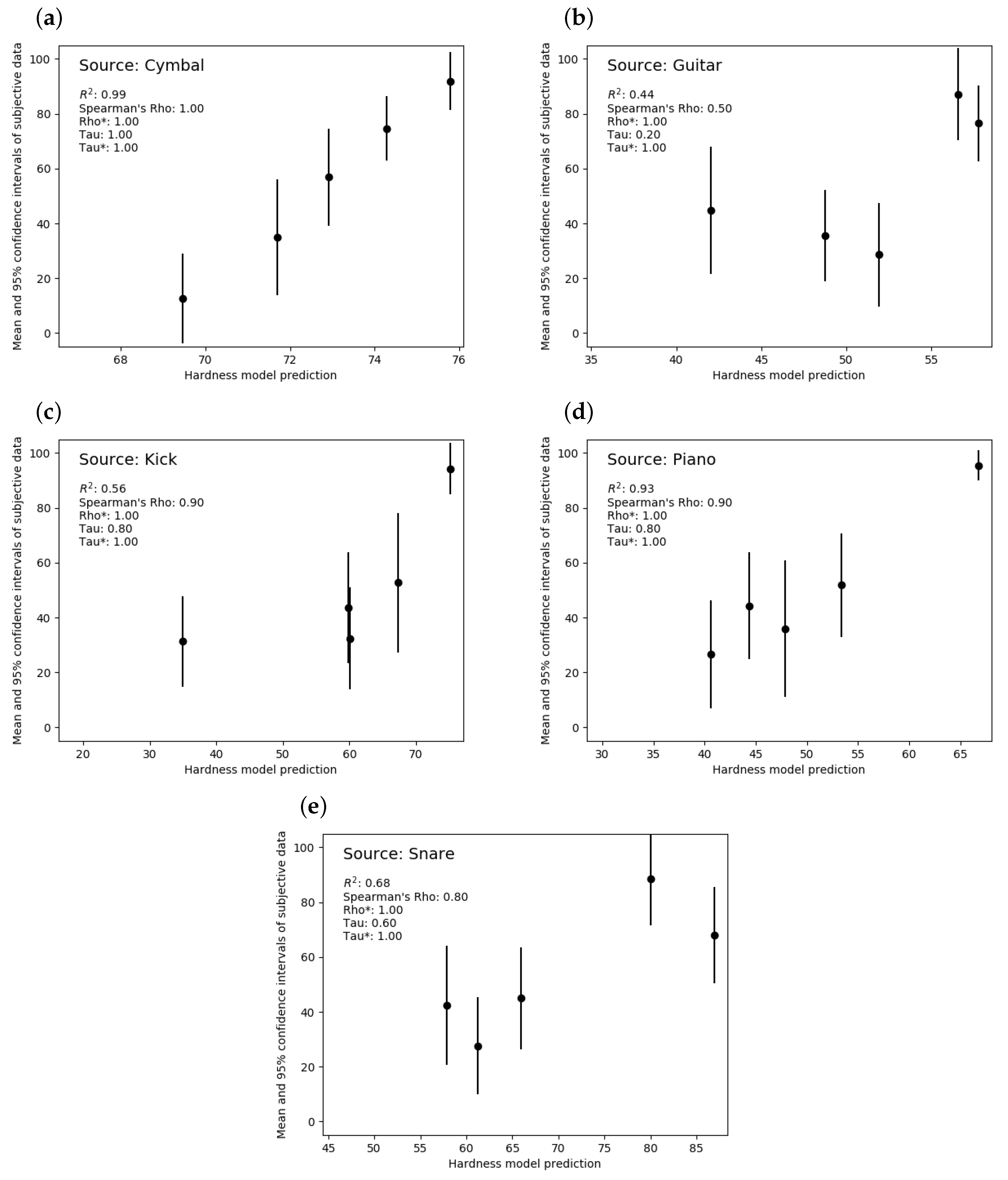
Figure 8 shows the performance of the developed hardness model with the five source types in the within-source-type test. Linear correlation between the model’s predictions and the listener ratings of hardness is assessed with . For the primary intended application of the model (filtering and sorting sound effect library search results), its ability to predict the rank order of hardnesses within a group of sounds is particularly important. Rank order accuracy is therefore also assessed, using Spearman’s rho and Kendall’s tau.
The model achieves a near-perfect linear correlation for the cymbal source type ( = 0.99), and high correlation for the piano and snare source types ( = 0.93 and = 0.68 respectively). The kick source type achieves a linear correlation of = 0.56, but from inspection of the plot it appears there is a nonlinear trend in the data. The guitar source type achieves the lowest correlation ( = 0.44). However, the general trend of the ratings is maintained: the two stimuli rated as the hardest with overlapping CI are predicted towards the top of the scale, whereas the three stimuli rated as least hard, also with overlapping CI, were predicted as less hard.
In terms of the rank order, the model predicts perfect rank order of the mean ratings with the cymbal and kick sources (rho = 1.0). With the piano and snare sources the model achieves high rank order correlations (rho = 0.90 and rho = 0.80 respectively), but scores the lowest with the guitar source type ( = 0.44, tau = 0.2). However, it is clear from these plots that there is notable variance in the subjective data, shown by the 95% confidence intervals (CI) considerably overlapping for adjacent results. To account for these when assessing the rank order of the models, the rho* and tau* metrics were calculated; manipulations of the Spearman’s rho and Kendall’s tau that take into consideration the variance in the subjective data [35]. Using these metrics, the model can predict the rank order perfectly, with rho* = 1.0 and tau* = 1.0 for all source types.
5.2. Between-Source-Type Analysis
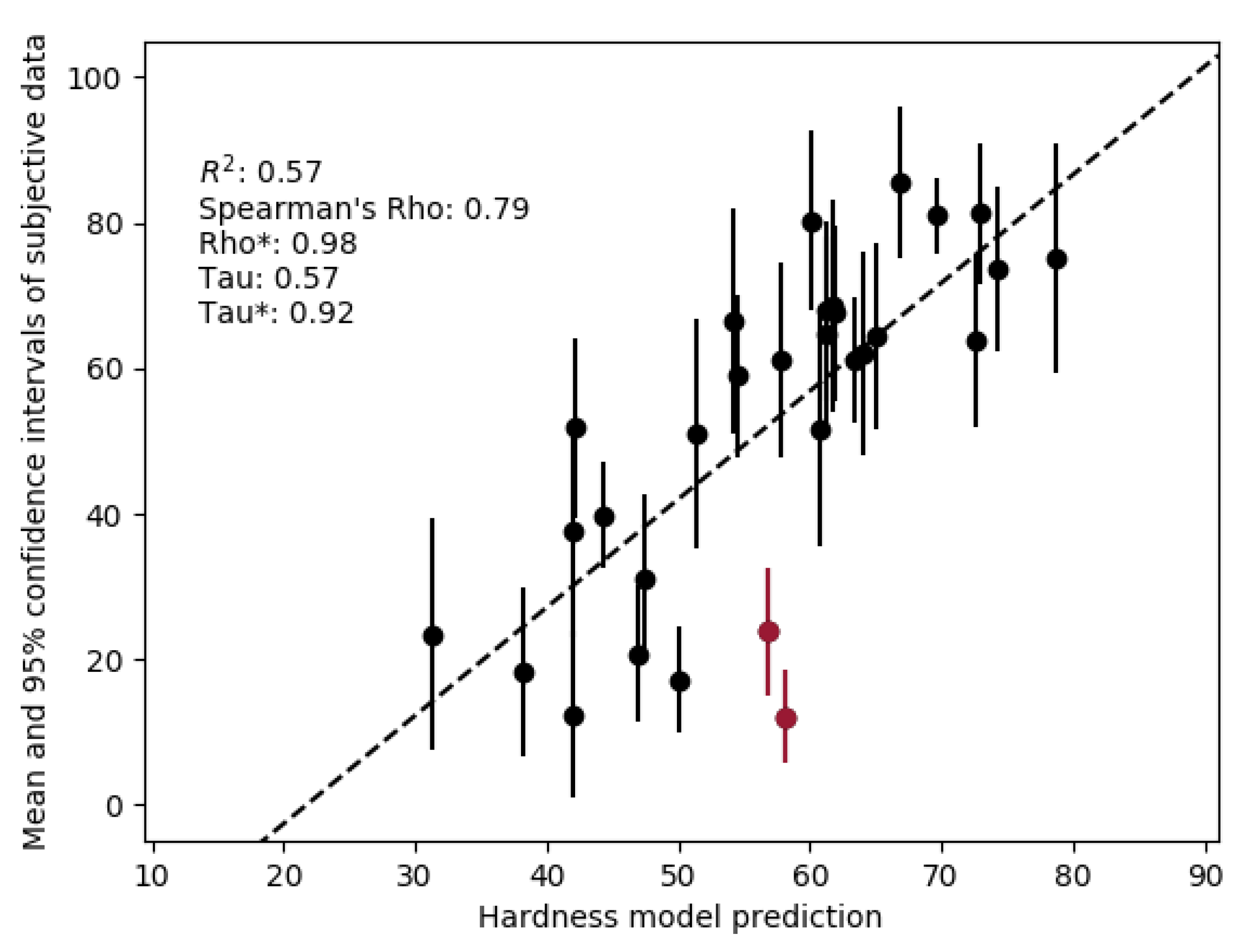
Figure 9 shows the performance of the hardness model with the between-source-type data.
When considering rank orders based purely on the mean ratings, the model achieves a Spearman’s rho of 0.79 and Kendall’s tau of 0.58. However, considering the subjective variance of the ratings, by examining rho* and tau*, the model achieves a performance of rho* = 0.98 and tau* = 0.92. For the linear correlation, the model achieves an of 0.57.
Two stimuli are highlighted in Figure 9. The hardness model over-predicted the hardness of these stimuli. Both of these stimuli were voices and had recording defects. One stimulus was particularly sibilant, which may account for the higher prediction of hardness, with this sibilant section potentially identified as an additional onset, resulting in higher than expected bandwidth and attack centroid. The other stimulus contained high levels of background noise and several clicks in the background. Listeners were possibly rating the perceived hardness of the voice only and internally filtering out the other sounds, whereas the implemented model of hardness may have identified these clicks as onsets and analysed them accordingly.
By removing these two highlighted stimuli, the model achieved a performance of = 0.69, rho = 0.83, rho* = 1.00, tau = 0.62, tau* = 0.97. This is similar to its performance with the training dataset and indicates that future development work might usefully target methods for handling low-quality recordings. This performance is also similar to that of standardised models such as PEAQ, which achieved = 0.68 [36].
6. Discussion
The developed model of hardness uses the features: log weighted average maximum bandwidth (b); mean attack centroid (c); log weighed-average midband level (m); log percussive-to-harmonic ratio (r); mean onset strength (s); and log attack time (a). The overall hardness can then be predicted with the linear regression:
Coefficients in Equation (9) are expressed to four significant figures and are non-standardised (each feature during the regression modelling was not standardised). This means that each feature’s coefficient can be directly implemented into a model of hardness, but does not indicate its relative contribution to hardness.
The majority of the variance in the data was explained by the log-weighted-average maximum bandwidth of the attack portion, the feature identified first in the iterative modelling process. This is a novel feature created by the authors. Similar previously explored bandwidth-related features, such as taking the difference between the spectral roll-on and roll-off, or the spectral spread [31], did not predict the perceived hardness well (nor did they relate to the authors impressions of bandwidth). The method described in this paper for calculating the bandwidth relies on a threshold method, and it is possible that some signals will never cross this threshold, resulting in an undetectable bandwidth. In this case the reported bandwidth defaults to the resolution of the frequency analysis (10.8 Hz) and might not reflect the actual signal bandwidth.
The log attack time of a sound has previously been proposed as a feature that relates to the softness of sounds [24]. This proposal was supported by the findings in this research: the log attack time improved the performance of the model; however, it should be noted that this feature was the last added and, therefore, does not account for the majority of the variance in the data.
Additionally, the model of timbral hardness developed in this study incorporates two features similar to features used in the musical hardness model developed by Czedik-Eysenberg et al. [6,7]. The percussive-to-harmonic ratio is calculated in a similar manner to the level of percussive energy feature in the musical hardness model. The midband level feature is similar to the intensity of signal components between 2 kHz and 4 kHz feature used in the musical hardness model, but focuses on a lower range of frequencies.
Using Freed’s four features (see Section 3.6) to create a linear regression model on the current dataset resulted in a performance of = 0.49 and rho = 0.72. The hardness model developed in this paper performs significantly better, = 0.76 and rho = 0.84. It should be noted that the stimuli used by Freed were controlled recordings of single impacts, where the variables were the type of mallet and object struck. This limited variation in the type of data that Freed’s model was trained on may explain its poorer performance with the current stimuli: sounds of multiple sources and unknown recording methods.
In the between-source-type validation, the hardness model achieved a performance of = 0.57 and rho = 0.79, lower than that obtained with the training data. As discussed in Section 4 and Section 5.2, technical deficiencies in the stimuli will impact the features extracted, yet may be ignored by subjects rating perceived hardness. It was shown that the performance of the model with the between-source-type validation data improves when removing signals with these degradations, increasing to 0.69, and rho to 0.83. Future development work might usefully target methods for handling low-quality recordings.
The motivation for the development of the hardness model, as set out in the introduction to this paper, was to allow the automated generation of hardness metadata to aid online sound effect repository searching. If the model can predict perceived hardness for a wide range of sound sources, with similar accuracy to that of a human, then it can be considered suitable for this application. To establish the accuracy of a human in this task, the correlation between each individual listener’s hardness ratings and the mean ratings across all listeners was calculated. The mean listener performance thus assessed was = 0.55, Spearman’s rho = 0.73. This makes the performance of the model (even without removal of problematic stimuli) slightly superior to that of the average human (in this study’s listening panel).
7. Conclusions
The search functionality of online sound effect repositories is limited by the quality and quantity of user-supplied metadata. It would therefore be beneficial if metadata could be generated automatically. In terms of timbral metadata, the most-searched term on the freesound.org repository is “hardness”. Previously, no perceptual model existed that could predict timbral hardness for a wide range of sound sources. The research documented in this paper aimed to develop a model that can do this.
With a training dataset of 202 stimuli, comprising hardness ratings of 36 source types, the developed model achieved an of 0.76 and Spearman’s rho of 0.84. With a new dataset, the model achieved an of 0.57 and Spearman’s rho of 0.79; allowing for subjective variance within the dataset produced rho* = 0.98 and tau* = 0.92. Inspection of several outlying stimuli suggested that deficiencies in the audio recordings may have led to over-prediction of hardness, with clicks and excessive sibilance captured by the model of hardness but potentially ignored by the listeners. Without these outliers, the model’s performance improved to = 0.69 and rho = 0.83, closer to its performance with the training dataset. With a further dataset, where listeners had directly compared the hardness of multiple sounds generated by a particular source type, the model achieved rho* and tau* of 1.0.
This model of hardness achieves similar performance to the PEAQ standardised model of audio quality assessment, and exceeds the performance of the average human (in this study’s listening panel). It is therefore suitable for use in the generation of hardness metadata and, indeed, has now been incorporated into the freesound.org website for this purpose, with its automatically generated metadata available through the freesound API. For the Audio Commons project, this will facilitate the use of CC-licensed audio by improving the search functionality available to repository users. Future research in this area could focus on (i) developing algorithms to detect recording deficiencies and identifying how these could be included in the model of hardness to improve the results; and/or (ii) developing models of other timbral attributes that may also be beneficial for filtering and sorting search results.
Author Contributions
Conceptualization, A.P., T.B. and R.M.; Data curation, A.P., T.B. and R.M.; Formal analysis, A.P.; Funding acquisition, T.B. and R.M.; Investigation, A.P.; Methodology, A.P., T.B. and R.M.; Project administration, T.B. and R.M.; Software, A.P.; Supervision, T.B. and R.M.; Validation, A.P.; Writing, original draft, A.P.; Writing, review & editing, A.P., T.B. and R.M.
Funding
This research was completed as part of the AudioCommons research project. This project has received funding from the European Union’s Horizon 2020 research and innovation programme under grant agreement No. 688382.
Conflicts of Interest
The authors declare no conflict of interest. The funders had no role in the design of the study; in the collection, analyses, or interpretation of data; in the writing of the manuscript, or in the decision to publish the results.
Abbreviations
The following abbreviations are used in this manuscript:
| CC | Creative Commons |
| RMS | Root Mean Square |
| VIF | Variance Inflation Factor |
| RMSE | Root Mean Square Error |
| CI | Confidence Interval |
References
- Bogdanov, D.; Wack, N.; Gómez Gutiérrez, E.; Gulati, S.; Herrera Boyer, P.; Mayor, O.; Roma Trepat, G.; Salamon, J.; Zapata González, J.R.; et al. ESSENTIA: An Audio Analysis Library for Music Information Retrieval. In Proceedings of the International Society for Music Information Retrieval Conference (ISMIR’13), Curitiba, Brazil, 4–8 November 2013; pp. 493–498. [Google Scholar]
- Plomp, R. A Review of Basic Research on Timbre. In Proceedings of the Symposium on Perception of Reproduced Sound; Stougaard Jensen: Copenhagen, Denmark, 1987. [Google Scholar]
- McAdams, S. Perspectives in the Contribution of Timbre to Musical Structure. Comput. Music J. 1999, 23, 85–102. [Google Scholar] [CrossRef]
- Howard, D.; Angus, J. Acoustics and Psychoacoustics, 2nd ed.; Focal Press: Oxford, UK, 2001; ISBN 9 78-0240521756. [Google Scholar]
- Freed, D. Auditory correlates of perceived mallet hardness for a set of recorded percussive sound events. J. Acoust. Soc. Am. 1990, 87, 311–322. [Google Scholar] [CrossRef] [PubMed]
- Czedik-Eysenberg, I.; Reuter, C.; Knauf, D. Decoding the sound of ‘hardness’ and ‘darkness’ as perceptual dimensions of music. In Proceedings of the 15th International Conference on Music Perception and Cognition/10th triennial conference of the European Society for the Cognitive Sciences of Music, Graz, Austria, 23–28 July 2018. [Google Scholar]
- Czedik-Eysenberg, I.; Knauf, D.; Reuter, C. Hardness as a semantic audio descriptor for music using automatic feature extraction. Informatik 2017. [Google Scholar] [CrossRef]
- Gabrielsson, A.; Sjȯgren, H. Perceived sound quality of sound-reproducing systems. J. Acoust. Soc. Am. 1979, 65, 1019–1033. [Google Scholar] [CrossRef] [PubMed]
- Lavandier, M.; Meunier, S.; Herzog, P. Identification of some perceptual dimensions underlying loudspeaker dissimilarities. J. Acoust. Soc. Am. 2008, 123, 4186–4198. [Google Scholar] [CrossRef] [PubMed]
- Michaud, P.; Lavandier, M.; Meunier, S.; Herzog, P. Objective characterization of perceptual dimensions underlying the sound reproduction of 37 single loudspeakers in a room. Acta Acust. Acust. 2015, 101, 603–615. [Google Scholar] [CrossRef]
- Aletta, F.; Kang, J.; Axelsson, Ö. Soundscape descriptors and a conceptual framework for developing predictive soundscape models. Landsc. Urban Plan. 2016, 149, 65–74. [Google Scholar] [CrossRef] [Green Version]
- Ma, K.; Wong, H.; Mak, C. A systematic review of human perceptual dimensions of sound: Meta-analysis of semantic differential method applications to indoor and outdoor sounds. Build. Environ. 2018, 133, 123–150. [Google Scholar] [CrossRef]
- Raimbault, M. Qualitative Judgements of Urban Soundscapes: Questioning Questionnaires and Semantic Scales. Acta Acust. Acust. 2006, 92, 929–937. [Google Scholar]
- Pearce, A.; Brookes, T.; Mason, R. Timbral attributes for sound effect library searching. In Proceedings of the Audio Engineering Society Conference: 2017 AES International Conference on Semantic Audio, Erlangen, Germany, 22–24 June 2017. [Google Scholar]
- Stĕpànek, J. Musical sound timbre: verbal description and dimensions. In Proceedings of the 9th International Conference on Digital Audio Effects, Montreal, QC, Canada, 18–20 September 2006. [Google Scholar]
- Giordano, B.; Petrini, K. Hardness recognition in synthetic sounds. In Proceedings of the Stockholm Music Acoustics Conference, Stockholm, Sweden, 6–9 August 2003. [Google Scholar]
- Giordano, B. Material categorization and hardness scaling in real and synthetic impact sounds. In The Sounding Object; Rocchesso, D., Fontana, F., Eds.; Mondo Estremo: Firenze, Italy, 2003. [Google Scholar]
- Zacharov, N.; Koivuniemi, K. Audio descriptive analysis & mapping of spatial sound displays. In Proceedings of the 2001 International Conference on Auditory Display, Espoo, Finland, 29 July–1 August 2001. [Google Scholar]
- Von Bismarck, G. Timbre of steady sounds: A factorial investigation of its verbal attributes. Acustica 1974, 30, 146–159. [Google Scholar]
- Martens, W.; Giragama, C. Relating multilingual semantic scales to a common timbre space. In Proceedings of the 113th Convention of the Audio Engineering Society, Los Angeles, CA, USA, 5–8 October 2002. [Google Scholar]
- Giragamal, C.; Martens, W.; Herath, S.; Wanasinghel, D.; Sabbirl, A. Relating multilingual semantic scales to a common timbre space—Part II. In Proceedings of the 115th Convention of the Audio Engineering Society, New York, NY, USA, 10–13 October 2003. [Google Scholar]
- Melara, R.; Marks, L. Interaction among auditory dimensions: Timbre, pitch, and loudness. Percept. Psychoacoust. 1990, 48, 169–178. [Google Scholar] [CrossRef] [Green Version]
- Le Bagousse, S.; Paquier, M.; Colomes, C. Categorization of Sound Attributes for Audio Quality Assessment—A Lexical Study. J. Audio Eng. Soc. 2014, 62, 736–747. [Google Scholar] [CrossRef]
- Williams, D.; Brookes, T. Perceptually-Motivated Audio Morphing: Softness. In Proceedings of the 126th Convention of the Audio Engineering Society, Munich, Germany, 7–10 May 2009. [Google Scholar]
- FFmpeg Developers. FFMPEG Tool (Version 3.4.1). Available online: http://ffmpeg.org/ (accessed on 16 March 2018).
- Schinkel-Bielefeld, N.; Lotze, N.; Nagel, F. Audio quality evaluation by experienced and inexperienced listeners. In Proceedings of the Meetings on Acoustics, Montreal, QC, Canada, 2–7 June 2013. [Google Scholar]
- Olive, S. Differences in Performance and Preference of Trained versus Untrained Listeners In Loudspeaker Tests: A Case Study. In Proceedings of the 114th Convention of the Audio Engineering Society, Amsterdam, The Netherlands, 22–25 March 2003. [Google Scholar]
- Bech, S.; Zacharov, N. Perceptual Audio Evaluation: Theory, Method and Application; Wiley: Chichester, UK, 2006; ISBN 978-0-470-86923-9. [Google Scholar]
- Tomic, O.; Luciano, G.; Nilsen, A.; Hyldig, G.; Lorensen, K.; Næs, T. Analysing sensory panel performance in proficiency tests using the PanelCheck software. Eur. Food Res. Technol. 2010, 230, 497–511. [Google Scholar] [CrossRef]
- McFee, B.; McVicar, M.; Raffel, C.; Liang, D.; Nieto, O.; Moore, J.; Ellis, D.; Repetto, D.; Viktorin, P.; Santos, J.F.; et al. Librosa: v0.4.0. Zenodo 2015. [Google Scholar] [CrossRef]
- Peeters, G. A Large Set of Audio Features for Sound Description (Similarity and Classification) in the CUIDADO Project; Technical report; Institut de Recherche Et Coordination Acoustique/Musique: Paris, France, 2004. [Google Scholar]
- Fastl, E.; Zwicker, H. Psychoacoustics, Facts and Models; Springer: Berlin, Germnay, 1991; ISBN 3-540-65063-6. [Google Scholar]
- Weisberg, S. Applied Linear Regression; Wiley: Chichester, UK, 1985; ISBN 978-1-118-38608-8. [Google Scholar]
- Mysers, R. Classical and Modern Regression With Applications; Duxbury Press: Belmont, TN, USA, 1990; ISBN 978-0534380168. [Google Scholar]
- Pearce, A.; Isabelle, S.; Francois, H.; Oh, E. Methods of Assessing the Rank Order of Prediction Models with Respect to Variance of Listening Test Ratings. J. Audio Eng. Soc. 2019, in press. [Google Scholar]
- ITU-R BS.1387-1. ITU-R BS.1387-1 Method for Objective Measurements of Perceived Audio Quality; International Telecommunications Union: Geneva, Switzerland, 2001. [Google Scholar]
Sample Availability: The data underlying the findings presented in this paper are available from doi:10.5281/zenodo.1548721. Further project information can be found at http://www.audiocommons.org. |
Figure 1.
The interface used for selecting stimuli.

Figure 2.
The listening test interface.

Figure 3.
Plan view of listening test rooms. Hashed areas represent acoustically absorbent panels. A fourth panel, 1.25 m by 2.0 m, was attached to the ceiling in the centre of the room. Height refers to the floor-to-ceiling distance, ignoring the fourth acoustic panel.
Figure 3.
Plan view of listening test rooms. Hashed areas represent acoustically absorbent panels. A fourth panel, 1.25 m by 2.0 m, was attached to the ceiling in the centre of the room. Height refers to the floor-to-ceiling distance, ignoring the fourth acoustic panel.

Figure 4.
Weighting function for midband frequencies.

Figure 5.
Performance of the multilinear regression model for each stage of the iterative modelling. The dashed grey lines represent iterations where the model shows marked improvement.
Figure 5.
Performance of the multilinear regression model for each stage of the iterative modelling. The dashed grey lines represent iterations where the model shows marked improvement.

Figure 6.
Performance of the final hardness model with the training dataset.

Figure 7.
Performance of a linear regression model based only on the features proposed by Freed [5].
Figure 7.
Performance of a linear regression model based only on the features proposed by Freed [5].

Figure 8.
Performance of the hardness model with the within-source-type validation data. (a) Cymbal. (b) Guitar. (c) Kick. (d) Piano. (e) Snare.
Figure 8.
Performance of the hardness model with the within-source-type validation data. (a) Cymbal. (b) Guitar. (c) Kick. (d) Piano. (e) Snare.

Figure 9.
Performance of the hardness model with the between-source-type validation data.


Table 1.
Performance of the features that show improved performance during the iterative modelling process.
Table 1.
Performance of the features that show improved performance during the iterative modelling process.
| Iteration Number | Feature | RMSE | |
|---|---|---|---|
| 1 | log weighted-average maximum bandwidth | 0.64 | 10.20 |
| 3 | weighted-average maximum bandwidth | 0.66 | 10.00 |
| 5 | log mean attack centroid | 0.66 | 9.91 |
| 9 | log weighed average midband level | 0.69 | 9.53 |
| 13 | log percussive-to-harmonic ratio | 0.72 | 9.08 |
| 14 | mean onset strength | 0.74 | 8.79 |
| 15 | log attack time | 0.76 | 8.38 |
© 2019 by the authors. Licensee MDPI, Basel, Switzerland. This article is an open access article distributed under the terms and conditions of the Creative Commons Attribution (CC BY) license (http://creativecommons.org/licenses/by/4.0/).
Share and Cite
MDPI and ACS Style
Pearce, A.; Brookes, T.; Mason, R. Modelling Timbral Hardness. Appl. Sci. 2019, 9, 466. https://0-doi-org.brum.beds.ac.uk/10.3390/app9030466
AMA Style
Pearce A, Brookes T, Mason R. Modelling Timbral Hardness. Applied Sciences. 2019; 9(3):466. https://0-doi-org.brum.beds.ac.uk/10.3390/app9030466
Chicago/Turabian StylePearce, Andy, Tim Brookes, and Russell Mason. 2019. "Modelling Timbral Hardness" Applied Sciences 9, no. 3: 466. https://0-doi-org.brum.beds.ac.uk/10.3390/app9030466
Note that from the first issue of 2016, this journal uses article numbers instead of page numbers. See further details here.