Author Contributions
Conceptualization, R.-B.C., F.B., P.N. and F.S.; methodology, R.-B.C., F.B., P.N. and F.S.; software, R.-B.C., F.B. and P.N.; validation, R.-B.C., F.B., P.N., F.D.M. and F.S.; resources, F.B., F.D.M. and P.N.; data curation, R.-B.C. and F.B.; writing, original draft preparation R.-B.C. and F.B.; writing, review and editing, R.-B.C., F.B., F.D.M., P.N. and F.S.; funding acquisition, F.B. and F.D.M.
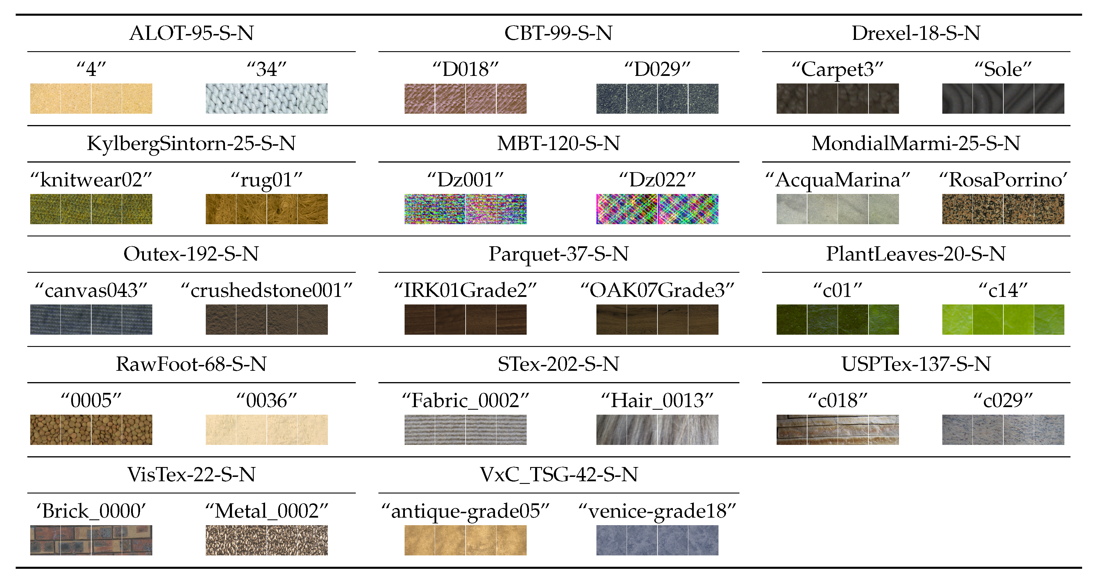
Figure 1.
Group #1: Stationary textures acquired under steady imaging conditions (
Section 3.2.1).
Figure 1.
Group #1: Stationary textures acquired under steady imaging conditions (
Section 3.2.1).
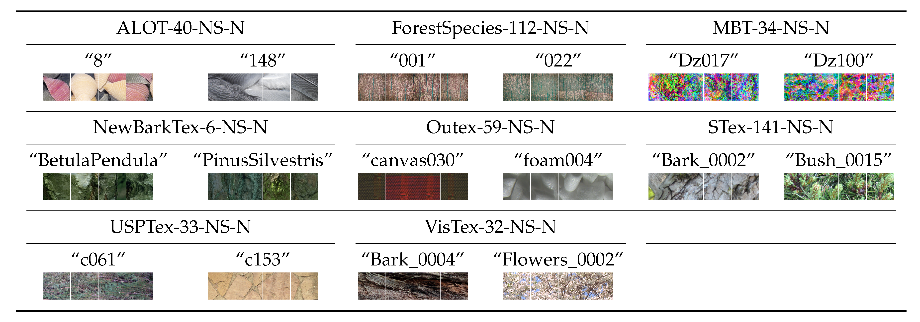
Figure 2.
Group #2: Non-stationary textures acquired under steady imaging conditions (
Section 3.2.2).
Figure 2.
Group #2: Non-stationary textures acquired under steady imaging conditions (
Section 3.2.2).
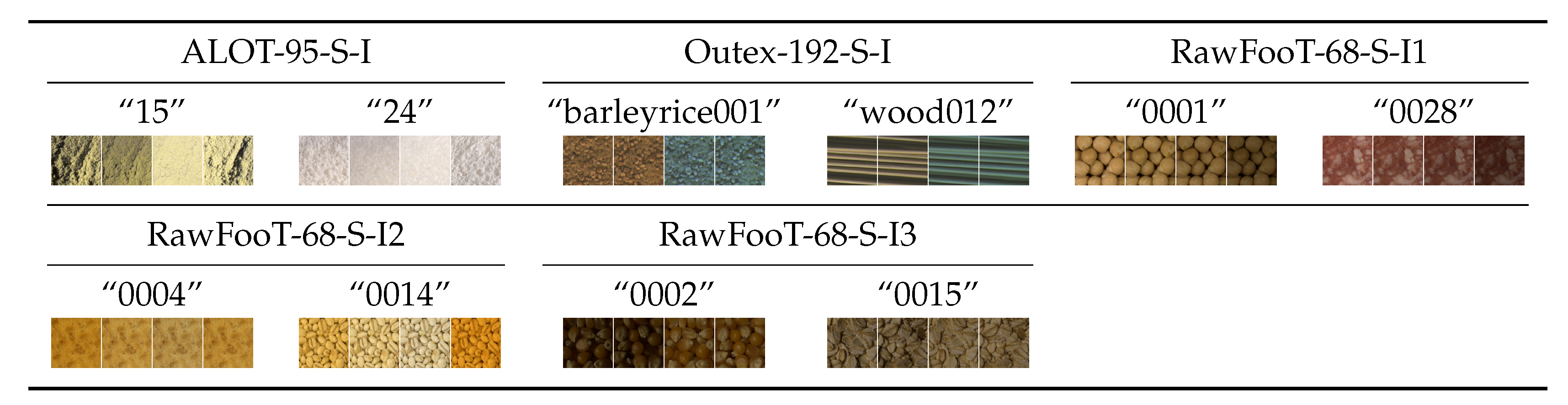
Figure 3.
Group #3: Stationary textures acquired under variable illumination (
Section 3.2.3).
Figure 3.
Group #3: Stationary textures acquired under variable illumination (
Section 3.2.3).
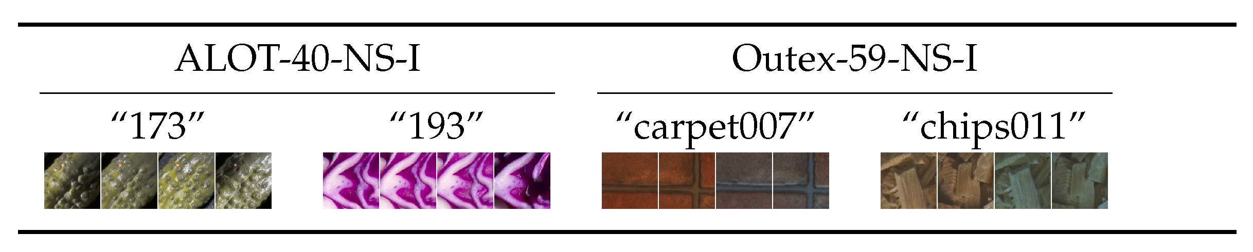
Figure 4.
Group #4: Non-stationary textures acquired under variable illumination (
Section 3.2.4).
Figure 4.
Group #4: Non-stationary textures acquired under variable illumination (
Section 3.2.4).
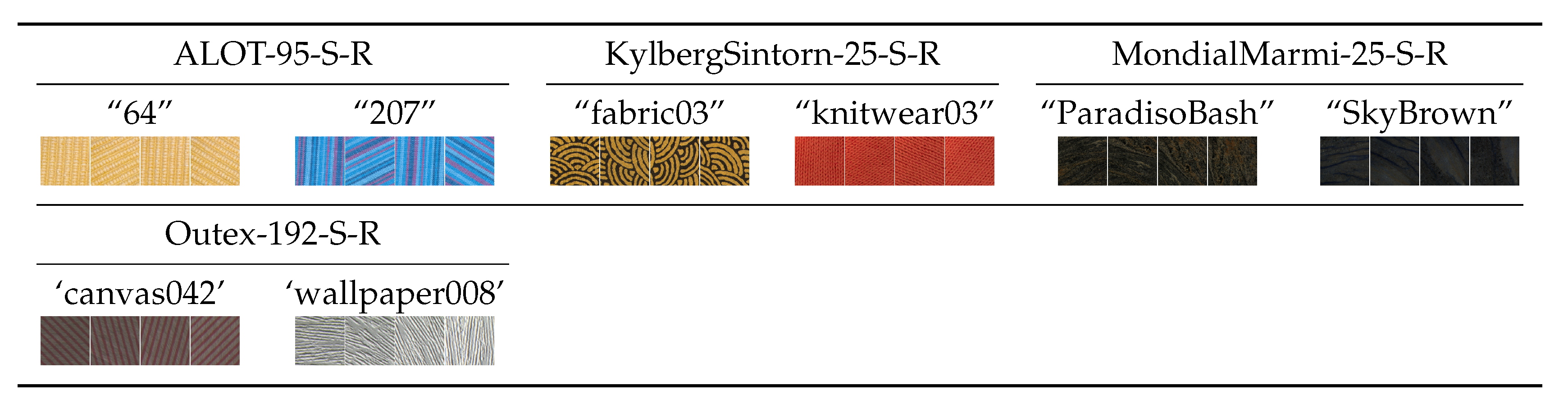
Figure 5.
Group #5: Stationary textures with rotation (
Section 3.2.5).
Figure 5.
Group #5: Stationary textures with rotation (
Section 3.2.5).
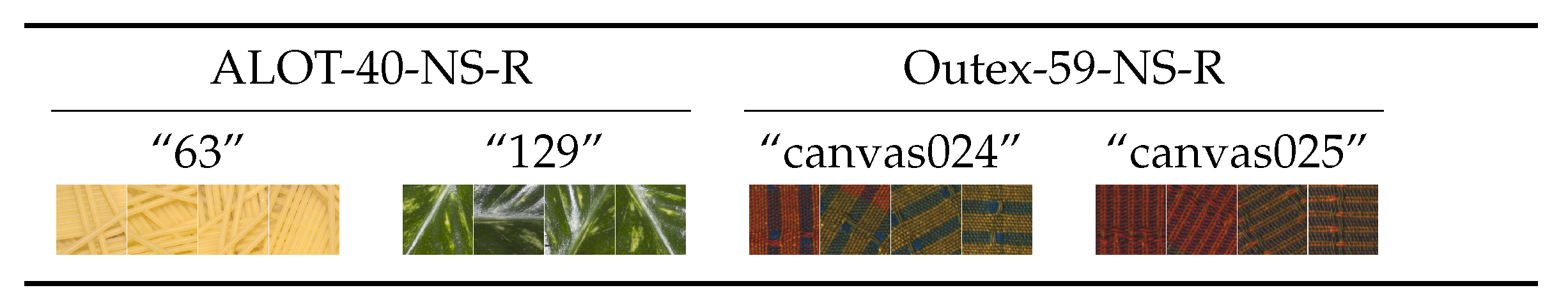
Figure 6.
Group #6: Non-stationary textures with rotation (
Section 3.2.6).
Figure 6.
Group #6: Non-stationary textures with rotation (
Section 3.2.6).
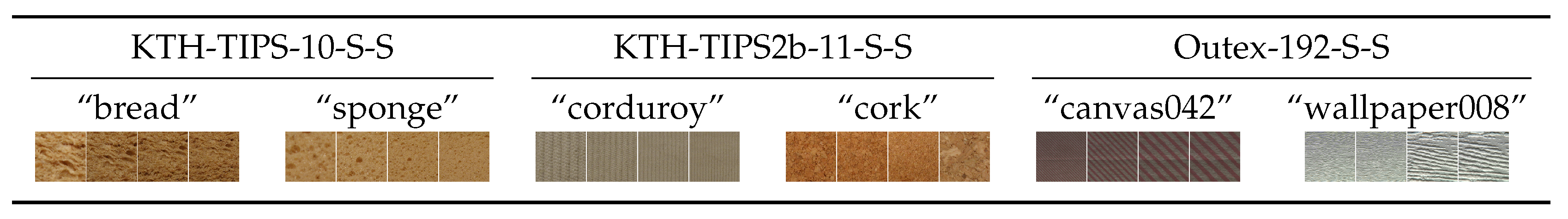
Figure 7.
Group #7: Stationary textures with variations in scale (
Section 3.2.7).
Figure 7.
Group #7: Stationary textures with variations in scale (
Section 3.2.7).
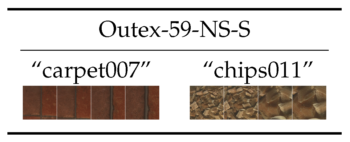
Figure 8.
Group #8: Non-stationary textures with variations in scale (
Section 3.2.8).
Figure 8.
Group #8: Non-stationary textures with variations in scale (
Section 3.2.8).
Figure 9.
Group #9: Stationary textures acquired under multiple variations in the imaging conditions (
Section 3.2.9).
Figure 9.
Group #9: Stationary textures acquired under multiple variations in the imaging conditions (
Section 3.2.9).
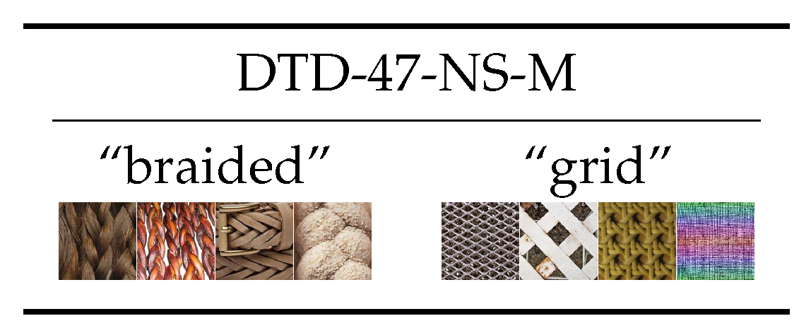
Figure 10.
Group #10: Non-stationary textures acquired under multiple variations in the imaging conditions (
Section 3.2.10).
Figure 10.
Group #10: Non-stationary textures acquired under multiple variations in the imaging conditions (
Section 3.2.10).
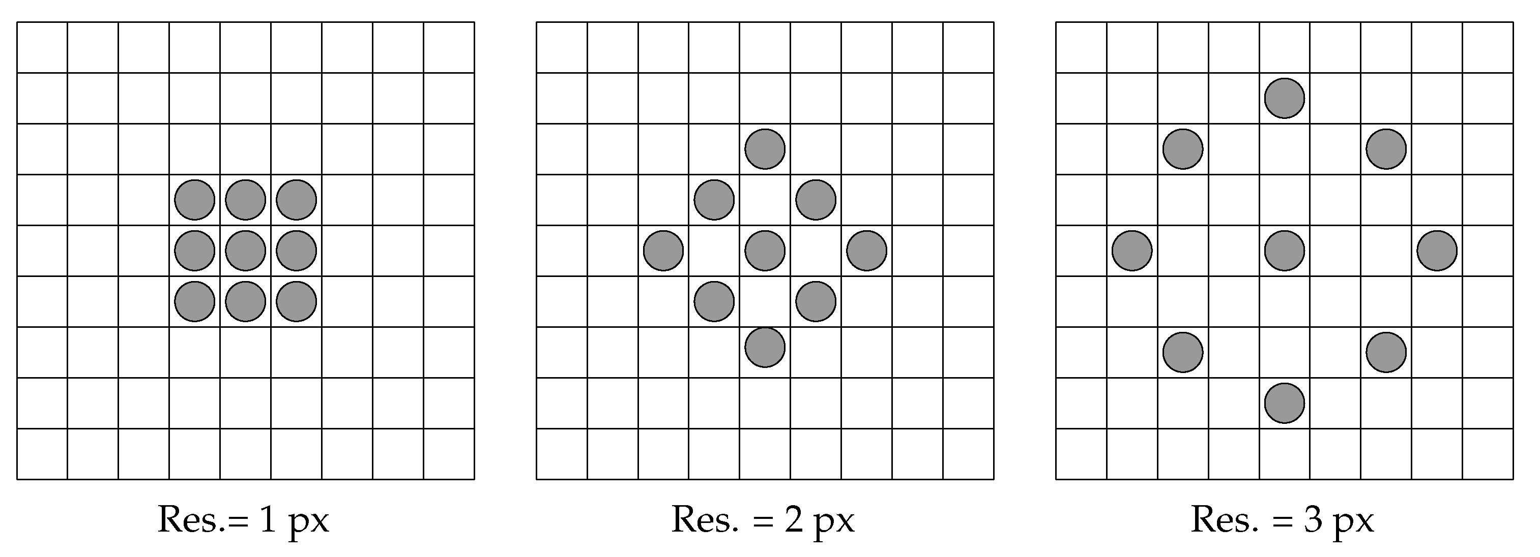
Figure 11.
Neighbourhoods used to compute features through histograms of equivalent patterns and other methods.
Figure 11.
Neighbourhoods used to compute features through histograms of equivalent patterns and other methods.
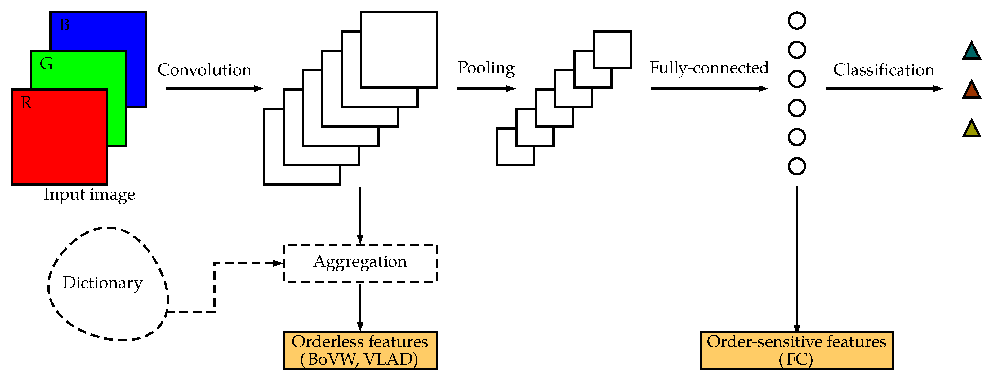
Figure 12.
Simplified diagram of a generic convolutional neural network. For texture classification, we can either use the order-sensitive output of a fully-connected layer or the orderless, aggregated output of a convolutional layer.
Figure 12.
Simplified diagram of a generic convolutional neural network. For texture classification, we can either use the order-sensitive output of a fully-connected layer or the orderless, aggregated output of a convolutional layer.
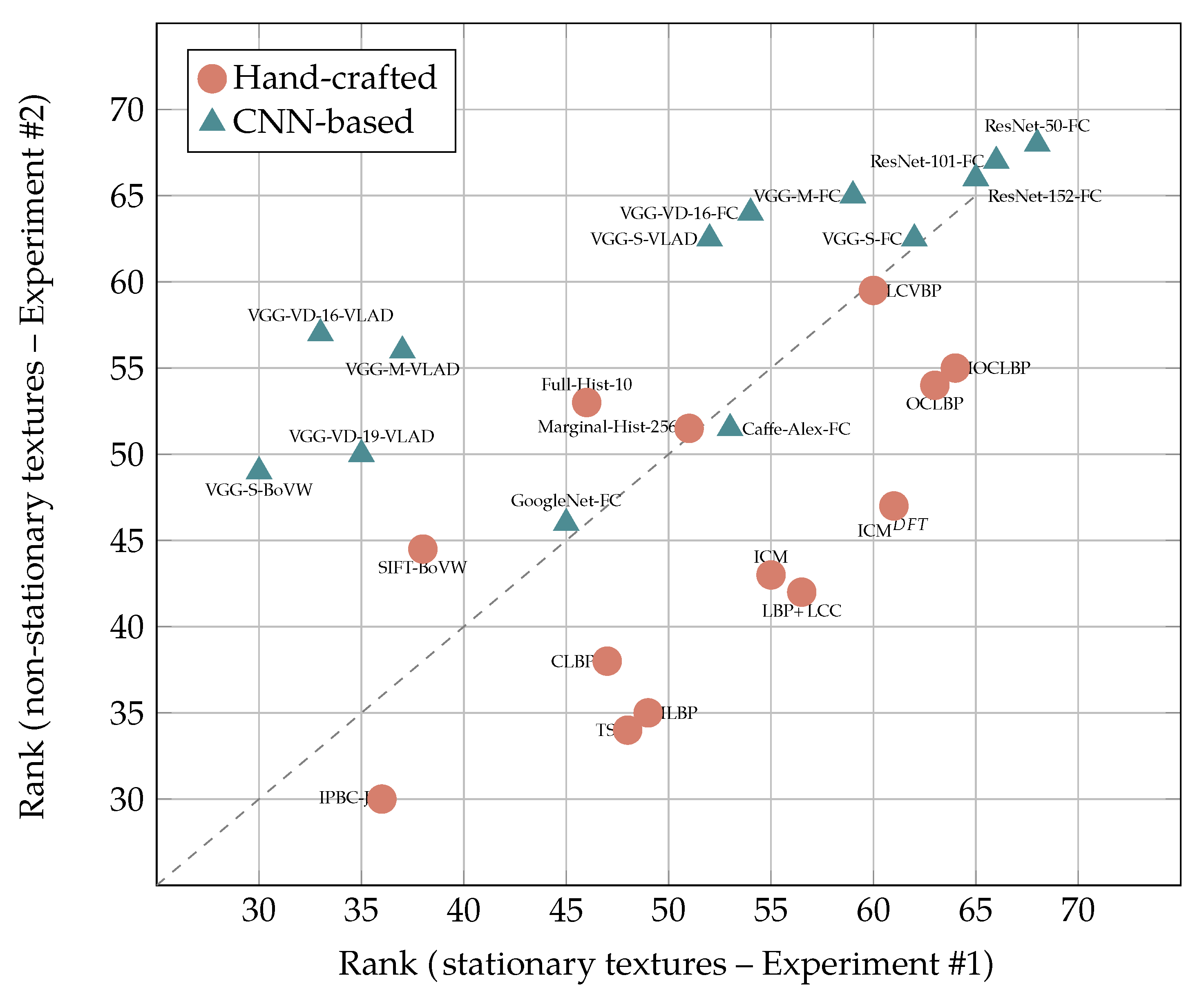
Figure 13.
Relative performance of hand-crafted descriptors vs. CNN-based features with stationary (x axis) and non-stationary textures (y axis) under invariable imaging conditions (Experiments #1 and #2, best 13 methods). The plot shows a clear divide between CNN-based methods (mostly clustered in the upper-left part, therefore showing affinity for non-stationary textures) and hand-crafted descriptors (mostly clustered in the lower-right part, therefore showing affinity for stationary textures)
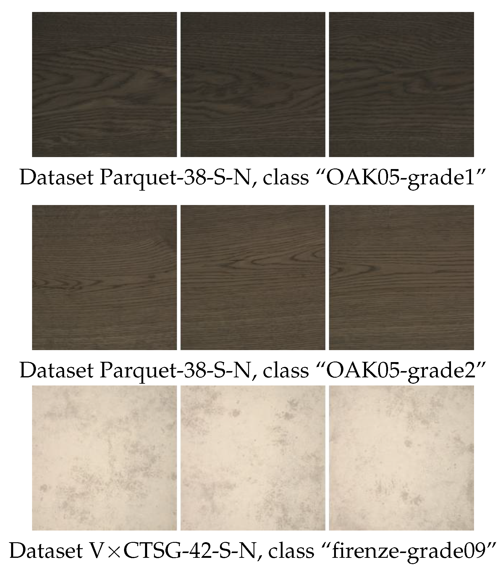
Figure 14.
Hand-crafted image descriptors proved generally better than CNN-based features for the classification of stationary textures acquired under invariable imaging conditions. The gap was substantial when it came to discriminating between very similar textures, as those shown in the picture.
Figure 14.
Hand-crafted image descriptors proved generally better than CNN-based features for the classification of stationary textures acquired under invariable imaging conditions. The gap was substantial when it came to discriminating between very similar textures, as those shown in the picture.
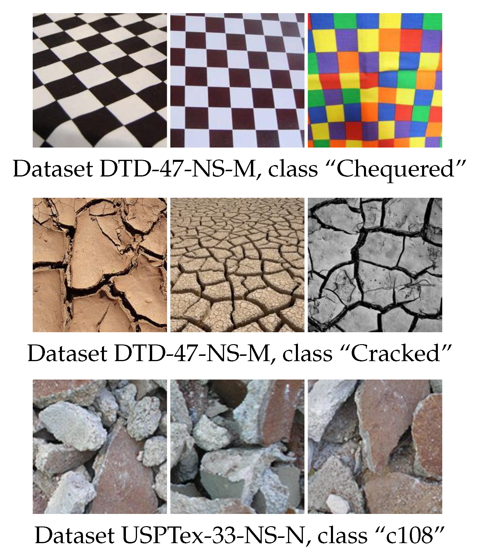
Figure 15.
CNN-based features were on the whole better than hand-crafted descriptors at classifying non-stationary textures, as those shown in the picture.
Figure 15.
CNN-based features were on the whole better than hand-crafted descriptors at classifying non-stationary textures, as those shown in the picture.
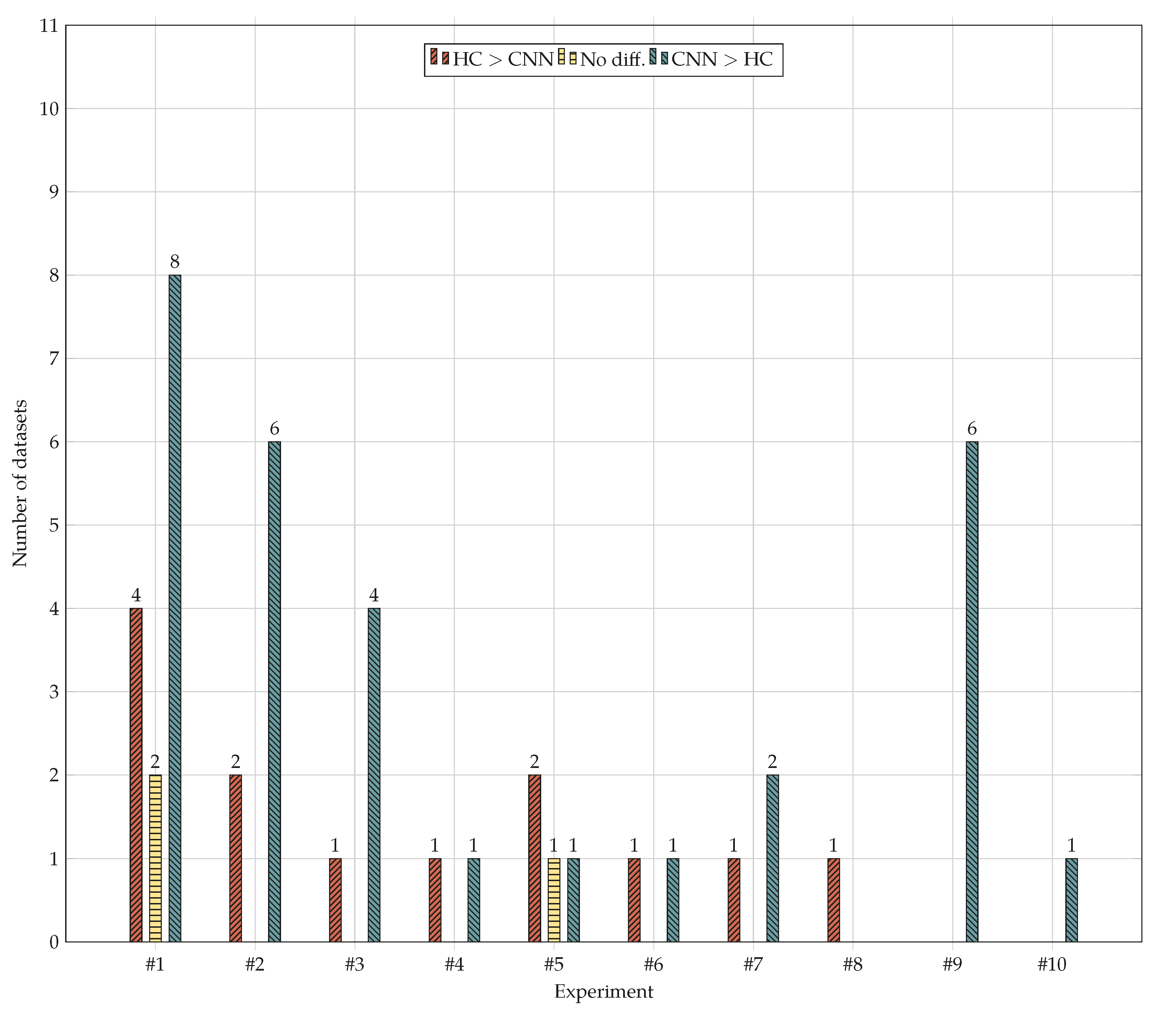
Figure 16.
Number of datasets on which: hand-crafted methods performed significantly better than CNNs (“HC > CNN”); there was no significant difference (“No diff.”) and CNNs performed significantly better than hand-crafted methods (“CNN > HC”). see also
Table 6,
Table 7,
Table 8,
Table 9,
Table 10,
Table 11,
Table 12 and
Table 13.
Table 1.
Round-up table of the image datasets used in the experiments. ALOT, Amsterdam Library of Textures; CUReT, Columbia-Utrecht Reflectance and Texture Database; CBT, Coloured Brodatz Textures; MBT, Multiband Texture Database; RawFooT, Raw Food Texture Database; VisTex, Vision Texture Database; RDAD, Robotics Domain Attribute Database; STex, Salzburg Texture Image Database; DTD, Describable Texture Dataset; S, Stationary; NS, Non-Stationary; N, No variations; I, variations in Illumination; R, variations in Rotation; S, variations in Scale, M, Multiple variations.
| VARIATIONS IN THE IMAGING CONDITIONS |
|---|
| TYPE OF TEXTURE | | NONE | ILLUMINATION | ROTATION | SCALE | MULTIPLE VARIATIONS |
| | Group 1 | Group 3 | Group 5 | Group 7 | Group 9 |
| STATIONARY | ALOT-95-S-N | ALOT-95-S-I | ALOT-95-S-R | KTH-TIPS-10-S-S | CUReT-61-S-M |
| CBT-99-S-N | Outex-192-S-I | KylbergSintorn-25-S-R | KTH-TIPS2b-11-S-S | Fabrics-1968-S-M |
| Drexel-18-S-N | RawFooT-68-S-I1 | MondialMarmi-25-S-R | Outex-192-S-S | KTH-TIPS-10-S-M |
| KylbergSintorn-25-S-N | RawFooT-68-S-I2 | Outex-192-S-R | | KTH-TIPS2b-11-S-M |
| MBT-120-S-N | RawFooT-68-S-I3 | | | LMT-94-S-M |
| MondialMarmi-25-S-N | | | | RDAD-27-S-M |
| Outex-192-S-N | | | | |
| Parquet-38-S-N | | | | |
| PlantLeaves-20-S-N | | | | |
| RawFooT-68-S-N | | | | |
| STex-202-S-N | | | | |
| USPTex-137-S-N | | | | |
| VisTex-89-S-N | | | | |
| VxC_TSG-42-S-N | | | | |
| | Group 2 | Group 4 | Group 6 | Group 8 | Group 10 |
| NON-STATIONARY | ALOT-40-NS-N | ALOT-40-NS-I | ALOT-40-NS-R | Outex-59-NS-S | DTD-47-NS-M |
| ForestSpecies-112-NS-N | Outex-59-NS-I | Outex-59-NS-R | | |
| MBT-34-NS-N | | | | |
| NewBarkTex-6-NS-N | | | | |
| Outex-59-NS-N | | | | |
| STex-138-NS-N | | | | |
| USPTex-33-NS-N | | | | |
| VisTex-78-NS-N | | | | |
Table 2.
Summary table of the hand-crafted image descriptors used in the experiments. VLAD, Vectors of Locally-Aggregated Descriptors.
Table 2.
Summary table of the hand-crafted image descriptors used in the experiments. VLAD, Vectors of Locally-Aggregated Descriptors.
| Method | Variant | Abbreviation | No. of Features |
|---|
| Purely spectral descriptors |
| Mean of each channel | | Mean | 3 |
| Mean and std. dev.of each channel | | Mean + Std | 6 |
| Mean and moms.from 2th to 5th of each ch. | | Mean + Moms | 15 |
| Quartiles of each channel | | Quartiles | 9 |
| 256-bin Marginal Histogram of each channel | | Marginal-Hists-256 | 768 |
| 10-bin joint colour Histogram | | Full-Hist-10 | 1000 |
| Grey-scale texture descriptors |
| Completed Local Binary Patterns | Rotation-invariant | CLBP | 324 |
| Gradient-based Local Binary Patterns | Rotation-invariant | GLBP | 108 |
| Improved Local Binary Patterns | Rotation-invariant | ILBP | 213 |
| Local Binary Patterns | Rotation-invariant | LBP | 108 |
| Local Ternary Patterns | Rotation-invariant | LTP | 216 |
| Texture Spectrum | Rotation-invariant | TS | 2502 |
| Grey-level Co-occurrence Matrices | | GLCM | 60 |
| Grey-level Co-occurrence Matrices | | GLCM | 60 |
| Gabor features | | Gabor | 70 |
| Gabor features | Rotation-invariant | Gabor | 70 |
| Gabor features | Contrast-normalised | Gabor | 70 |
| Gabor features | Rot.-inv.and ctr.-norm. | Gabor | 70 |
| Image Patch-Based Classifier | Joint | IPBC-J | 4096 |
| Histograms of Oriented Gradients | | HOG | 768 |
| Dense SIFT | BoVW aggregation | SIFT-BoVW | 4096 |
| Dense SIFT | VLAD aggregation | SIFT-VLAD | 4608 |
| VZClassifier | MR8filters | VZ-MR8 | 4096 |
| Wavelet Statistical and Co-occurrence Features | Haar wavelet | WSF + WCF | 84 |
| Wavelet Statistical and Co-occurrence Features | Bi-orthogonal wavelet | WSF + WCF | 84 |
| Colour texture descriptors |
| Improved Opponent Colour LBP | Rotation-invariant | IOCLBP | 1287 |
| Integrative Co-occurrence Matrices | | ICM | 360 |
| Integrative Co-occurrence Matrices | Rotation-invariant | ICM | 360 |
| Local Binary Patterns + Local Colour Contrast | Rotation-invariant LBP | LBP + LCC | 876 |
| Local Colour Vector Binary Patterns | Rotation-invariant | LCVBP | 432 |
| Opponent Colour Local Binary Patterns | Rotation-invariant | OCLBP | 648 |
| Opponent Gabor features | | OppGabor | 630 |
| Opponent Gabor features | Contrast-normalised | OppGabor | 630 |
| Opponent Gabor features | Rotation-onvariant | OppGabor | 630 |
| Opponent Gabor features | Rot.-inv. and ctr.-norm. | OppGabor | 630 |
Table 3.
Summary table of the off-the-shelf CNN-based features used in the experiments.
Table 3.
Summary table of the off-the-shelf CNN-based features used in the experiments.
| Pre-Trained Model | Output Layer (No. or Name) | Aggregation Method | Abbreviation | No. of Features |
|---|
| DenseNet_161.caffemodel | “pool5” (last Fully-Conn.) | None | DenseNet-161-FC | 2208 |
| DenseNet_161.caffemodel | “concat_5_24” (last conv.) | BoVW | DenseNet-161-BoVW | 2208 |
| DenseNet_201.caffemodel | “pool5” (last fully-conn.) | None | DenseNet-201-FC | 1920 |
| DenseNet_201.caffemodel | “concat_5_32” (last conv.) | BoVW | DenseNet-201-BoVW | 1920 |
| imagenet-googlenet-dag | “cls3_pool” (last fully-conn.) | None | GoogLeNet-FC | 1024 |
| imagenet-googlenet-dag | “icp9_out” (conv.) | BoVW | GoogLeNet-BoVW | 1024 |
| imagenet-caffe-alex | 20 (last fully-conn.) | None | Caffe-Alex-FC | 4096 |
| imagenet-caffe-alex | 13 (last conv.) | BoVW | Caffe-Alex-BoVW | 4096 |
| imagenet-caffe-alex | 13 (last conv.) | VLAD | Caffe-Alex-VLAD | 4224 |
| imagenet-resnet-50-dag | “pool5” (last fully-conn.) | None | ResNet-50-FC | 2048 |
| imagenet-resnet-50-dag | “res5c_branch2c” (conv.) | BoVW | ResNet-50-BoVW | 2048 |
| imagenet-resnet-101-dag | “pool5” (last fully-conn.) | None | ResNet-101-FC | 2048 |
| imagenet-resnet-101-dag | “res5c_branch2c” (conv.) | BoVW | ResNet-101-BoVW | 2048 |
| imagenet-resnet-152-dag | “pool5” (last fully-conn.) | None | ResNet-152-FC | 2048 |
| imagenet-resnet-152-dag | “res5c_branch2c” (conv.) | BoVW | ResNet-152-BoVW | 2048 |
| imagenet-vgg-f | 20 (last fully-conn.) | None | VGG-F-FC | 4096 |
| imagenet-vgg-f | 13 (last conv.) | BoVW | VGG-F-BoVW | 4096 |
| imagenet-vgg-f | 13 (last conv.) | VLAD | VGG-F-VLAD | 4096 |
| imagenet-vgg-m | 20 (last fully-conn.) | None | VGG-M-FC | 4096 |
| imagenet-vgg-m | 13 (last conv.) | BoVW | VGG-M-BoVW | 4096 |
| imagenet-vgg-m | 13 (last conv.) | VLAD | VGG-M-VLAD | 4096 |
| imagenet-vgg-s | 20 (last fully-conn.) | None | VGG-S-FC | 4096 |
| imagenet-vgg-s | 13 (last conv.) | BoVW | VGG-S-BoVW | 4096 |
| imagenet-vgg-s | 13 (last conv.) | VLAD | VGG-S-VLAD | 4096 |
| imagenet-vgg-verydeep-16 | 36 (last fully-conn.) | None | VGG-VD-16-FC | 4096 |
| imagenet-vgg-verydeep-16 | 29 (last conv.) | BoVW | VGG-VD-16-BoVW | 4096 |
| imagenet-vgg-verydeep-16 | 29 (last conv.) | VLAD | VGG-VD-16-VLAD | 4096 |
| imagenet-vgg-verydeep-19 | 42 (last fully-conn.) | None | VGG-VD-19-FC | 4096 |
| imagenet-vgg-verydeep-19 | 35 (last conv.) | BoVW | VGG-VD-19-BoVW | 4096 |
| imagenet-vgg-verydeep-19 | 35 (last conv.) | VLAD | VGG-VD-19-VLAD | 4096 |
| vgg-face | 36 (last fully-conn.) | None | VGG-Face-FC | 4096 |
| vgg-face | 29 (last conv.) | BoVW | VGG-Face-BoVW | 4096 |
| vgg-face | 29 (last conv.) | VLAD | VGG-Face-VLAD | 4096 |
Table 4.
Hand-crafted descriptors: relative performance of the best ten methods at a glance. For each method, the columns from #1–#10 show the rank (first row) and average accuracy (second row, in parentheses) by experiment. The next to last column reports the average rank and accuracy over all the experiments and the last column the overall position in the placings.
| Descriptor | Rank (by Experiment) | Avg. | Overall Position |
|---|
| #1 | #2 | #3 | #4 | #5 | #6 | #7 | #8 | #9 | #10 |
|---|
| IOCLBP (9) | 64.0 | 55.0 | 54.0 | 52.0 | 64.5 | 63.0 | 48.5 | 66.0 | 49.0 | 30.0 | 54.6 | 9 |
| (91.9) | (78.6) | (84.4) | (71.6) | (96.8) | (82.4) | (74.0) | (71.7) | (67.9) | (18.6) | (73.8) |
| OCLBP (14) | 63.0 | 54.0 | 50.0 | 34.5 | 68.0 | 61.0 | 44.0 | 64.5 | 44.0 | 20.0 | 50.3 | 14 |
| (91.5) | (77.3) | (81.8) | (68.1) | (97.2) | (80.3) | (72.0) | (70.2) | (66.3) | (16.7) | (72.1) |
| ICM | 61.0 | 47.0 | 30.5 | 25.0 | 64.5 | 57.5 | 51.0 | 61.0 | 38.0 | 21.0 | 45.6 | 17 |
| (90.6) | (76.9) | (73.5) | (61.4) | (96.5) | (76.4) | (74.9) | (68.0) | (63.5) | (16.9) | (69.9) |
| LCVBP | 60.0 | 59.5 | 42.0 | 53.5 | 53.0 | 59.0 | 12.5 | 42.5 | 43.0 | 23.0 | 44.8 | 18 |
| (91.1) | (82.1) | (77.4) | (70.0) | (93.6) | (77.8) | (57.1) | (60.6) | (66.1) | (17.1) | (69.3) |
| Full-Hist-10 | 46.0 | 53.0 | 11.0 | 26.0 | 45.0 | 67.0 | 61.5 | 67.5 | 40.0 | 11.0 | 42.8 | 21 |
| (83.1) | (75.8) | (56.2) | (64.4) | (92.5) | (84.4) | (81.1) | (73.3) | (63.3) | (14.4) | (68.8) |
| ILBP | 49.0 | 35.0 | 51.0 | 60.0 | 52.0 | 47.5 | 22.0 | 45.5 | 26.0 | 36.0 | 42.4 | 22 |
| (86.8) | (70.6) | (81.5) | (69.9) | (94.2) | (71.6) | (60.9) | (61.4) | (59.5) | (21.0) | (67.7) |
| ICM | 55.0 | 43.0 | 21.0 | 18.0 | 61.0 | 53.5 | 50.0 | 60.0 | 37.0 | 12.5 | 41.1 | 23 |
| (90.1) | (75.9) | (71.2) | (59.0) | (95.0) | (73.4) | (73.6) | (67.4) | (63.0) | (15.0) | (68.4) |
| LBP + LCC | 56.5 | 42.0 | 43.0 | 58.5 | 49.0 | 53.5 | 18.0 | 40.0 | 29.0 | 17.5 | 40.7 | 25 |
| (90.5) | (74.5) | (78.4) | (69.7) | (94.0) | (72.9) | (58.4) | (59.3) | (59.9) | (16.6) | (67.4) |
| SIFT-BoVW | 38.0 | 44.5 | 60.0 | 62.0 | 19.0 | 20.5 | 27.0 | 53.0 | 31.0 | 46.0 | 40.1 | 27 |
| (84.5) | (76.4) | (87.1) | (72.4) | (86.1) | (59.4) | (64.1) | (64.4) | (61.6) | (31.6) | (68.8) |
| CLBP | 47.0 | 38.0 | 36.0 | 53.5 | 47.0 | 51.5 | 21.0 | 37.5 | 32.0 | 35.0 | 39.9 | 28 |
| (87.8) | (72.4) | (75.5) | (66.9) | (93.6) | (72.5) | (59.3) | (58.1) | (59.9) | (20.6) | (66.7) |
Table 5.
CNN-based descriptors: relative performance of the best ten methods at a glance. For each method, the columns from #1–#10 show the rank (first row) and average accuracy (second row, in parentheses) by experiment. The next to last column reports the average rank and accuracy over all the experiments and the last column the overall position in the placings.
| Descriptor | Rank (by Experiment) | Avg. | Overall Position |
|---|
| #1 | #2 | #3 | #4 | #5 | #6 | #7 | #8 | #9 | #10 |
|---|
| ResNet-50-FC | 68.0 | 68.0 | 68.0 | 68.0 | 66.0 | 68.0 | 66.0 | 64.5 | 66.0 | 68.0 | 67.0 | 1 |
| (91.4) | (87.9) | (94.8) | (84.8) | (96.1) | (84.6) | (84.5) | (70.4) | (83.3) | (60.8) | (83.9) |
| ResNet-101-FC | 66.0 | 67.0 | 67.0 | 67.0 | 67.0 | 65.5 | 68.0 | 62.0 | 67.5 | 66.5 | 66.3 | 2 |
| (90.5) | (87.1) | (94.4) | (84.0) | (95.9) | (83.9) | (86.0) | (69.2) | (83.4) | (60.3) | (83.5) |
| ResNet-152-FC | 65.0 | 66.0 | 66.0 | 66.0 | 62.0 | 65.5 | 67.0 | 63.0 | 67.5 | 66.5 | 65.5 | 3 |
| (90.4) | (87.0) | (94.1) | (83.7) | (95.7) | (83.9) | (85.5) | (69.5) | (83.6) | (60.4) | (83.4) |
| VGG-VD-16-FC | 54.0 | 64.0 | 64.0 | 64.0 | 58.0 | 62.0 | 64.0 | 59.0 | 64.0 | 64.5 | 61.8 | 4 |
| (88.4) | (83.3) | (91.6) | (81.3) | (94.1) | (82.2) | (83.2) | (66.4) | (79.6) | (56.2) | (80.6) |
| VGG-VD-19-FC | 50.0 | 59.5 | 65.0 | 65.0 | 51.0 | 60.0 | 65.0 | 57.5 | 65.0 | 64.5 | 60.3 | 5 |
| (87.1) | (82.3) | (91.7) | (81.3) | (93.4) | (81.6) | (83.6) | (65.8) | (79.8) | (56.2) | (80.3) |
| VGG-M-FC | 59.0 | 65.0 | 63.0 | 63.0 | 54.0 | 57.5 | 63.0 | 54.5 | 63.0 | 59.0 | 60.1 | 6 |
| (88.6) | (82.5) | (91.3) | (79.6) | (93.6) | (79.4) | (79.3) | (64.7) | (78.3) | (50.0) | (78.7) |
| VGG-S-FC | 62.0 | 62.5 | 62.0 | 61.0 | 59.0 | 56.0 | 58.5 | 54.5 | 62.0 | 62.5 | 60.0 | 7 |
| (89.3) | (81.8) | (90.9) | (78.9) | (94.0) | (79.3) | (78.1) | (64.8) | (78.2) | (51.3) | (78.7) |
| VGG-F-FC | 58.0 | 61.0 | 61.0 | 58.5 | 56.5 | 51.5 | 57.0 | 56.0 | 60.5 | 58.0 | 57.8 | 8 |
| (88.7) | (81.7) | (90.4) | (78.1) | (93.8) | (77.4) | (77.9) | (65.2) | (77.3) | (46.8) | (77.7) |
| Caffe-Alex-FC | 53.0 | 51.5 | 59.0 | 56.5 | 56.5 | 42.0 | 60.0 | 50.0 | 60.5 | 56.0 | 54.5 | 10 |
| (88.4) | (77.5) | (89.2) | (76.1) | (94.0) | (73.3) | (78.6) | (62.8) | (76.6) | (43.6) | (76.0) |
| VGG-S-VLAD | 52.0 | 62.5 | 57.0 | 50.5 | 60.0 | 50.0 | 53.0 | 45.5 | 57.0 | 57.0 | 54.5 | 11 |
| (87.7) | (81.8) | (84.7) | (74.1) | (94.0) | (76.8) | (75.2) | (61.3) | (75.9) | (46.3) | (75.8) |
Table 6.
Results of Experiment #1 (Part 1: Datasets 1–7): stationary textures acquired under steady imaging conditions. Figures report overall accuracy by dataset. Boldface denotes the highest value; underline signals a statistically-significant difference between the best hand-crafted and the best CNN-based descriptor. Descriptors are listed in ascending order of by-experiment rank (best first).
| Descriptor | Dataset | Avg. |
|---|
| 1 | 2 | 3 | 4 | 5 | 6 | 7 |
|---|
| Hand-crafted |
| IOCLBP | 96.7 | 99.5 | 98.7 | 100.0 | 83.6 | 98.4 | 95.3 | 91.9 |
| OCLBP | 96.0 | 99.5 | 96.6 | 100.0 | 85.3 | 99.1 | 95.2 | 91.5 |
| ICM | 95.8 | 99.0 | 94.2 | 100.0 | 95.7 | 99.2 | 91.7 | 90.6 |
| LCVBP | 92.4 | 97.7 | 85.7 | 100.0 | 97.4 | 98.0 | 88.2 | 91.1 |
| LBP + LCC | 94.4 | 97.3 | 89.7 | 99.7 | 90.5 | 98.1 | 87.4 | 90.5 |
| CNN-based |
| ResNet-50-FC | 98.7 | 100.0 | 87.8 | 100.0 | 96.6 | 99.0 | 90.6 | 91.4 |
| DenseNet-161-FC | 98.6 | 99.7 | 100.0 | 100.0 | 83.2 | 99.5 | 90.6 | 91.5 |
| ResNet-101-FC | 98.9 | 99.8 | 85.7 | 100.0 | 95.5 | 99.3 | 89.9 | 90.5 |
| ResNet-152-FC | 98.7 | 100.0 | 84.1 | 100.0 | 93.4 | 98.8 | 89.6 | 90.4 |
| VGG-S-FC | 98.6 | 99.3 | 87.4 | 100.0 | 88.3 | 98.7 | 86.4 | 89.3 |
Table 7.
Results of Experiment #1 (Part 2: Datasets 8–14): stationary textures acquired under steady imaging conditions. Figures report overall accuracy by dataset. Boldface denotes the highest value; underline signals a statistically-significant difference between the best hand-crafted and the best CNN-based descriptor. Descriptors are listed in ascending order of by-experiment rank (best first).
| Descriptor | Dataset | Avg. |
|---|
| 1 | 2 | 3 | 4 | 5 | 6 | 7 |
|---|
| Hand-crafted |
| IOCLBP | 69.0 | 77.7 | 99.2 | 97.3 | 94.2 | 82.1 | 95.4 | 91.9 |
| OCLBP | 69.7 | 76.9 | 98.8 | 96.2 | 92.3 | 83.0 | 93.8 | 91.5 |
| ICM | 62.1 | 76.8 | 98.0 | 93.9 | 92.5 | 81.5 | 90.1 | 90.6 |
| LCVBP | 75.1 | 75.4 | 98.4 | 96.6 | 95.2 | 83.7 | 91.5 | 91.1 |
| LBP + LCC | 67.2 | 79.3 | 99.1 | 93.7 | 92.6 | 85.7 | 94.2 | 90.5 |
| CNN-based |
| ResNet-50-FC | 53.0 | 86.6 | 99.8 | 99.0 | 99.6 | 85.4 | 85.4 | 91.4 |
| DenseNet-161-FC | 69.0 | 75.1 | 99.7 | 97.5 | 96.2 | 82.9 | 88.5 | 91.5 |
| ResNet-101-FC | 51.8 | 82.1 | 99.7 | 98.8 | 99.2 | 85.1 | 83.8 | 90.5 |
| ResNet-152-FC | 56.1 | 83.9 | 99.7 | 98.6 | 99.4 | 83.2 | 82.9 | 90.4 |
| VGG-S-FC | 56.3 | 74.3 | 98.1 | 98.1 | 98.0 | 86.0 | 82.3 | 89.3 |
Table 8.
Results of Experiment #2: non-stationary textures acquired under steady imaging conditions. Figures report overall accuracy by dataset. Boldface denotes the highest value; underline signals a statistically-significant difference between the best hand-crafted and the best CNN-based descriptor. Descriptors are listed in ascending order of by-experiment rank (best first).
| Descriptor | Dataset | Avg. |
|---|
| 1 | 2 | 3 | 4 | 5 | 6 | 7 | 8 |
|---|
| Hand-crafted image descriptors |
| LCVBP | 75.4 | 75.3 | 89.8 | 85.2 | 77.6 | 88.6 | 95.8 | 69.1 | 82.1 |
| IOCLBP | 78.6 | 79.9 | 54.4 | 80.2 | 84.1 | 90.3 | 95.4 | 66.0 | 78.6 |
| OCLBP | 74.8 | 74.8 | 60.1 | 79.9 | 83.3 | 87.7 | 92.6 | 65.0 | 77.3 |
| Full-Hist-10 | 87.7 | 87.7 | 28.8 | 78.0 | 79.3 | 87.1 | 92.2 | 65.6 | 75.8 |
| Marginal-Hists-256 | 71.0 | 79.6 | 99.6 | 73.7 | 81.5 | 70.5 | 79.6 | 70.3 | 78.2 |
| CNN-based features |
| ResNet-50-FC | 94.9 | 93.0 | 77.7 | 90.7 | 78.5 | 97.9 | 99.6 | 71.0 | 87.9 |
| ResNet-101-FC | 94.7 | 92.8 | 76.6 | 90.5 | 76.6 | 97.5 | 99.2 | 68.6 | 87.1 |
| ResNet-152-FC | 95.0 | 91.8 | 76.5 | 90.9 | 76.7 | 97.4 | 99.1 | 68.8 | 87.0 |
| VGG-M-FC | 87.7 | 86.8 | 64.1 | 84.3 | 74.5 | 95.1 | 99.2 | 68.3 | 82.5 |
| VGG-VD-16-FC | 93.1 | 85.6 | 71.5 | 79.1 | 76.8 | 96.3 | 96.6 | 67.2 | 83.3 |
Table 9.
Results of Experiment #3: stationary textures with variations in illumination. Figures report overall accuracy by dataset. Boldface denotes the highest value; underline signals a statistically-significant difference between the best hand-crafted and the best CNN-based descriptor. Descriptors are listed in ascending order of by-experiment rank (best first).
| Descriptor | Dataset | Avg. |
|---|
| 1 | 2 | 3 | 4 | 5 |
|---|
| Hand-crafted image descriptors |
| SIFT-BoVW | 77.9 | 79.0 | 95.1 | 97.5 | 86.2 | 87.1 |
| IOCLBP | 82.0 | 85.9 | 91.7 | 82.8 | 79.5 | 84.4 |
| IPBC-J | 70.5 | 85.7 | 89.6 | 94.2 | 71.6 | 82.3 |
| VZ-MR8 | 73.3 | 69.8 | 94.1 | 96.4 | 82.0 | 83.1 |
| ILBP | 76.9 | 84.2 | 80.8 | 96.4 | 69.0 | 81.5 |
| CNN-based features |
| ResNet-50-FC | 96.0 | 83.0 | 99.1 | 98.8 | 97.2 | 94.8 |
| ResNet-101-FC | 95.6 | 81.6 | 98.9 | 98.9 | 97.0 | 94.4 |
| ResNet-152-FC | 95.5 | 81.9 | 98.8 | 98.3 | 95.9 | 94.1 |
| VGG-VD-19-FC | 93.4 | 76.4 | 96.8 | 97.5 | 94.4 | 91.7 |
| VGG-VD-16-FC | 93.9 | 76.1 | 97.2 | 97.2 | 93.9 | 91.6 |
Table 10.
Results of Experiment #4: non-stationary textures with variations in illumination. Figures report overall accuracy by dataset. Boldface denotes the highest value; underline signals a statistically-significant difference between the best hand-crafted and the best CNN-based descriptor. Descriptors are listed in ascending order of by-experiment rank (best first).
| Descriptor | Dataset | Avg. |
|---|
| 1 | 2 |
|---|
| Hand-crafted image descriptors |
| SIFT-BoVW | 70.1 | 74.7 | 72.4 |
| ILBP | 63.1 | 76.7 | 69.9 |
| LBP + LCC | 64.6 | 74.9 | 69.7 |
| CLBP | 59.7 | 74.0 | 66.9 |
| LCVBP | 69.2 | 70.9 | 70.0 |
| CNN-based features |
| ResNet-50-FC | 95.7 | 74.0 | 84.8 |
| ResNet-101-FC | 95.7 | 72.3 | 84.0 |
| ResNet-152-FC | 95.7 | 71.7 | 83.7 |
| VGG-VD-19-FC | 93.4 | 69.2 | 81.3 |
| VGG-VD-16-FC | 93.9 | 68.7 | 81.3 |
Table 11.
Results of Experiment #5: stationary textures with rotation. Figures report overall accuracy by dataset. Boldface denotes the highest value; underline signals a statistically-significant difference between the best hand-crafted and the best CNN-based descriptor. Descriptors are listed in ascending order of by-experiment rank (best first).
| Descriptor | Dataset | Avg. |
|---|
| 1 | 2 | 3 | 4 |
|---|
| Hand-crafted image descriptors |
| OCLBP | 94.9 | 100.0 | 99.2 | 94.6 | 97.2 |
| IOCLBP | 94.9 | 100.0 | 98.6 | 93.8 | 96.8 |
| ICM | 95.6 | 100.0 | 99.4 | 91.2 | 96.5 |
| ICM | 93.6 | 100.0 | 99.0 | 87.6 | 95.0 |
| LCVBP | 90.4 | 99.9 | 98.1 | 86.0 | 93.6 |
| CNN-based features |
| ResNet-101-FC | 98.4 | 100.0 | 98.3 | 86.9 | 95.9 |
| ResNet-50-FC | 98.7 | 100.0 | 98.0 | 87.6 | 96.1 |
| DenseNet-161-FC | 97.0 | 100.0 | 99.1 | 89.0 | 96.3 |
| VGG-S-VLAD | 96.8 | 100.0 | 98.3 | 81.0 | 94.0 |
| VGG-S-FC | 97.4 | 100.0 | 97.4 | 81.3 | 94.0 |
Table 12.
Results of Experiment #6: non-stationary textures with rotation. Figures report overall accuracy by dataset. Boldface denotes the highest value; underline signals a statistically-significant difference between the best hand-crafted and the best CNN-based descriptor. Descriptors are listed in ascending order of by-experiment rank (best first).
| Descriptor | Dataset | Avg. |
|---|
| 1 | 2 |
|---|
| Hand-crafted image descriptors |
| Full-Hist-10 | 87.2 | 81.6 | 84.4 |
| IOCLBP | 81.2 | 83.6 | 82.4 |
| OCLBP | 77.4 | 83.3 | 80.3 |
| LCVBP | 79.2 | 76.4 | 77.8 |
| ICM | 74.0 | 78.8 | 76.4 |
| CNN-based features |
| ResNet-50-FC | 95.4 | 73.9 | 84.6 |
| ResNet-101-FC | 95.5 | 72.2 | 83.9 |
| ResNet-152-FC | 95.5 | 72.4 | 83.9 |
| DenseNet-161-FC | 86.0 | 76.4 | 81.2 |
| VGG-VD-19-FC | 93.8 | 69.4 | 81.6 |
Table 13.
Results of Experiment #7: stationary textures with variation in scale. Figures report overall accuracy by dataset. Boldface denotes the highest value; underline signals a statistically-significant difference between the best hand-crafted and the best CNN-based descriptor. Descriptors are listed in ascending order of by-experiment rank (best first).
| Descriptor | Dataset | Avg. |
|---|
| 1 | 2 | 3 |
|---|
| Hand-crafted image descriptors |
| Full-Hist-10 | 89.1 | 76.0 | 78.1 | 81.1 |
| Marginal-Hist-256 | 76.0 | 70.9 | 81.7 | 76.2 |
| Mean + Std | 77.4 | 69.7 | 74.9 | 74.0 |
| ICM | 65.2 | 79.3 | 80.2 | 74.9 |
| ICM | 64.0 | 77.7 | 79.1 | 73.6 |
| CNN-based features |
| ResNet-101-FC | 84.3 | 91.5 | 82.1 | 86.0 |
| ResNet-152-FC | 85.7 | 89.0 | 81.9 | 85.5 |
| ResNet-50-FC | 81.7 | 88.9 | 82.8 | 84.5 |
| VGG-VD-19-FC | 86.8 | 87.3 | 76.7 | 83.6 |
| VGG-VD-16-FC | 87.1 | 86.2 | 76.2 | 83.2 |
Table 14.
Results of Experiment #8: non-stationary textures with variation in scale. Figures report overall accuracy by dataset. Boldface denotes the highest value; underline signals a statistically-significant difference between the best hand-crafted and the best CNN-based descriptor. Descriptors are listed in ascending order of by-experiment rank (best first).
| Descriptor | Dataset |
|---|
| 1 |
|---|
| Hand-crafted image descriptors |
| Full-Hist-10 | 73.3 |
| Marginal-Hist-256 | 73.2 |
| IOCLBP | 71.7 |
| OCLBP | 70.2 |
| ICM | 68.0 |
| CNN-based features |
| ResNet-50-FC | 70.4 |
| ResNet-101-FC | 69.2 |
| ResNet-152-FC | 69.5 |
| VGG-VD-16-FC | 66.4 |
| VGG-VD-19-FC | 65.8 |
Table 15.
Results of Experiment #9: stationary textures with multiple variations. Figures report overall accuracy by dataset. Boldface denotes the highest value; underline signals a statistically-significant difference between the best hand-crafted and the best CNN-based descriptor. Descriptors are listed in ascending order of by-experiment rank (best first).
| Descriptor | Dataset | Avg. |
|---|
| 1 | 2 | 3 | 4 | 5 | 6 |
|---|
| Hand-crafted image descriptors |
| IOCLBP | 88.7 | 33.8 | 84.1 | 91.7 | 66.9 | 41.9 | 67.9 |
| OCLBP | 89.1 | 30.9 | 82.2 | 90.3 | 64.4 | 41.0 | 66.3 |
| LCVBP | 90.6 | 43.4 | 81.2 | 83.8 | 62.3 | 35.2 | 66.1 |
| Full-Hist-10 | 75.5 | 19.6 | 95.5 | 93.1 | 55.9 | 40.0 | 63.3 |
| OppGabor | 85.1 | 30.7 | 83.6 | 88.9 | 53.6 | 34.4 | 62.7 |
| CNN-based features |
| ResNet-101-FC | 94.2 | 51.9 | 97.1 | 98.3 | 83.9 | 75.3 | 83.4 |
| ResNet-152-FC | 94.0 | 53.3 | 97.1 | 98.3 | 83.5 | 75.7 | 83.6 |
| ResNet-50-FC | 94.1 | 52.6 | 95.8 | 98.1 | 84.2 | 75.0 | 83.3 |
| VGG-VD-19-FC | 91.0 | 40.6 | 96.5 | 97.2 | 80.4 | 73.2 | 79.8 |
| VGG-VD-16-FC | 90.7 | 39.2 | 96.2 | 97.0 | 81.4 | 73.3 | 79.6 |
Table 16.
Results of Experiment #10: non-stationary textures with multiple variations. Figures report overall accuracy by dataset. Boldface denotes the highest value; underline signals a statistically-significant difference between the best hand-crafted and the best CNN-based descriptor. Descriptors are listed in ascending order of by-experiment rank (best first).
| Descriptor | Dataset |
|---|
| 1 |
|---|
| Hand-crafted image descriptors |
| SIFT-BoVW | 31.6 |
| VZ-MR8 | 27.8 |
| SIFT-VLAD | 27.1 |
| IPBC-J | 22.7 |
| ILBP | 21.0 |
| CNN-based features |
| ResNet-50-FC | 60.8 |
| ResNet-152-FC | 60.4 |
| ResNet-101-FC | 60.3 |
| VGG-VD-19-FC | 56.2 |
| VGG-VD-16-FC | 56.2 |
Table 17.
Computational demand: FE = average Feature Extraction time per image, CL = average Classification time per problem; Q and Q are the corresponding quartiles. Values are in seconds. Note: features’ extraction and classification from the DenseNet-161 and DenseNet-201 models were carried out on a machine different from the one used for all the other descriptors. Consequently, computing times for DenseNets are not directly comparable to those of the other descriptors.
| Hand-Crafted Image Descriptors | CNN-Based Features |
|---|
| Abbreviation | FE | Q | CL | Q | Abbreviation | FE | Q | CL | Q |
| Purely spectral | | | | | Caffe-Alex-FC | 0.089 | I | 0.611 | III |
| Mean | 0.043 | I | 0.007 | I | Caffe-Alex-BoVW | 0.151 | I | 0.676 | IV |
| Mean + Std | 0.054 | I | 0.007 | I | Caffe-Alex-VLAD | 0.101 | I | 0.626 | IV |
| Mean + Moms | 0.152 | I | 0.009 | I | Caffe-Alex-BoVW | 0.151 | I | 0.676 | IV |
| Quartiles | 0.063 | I | 0.007 | I | DenseNet-161-FC | 1.060 | ⁎ | 2.565 | ⁎ |
| Marg.-Hists-256 | 0.103 | I | 0.114 | II | DenseNet-161-BoVW | 1.462 | ⁎ | 2.647 | ⁎ |
| Full-Hist-10 | 0.168 | II | 0.147 | II | DenseNet-201-FC | 0.858 | ⁎ | 0.924 | ⁎ |
| Grey-scale texture | | | | | DenseNet-201-BoVW | 0.986 | ⁎ | 0.973 | ⁎ |
| CLBP | 0.564 | II | 0.053 | II | GoogLeNet-FC | 0.717 | III | 0.146 | II |
| GLBP | 0.272 | II | 0.021 | I | GoogLeNet-BoVW | 0.709 | III | 0.150 | II |
| ILBP | 0.329 | II | 0.036 | I | ResNet-50-FC | 0.736 | III | 0.285 | III |
| LBP | 0.267 | II | 0.021 | I | ResNet-50-BoVW | 0.800 | III | 0.333 | III |
| LTP | 0.668 | III | 0.036 | I | ResNet-101-FC | 1.416 | III | 0.289 | III |
| TS | 0.606 | III | 0.406 | III | ResNet-101-BoVW | 1.461 | IV | 0.338 | III |
| GLCM | 0.789 | III | 0.014 | I | ResNet-152-FC | 2.068 | IV | 0.285 | III |
| GLCM | 0.812 | III | 0.015 | I | ResNet-152-BoVW | 2.112 | IV | 0.332 | III |
| Gabor | 1.396 | III | 0.016 | I | VGG-Face-FC | 0.381 | II | 0.614 | III |
| Gabor | 1.455 | IV | 0.016 | I | VGG-Face-BoVW | 0.459 | II | 0.699 | IV |
| Gabor | 1.395 | III | 0.016 | I | VGG-Face-VLAD | 0.383 | II | 0.620 | IV |
| Gabor | 1.457 | IV | 0.016 | I | VGG-F-FC | 0.084 | I | 0.614 | III |
| IPBC-J | 4.300 | IV | 0.681 | IV | VGG-F-BoVW | 0.133 | I | 0.687 | IV |
| HOG | 0.142 | I | 0.115 | II | VGG-F-VLAD | 0.092 | I | 0.612 | III |
| VZ-MR8 | 4.366 | IV | 0.679 | IV | VGG-M-FC | 0.160 | I | 0.614 | III |
| SIFT-BoVW | 10.064 | IV | 0.676 | IV | VGG-M-BoVW | 0.223 | II | 0.689 | IV |
| SIFT-VLAD | 0.617 | III | 0.612 | III | VGG-M-VLAD | 0.154 | I | 0.613 | III |
| WSF + WCF | 0.953 | III | 0.018 | I | VGG-S-FC | 0.147 | I | 0.616 | IV |
| WSF + WCF | 1.018 | III | 0.018 | I | VGG-S-BoVW | 0.269 | II | 0.688 | IV |
| Colour texture | | | | | VGG-S-VLAD | 0.155 | I | 0.614 | III |
| OCLBP | 1.183 | III | 0.097 | II | VGG-VD-16-FC | 0.382 | II | 0.615 | IV |
| IOCLBP | 1.580 | IV | 0.188 | II | VGG-VD-16-BoVW | 0.463 | II | 0.679 | IV |
| LCVBP | 2.194 | IV | 0.067 | II | VGG-VD-16-VLAD | 0.388 | II | 0.612 | III |
| LBP + LCC | 0.918 | III | 0.130 | II | VGG-VD-19-FC | 0.425 | II | 0.612 | III |
| ICM | 4.495 | IV | 0.057 | II | VGG-VD-19-BoVW | 0.508 | II | 0.679 | IV |
| ICM | 4.508 | IV | 0.056 | II | VGG-VD-19-VLAD | 0.437 | II | 0.611 | III |
| OppGabor | 5.427 | IV | 0.094 | II | | | | | |
| OppGabor | 5.614 | IV | 0.094 | II | | | | | |
| OppGabor | 5.440 | IV | 0.094 | II | | | | | |
| OppGabor | 5.617 | IV | 0.095 | II | | | | | |


 ,
, 


