Review of Artificial Intelligence Adversarial Attack and Defense Technologies


The School of Information and Software Enginerring, University of Electronic Science and Technology of China, Chengdu 610054, China
*
Author to whom correspondence should be addressed.
†
Current address: No. 4, Section 2, Jianshe North Road, Chenghua District, Chengdu 610054, China.
Appl. Sci. 2019, 9(5), 909; https://0-doi-org.brum.beds.ac.uk/10.3390/app9050909
Submission received: 19 January 2019
/
Revised: 20 February 2019
/
Accepted: 22 February 2019
/
Published: 4 March 2019
(This article belongs to the Special Issue Advances in Deep Learning)
Abstract
:In recent years, artificial intelligence technologies have been widely used in computer vision, natural language processing, automatic driving, and other fields. However, artificial intelligence systems are vulnerable to adversarial attacks, which limit the applications of artificial intelligence (AI) technologies in key security fields. Therefore, improving the robustness of AI systems against adversarial attacks has played an increasingly important role in the further development of AI. This paper aims to comprehensively summarize the latest research progress on adversarial attack and defense technologies in deep learning. According to the target model’s different stages where the adversarial attack occurred, this paper expounds the adversarial attack methods in the training stage and testing stage respectively. Then, we sort out the applications of adversarial attack technologies in computer vision, natural language processing, cyberspace security, and the physical world. Finally, we describe the existing adversarial defense methods respectively in three main categories, i.e., modifying data, modifying models and using auxiliary tools.
1. Introduction
The applications of artificial intelligence technologies in various fields have been rapidly developed recently. Due to high performance, high availability and high intelligence, artificial intelligence technologies have been applied in image classification, object detection, voice control, machine translation and more advanced fields, such as drug composition analysis [1], brain circuit reconstruction [2], particle accelerator data analysis [3,4], and DNA mutation impact analysis [5].
Since Szegedy et al. [6] proposed that neural networks are vulnerable to adversarial attacks, the research on artificial intelligence adversarial technologies has gradually become a hotspot, and researchers have constantly proposed new adversarial attack methods and defense methods. According to the different stages of the target model, the adversarial attacks can be divided into three categories: attacks in the training stage, attacks in the testing stage and attacks in the model deployment stage. Since the attack methods in the model deployment stage are very similar to the methods in the testing stage, for the sake of simplicity, this paper only discusses the attacks in the training stage and attacks in the testing stage.
The training stage adversarial attacks refer to the fact that, in the training stage of the target model, the adversaries carry out attacks by modifying the training dataset, manipulating input features or data labels. Barreno et al. [7] changed the original distribution of the training dataset by modifying or deleting training data, which belongs to modifying the training dataset. The method of manipulating labels is shown in the work of Biggio et al. [8], and they reduced the performance of the Support Vector Machine (SVM) classifier by randomly flipping 40% of training labels. In the works of Kloft et al. [9,10], Biggio et al. [11,12] and Mei et al. [13], the adversaries injected malicious data generated carefully into the training dataset to change the decision boundary, which can be divided into manipulating input features.
The testing stage adversarial attacks can be divided into white-box attacks and black-box attacks. In white-box scenarios, the adversaries have access to the parameter, algorithms, and structure of the target model. Adversaries can construct adversarial samples to carry out attacks by utilizing this knowledge. Papernot et al. [14] introduced an adversarial crafting framework, which can be divided into the direction sensitivity estimation step and perturbation selection step. On this basis, the researchers have proposed a variety of different attack methods. Szegedy et al. [6] proposed a method called Large-BFGS (here, BFGS is the initial of four people names: Broy-den, C. G., Fletcher, R., Goldforb, D., and Shanno, D. F.), to search for adversarial samples. Goodfellow et al. [15] proposed a Fast Gradient Sign method (FGSM) which calculates the gradient of the cost function relative to the inputs. Kurakin et al. [16] proposed three variants of FGSM, named One-step Target Class method, Basic Iterative method, and Iterative Least-likely Class method, respectively. Papernot et al. [17] proposed a method to find a sensitivity direction by using the Jacobian matrix of the model. Su et al. [18] showed an attack method, which only changes one pixel in the image. Moosavi-dezfooli et al. [19] proposed to compute a minimal norm adversarial perturbation for a given image in an iterative manner, to find the decision boundary closest to the normal sample and find the minimal adversarial samples across the boundary. Cisse et al. [20] proposed a method called HOUDINI, which deceives gradient-based machine learning algorithms.
Instead, in the black-box scenarios, the adversaries cannot obtain information about the target model, but they can train a local substitute model by querying the target model, utilizing the transferability of adversarial samples or using a model inversion method. Papernot et al. [21] firstly used synthetic input to train a local substitute model, and then used the adversarial samples generated for the substitute model to attack the target model, which utilizes cross-model transferability of adversarial samples. Fredrikson et al. [22] carried out a model inversion attack, which uses machine learning (ML) application programming interfaces (APIs) to infer sensitive features. Tramèr et al. [23] demonstrated a successful model extraction attack against online ML service providers such as BigML and Amazon Machine Learning.
Adversarial attack technologies have been gradually applied in academia and industry. In this paper, we summarize applications in four fields. In the computer vision field, there are adversarial attacks in image classification [15,17,24,25,26], semantic image segmentation, and object detection [27,28]. In natural language processing fields, there are adversarial attacks in machine translation [29] and text generation [30]. In the cyberspace security field, there are adversarial attacks in cloud service [21], malware detection [31,32,33], and network intrusion detection [34]. The adversarial attacks in the physical world were showed in road sign recognition [35], spoofing camera [16], machine vision [36], and face recognition [37,38].
In order to improve the robustness of neural network against the adversarial attack, researchers have proposed a mass of adversarial defense methods, which can be divided into three main categories: modifying data, modifying models and using auxiliary tools.
The methods of modifying data refer to modifying the training dataset in the training stage or changing the input data in the testing stage. There are five methods to modify data. Adversarial training is a widely used method of modifying data; Szegedy et al. [6] injected adversarial samples and modified their labels to improve the robustness of the target model. By using adversarial training, Goodfellow et al. [15] reduced the misidentification rate on the Mixed National Institute of Standards and Technology (MNIST) [39] dataset from 89.4% to 17.9%, Huang et al. [40] increased the robustness of target model by punishing misclassified adversarial samples. However, it is unrealistic to introduce all unknown attack samples into the adversarial training. The second method is called gradient hiding [41]; it hides gradient information of the target model from the adversaries. However, by learning the proxy black-box model with gradient and using the adversarial samples generated by this model [21], this method can easily be fooled. Since the transferability attribute holds even if the neural networks have different architectures or trained on the disjoint dataset, the third method is blocking the transferability to prevent the black-box attack. Hosseini et al. [42] proposed a Three-step Null Labeling method to prevent the transferability of adversarial samples. The advantage of this method is marking the perturbation input as an empty label rather than classifying it as the original label. The fourth method is data compression, which improves the robustness by compressing data. Dziugaite et al. [43] and Das et al. [44] used JPG compression and a JPEG compression method to prevent FGSM attacks, respectively. The limitation of this method is that a large amount of compression will lead to an accuracy decrease of original image classification, while a small compression is often not enough to remove the impact of disturbance. The last one of modifying data is data randomization [45]. Wang et al. [46] used a data conversion module separated from the network model to eliminate the possible adversarial disturbance in the image, and conducted data expansion operations in the training process, which could slightly improve the robustness of the target model.
Modifying model refers to modifying the target neural networks and can be divided into six types. The first method is regularization, which aims to improve the generalization ability of the target model by adding regular terms. Biggio et al. [8] used a regularization method to limit the vulnerability of data when training an SVM model. The works [47,48,49] used the regularization method to improve the robustness of the algorithm and achieved good results. The second method is defensive distillation [14], which produced a model with a smoother output surface and less sensitivity to disturbance, so as to improve the robustness of the model, and can reduce the success rate of adversarial attack by 90%. Moreover, Papernot et al. [50] proposed extensible defense distillation technology to guarantee the effectiveness in black-box attacks. The third method is feature squeezing [51], which aims to reduce the complexity of the data representation and reduce the adversarial interference due to low sensitivity. For image data, there are two kinds of methods, reducing the color depth at the pixel level and using a smooth filter on the image. Although this method can effectively prevent adversarial attacks, it reduces the accuracy of the classification of real samples. The fourth method is using a deep contractive network (DCN) [52], which uses noise reduction automatic encoder to reduce the adversarial noise. The fifth method is inserting a mask layer before processing the classified network model [53]. The mask layer is used to encode the differences between original images and the output features of the previous network model layers. The last method of modifying model is using Parseval networks [20]. This network adopts hierarchical regularization by controlling the global Lipschitz constant of the network.
Using an auxiliary tool refers to using additional tools as an auxiliary tool for the neural network model. Samangouei et al. [54] proposed a mechanism, called Defense Generative Adversarial Nets (defense-GAN), applicable to both white-box and black-box attacks to reduce the efficiency of adversarial perturbance. This method utilizes the power of a generative adversarial network [55]; the main idea is to “project” input images onto the range of the generator G by minimizing the reconstruction error , prior to feeding the image x to the classifier. However, the training of GAN is challenging, i.e., without proper training, the performance of defense-GAN will obviously decline. Meng et al. [56] proposed a framework called MagNet, which reads the output of the last layer of the classifier as a black-box. MagNet uses a detector to identify legal and adversarial samples. The detector measures the distance between a given sample under test and the manifold and rejects the sample if the distance exceeds the threshold. Liao et al. [57] introduced the High-Level Representation Guided Denoiser (HGD) to design a robust target model against white-box and black-box adversarial attacks. The author proposed three different HGD training methods. The advantage of using HGD is that it can be trained on a relatively small dataset and can be used to protect models other than the one guiding it.
In this paper, we review recent studies on an artificial intelligence adversarial attack and defense technologies. In Section 2, we introduce the causes and characteristics of the adversarial samples, as well as the adversarial capabilities and goals; in Section 3, we analyze the adversarial attack methods in training stage and testing stage, respectively. In Section 4, we sort out the applications of adversarial attack technologies in four fields, including computer vision, natural language processing, cyberspace security, and physical world. In Section 5, we conclude the existing defense methods against adversarial attacks. We conclude in Section 6.
2. Adversarial Samples and Adversarial Attack Strategies
In this section, we mainly introduce the adversarial samples and the adversarial attack strategies, including the causes and characteristics of adversarial samples, as well as the capabilities and goals of the adversarial attacks.
2.1. Adversarial Example (AE)
Szegedy et al. [6] firstly proposed the concept of adversarial samples, which are constructed by adding tiny perturbations that could not be recognized by human eyes to the input samples of the model, and caused the adversarial images to be misclassified by the target model with high confidence. Suppose there is a machine learning model M and an original sample x that can be classified correctly, i.e., ; by adding a slight perturbation to x, the adversary could construct an adversarial sample which is similar to x but can be misclassified by M, i.e., . Figure 1 shows the adversarial process [15].
2.1.1. Causes of Adversarial Examples
Researchers have proposed some explanations for the existence of adversarial samples. Some [58] believe that the reason is the over-fitting or under-regularization of the model led to the insufficient generalization ability that learning models predict unknown data, while others [21] consider that the adversarial samples are caused by the extreme nonlinearity of the deep neural network. However, Goodfellow et al. [15] added perturbation to the input of a regularization model and a linear model which has enough dimensions, and demonstrated that both models’ effectiveness of defending adversarial attacks were not significantly improved.
Goodfellow et al. [15] believe that the cause of adversarial samples is the linear behavior in high dimensional space. In a high dimensional linear classifier, each input feature is normalized, so that slight perturbation for one dimension of each input will not change the overall prediction of the classifier, while small perturbations to all dimensions of the inputs will lead to effective change. As is shown in Figure 2, the score of class “1” is increased from 5% to 88% by adding or subtracting 0.5 from each dimension in a specific direction of the original sample x, which proves that the linear models are vulnerable to the adversarial samples.
2.1.2. Characteristics of Adversarial Examples
Adversarial samples have three basic characteristics [59], i.e., transferability, regularization effect, and adversarial instability.
- Transferability. When constructing adversarial samples for an attack against one target model , it is unnecessary to obtain the architecture or parameters of model if the adversary has knowledge of , as long as model is trained to perform the task that model performs as well.
- Advsarial instability. After physical transformation, such as translation and rotation, it is easy to lose its own adversarial for adversarial samples. In this case, adversarial samples will be correctly classified by target models.
- Regularization effect. Adversarial training [15] is a regularization method that can reveal the defects of models and improve the robustness of samples. Compared to other regularization methods, the cost of constructing adversarial samples is expensive.
2.2. Adversarial Capabilities and Goals
The security of machine learning models is measured by the capabilities and goals of adversaries. This section describes the adversarial capabilities and goals, respectively.
2.2.1. Adversarial Capabilities
The term Adversarial Capabilities refers to the amount of information about the target model that can be obtained and used by the adversary. Obviously, the adversaries who have access to more information are strictly “stronger” than others. The classification of adversarial capabilities is shown in Figure 3. We discuss the range of adversarial capabilities as they relate to training and testing stages.
Training Stage Capabilities
Attacks in the training stage attempt to influence or corrupt a target model directly by changing the dataset used for training. In this case, the most straightforward and weakest attack is to access part or all of the training data. The attack strategies in the training stage based on the adversarial capabilities can be divided into three categories:
- Data Injection. The adversary does not have any access to the training data and learning algorithms but has the ability to add new data to the training dataset. The adversary can corrupt the target model by inserting adversarial samples into the training dataset.
- Data Modification. The adversary does not have access to the learning algorithms but has access to full training data. The adversary can poison the training data by modifying the data before it is used for training the target model.
- Logic Corruption. The adversary has access to meddle with the learning algorithms of the target model.
Testing Stage Capabilities
The adversarial attacks during the testing stage do not tamper with the target model but force it to produce incorrect outputs. In addition, the effectiveness of such attacks mainly depends on the amount of information about the model available to the adversaries. In testing time, the attacks can be divided into white-box attacks and black-box attacks. Before discussing these attacks, we suppose that there is a target model f that is trained on input pair from the data distribution with a randomized training procedure having randomness r (e.g., random weight initialization, dropout, etc.). The model parameters are learned after training, i.e.,
Now, we describe the white-box attacks and black-box attacks in the testing stage in detail, respectively.
White-box Attacks In white-box attacks, the adversaries have total knowledge about the target model f, including algorithm , data distribution , and model parameters . The adversaries identify the most vulnerable feature space of target model f by utilizing available information, and then alter an input by using adversarial samples generating methods. The accessing of the model’s internal weight for white-box attacks corresponds to a strong adversarial capability.
Black-box Attacks The adversaries have no knowledge about target model f in black-box attacks. They instead analyze the model’s vulnerability by using information about the past input/output pairs, e.g., the adversaries attack a model by inputting a series of adversarial samples and observing corresponding outputs. Black-box Attacks can be divided into non-adaptive, adaptive and strict black-box attacks.
- Non-Adaptive Black-Box Attack. The adversaries can only access to the training data distribution of target model f. Therefore, adversaries choose a training procedure for model , and train a local model on samples from the data distribution to approximate the target model. Then, adversaries generate adversarial samples by using white-box attack strategies on model and apply these samples to model f to lead misclassification.
- Adaptive Black-Box Attack. The adversaries cannot access to any information about the target model but can access the model f as an oracle. In this case, adversaries query the target model to obtain output label y by inputting data X, and then adversaries choose a training procedure and a model to train a local model on tuples obtained from querying the target model. Finally, adversaries apply adversarial samples generated by the white-box attack on local model to the target model.
- Strict Black-Box Attack. The adversaries cannot access to the data distribution but can collect input–output pairs from the target model. It differs from the adaptive black-box attack in that it cannot change the inputs to observe the changes in outputs.
Compared with the white-box attacks, the black-box attacks do not need to learn the randomness r or parameters of the target model. The target for adversaries is using data distribution to train a local model in non-adaptive attacks and querying the target model by using carefully selected dataset in adaptive attacks.
2.2.2. Adversarial Goals
The adversarial goals can be inferred from the uncertainties of models. According to the impact on models’ output integrity, adversarial goals can be divided into four categories, i.e., confidence reduction, misclassification, targeted misclassification, and source/target misclassification.
- Confidence Reduction. The adversaries attempt to reduce the confidence of prediction for the target model, e.g., the adversarial samples of a “stop” sign is predicted with lower confidence.
- Misclassification. The adversaries attempt to change the output classification of input to any class different from the original class, e.g., an adversarial sample of a “stop” sign is predicted to be any class different from the “stop” sign.
- Targeted Misclassification. The adversaries attempt to change the output classification of the input to a special target class, e.g., any adversarial samples inputted into a classifier is predicted to be a “go” sign.
- Source/Target Misclassification. The adversaries attempt to change the output classification of a special input to a special target class, e.g., a “stop” sign is predicted to be a “go” sign.
3. Adversarial Attacks
Unlike other attack techniques, adversarial attack techniques mainly occur in the adversarial samples generation process. Since adversarial attacks can occur in the training and testing stages, this section describes adversarial attack techniques in detail in the training and testing stages, respectively.
3.1. Training Stage Adversarial Attacks
As shown in Section 2.2.1, the adversarial capabilities in the training stage can be divided as data injection, data modification, and logical corruption. Corresponding to different capabilities, training stage adversarial attacks can generally be carried out in three ways:
- Modify Training Dataset. Barreno et al. [7] firstly proposed the term poisoning attacks, a common adversarial attack method. They changed the original distribution of training data by modifying or deleting training data or injecting adversarial samples, in order to make the learning algorithm logically changed. Kearns et al. [60] showed that, when the model’s prediction error is smaller than , the probability b of maximum tolerance to modify the training dataset should satisfy:
- Label Manipulation. If an adversary only has the capabilities to modify the training labels with some or all knowledge of the target model, he needs to find the most vulnerable labels. Perturbing labels randomly, one of the most basic methods to modify labels, refers to select a label from the random distribution as the label of training data. Biggio et al. [8] showed that randomly flipping 40% of training labels is enough to reduce the performance of classifiers using SVMs.
- Input Feature Manipulation. In this case, the adversaries are powerful enough to manipulate labels as well as the input features of training points analyzed by the learning algorithm. This scenario also assumes that the adversaries have knowledge of the learning algorithm. Biggio et al. [11] and Mei et al. [13] showed the adversaries injected malicious data generated carefully to change the distribution of training dataset. Therefore, the decision boundary of the trained model changes accordingly, which reduces the accuracy of the model in the test stage, even, leads the model to output the specified misclassification labels. Kloft et al. [9] showed that inserting malicious points into a training dataset can gradually change the decision boundary of an anomaly detection classifier. Similar works have been done in articles [10,12].
3.2. Testing Stage Adversarial Attacks
In the testing stage, the adversaries cannot modify the training dataset but can access the target model to obtain effective information, so as to attack the model and lead the model to misclassify in prediction. According to the amount of target model knowledge an adversary obtains, the adversarial attacks in the test stage can be divided into white-box attacks and black-box attacks.
3.2.1. White-Box Attacks
In white-box attacks, the adversaries know the structure and parameters of the target model, although it is difficult to achieve in practice, once the adversaries access to the target model, it will pose a great threat to a machine learning model, as an adversary can construct adversarial samples by analyzing the structure of the target model to carry out attacks. Papernot et al. [14] introduced an adversarial crafting framework, which can be divided into two steps, i.e., direction sensitivity estimation and perturbation selection—as is shown in Figure 4.
Suppose X is an input sample, f is a trained DNN classification model, the objective of the adversary is to generate an adversarial sample by adding a perturbation with X, so that where is the target output that depends on the adversary’s objective. This framework includes two steps:
- Direction Sensitivity Estimation. The adversary evaluates the sensitivity of the change to each input feature by identifying directions in the data manifold around sample X in which the model f is most sensitive and likely to result in a class change.
- Perturbation Selection. The adversary then exploits the knowledge of sensitive information to select a perturbation in order to obtain an adversarial perturbation which is most efficient.
Note that both two steps replace X by at the beginning of each new iteration until the disturbed sample is satisfied with the adversarial goal.
The total perturbation used to generate an adversarial sample from an original sample needs to be as small as possible, which is the key to ensure that the adversarial sample is not recognized by human eyes. Suppose the norm is used to describe the differences between points in the DNN input field, the adversarial samples in model f can be formalized as a solution to the following optimization problem:
It is difficult to find closed solutions since most DNN models make Formula (3) nonlinear and non-convex. Now, we discuss the methods used in the two steps above in detail.
Direction Sensitivity Estimation
Direction sensitivity estimation aims to find the dimensions of X that produce expected adversarial performance with minimal disturbance, which can be generally achieved by changing the input components of X and evaluating the sensitivity of the trained DNN model f to these changes. Some current techniques of direction sensitivity estimation are described below.
- L-BFGS. Szegedy et al. [6] firstly introduced the term adversarial sample and formalized the minimization problem, as shown in Formula (3) to search for an adversarial sample. Since this problem is complex, they turned to solve a simplified problem, that is, to find the minimum loss function additions, so that the neural network could make a false classification, which transformed the problem into a convex optimization process. Although this method has good performance, it is expensive to calculate the adversarial samples.
- Fast Gradient Sign Method (FGSM). Goodfellow et al. [15] proposed a Fast Gradient Sign method, which calculates the gradient of the cost function relative to the neural network input. Adversarial samples are produced by the following formula:Here, J is the cost function of model f, indicates the gradient of the model with respect to a normal sample X with correct label , denotes the hyper-parameter which controls the amplitude of the disturbance. Although this is an approximate solution based on linear hypothesis, it also enables the target model to achieve 89.4% misclassification on the MNIST dataset.
- One-Step Target Class Method [16]. This method, a variant of FGSM, maximizes the probability of some specific target class , which is unlikely to be a true class for a given sample. For a model with cross-entropy loss, the adversarial samples could be made following Formula (5) in the one-step target class method:
- Basic Iterative Method (BIM) [16]. This is a straightforward extension of FGSM to apply FGSM multiple times with small step size:Here, the denotes step length, and is the element-wise clipping of X. This method generally does not rely on the approximation of the model and produces additional harmful adversarial samples when this algorithm runs for more iterations. The articles [26,61] have conducted research on this basis and produced good results.
- Iterative Least-Likely Class Method (ILCM) [16]. By using the class with the smallest recognition probability (target class) to replace the class variable in the disturbance, and get adversarial examples which are misclassified in more than 99% of the cases:
- Jacobian Based Saliency Map (JSMA). Papernot et al. [17] proposed a method to find the sensitivity direction by using the Jacobian matrix of the model. This method directly provides the gradient of the output component relative to each input component, and the obtained knowledge is used in the complex saliency map method to produce the adversarial samples. This method limits the norm of the perturbations, which means only a few pixels of the image need to be modified. This method is especially useful for source/target misclassification attacks.
- One Pixel Attack. Su et al. [18] proposed an extreme attack method, which can be achieved by changing an only one-pixel value in the image. They used the differential evolution algorithm to iteratively modify each pixel to generate a sub-image and compared it with the parent image to retain the sub-image with the best attack effect according to the selection criteria to realize the adversarial attacks.
- DeepFool. Moosavi-dezfooli et al. [19] proposed to compute a minimal norm adversarial perturbation for a given image in an iterative manner, in order to find the decision boundary closest to the normal sample X and find the minimal adversarial samples across the boundary. They solved the problem of choosing the parameter under FGSM [15] and carried out the attack against the general nonlinear decision functions by using multiple linear approximations. They demonstrated that the perturbations they generate are smaller than FGSM and have a similar deception rate.
- HOUDINI. Cisse et al. [20] proposed a method called HOUDINI, which deceives gradient-based machine learning algorithms. It realized the adversarial attack by generating adversarial sample specific to the task loss function, i.e., using the gradient information of the differentiable loss function of the network to generate disturbance. They demonstrated that HOUDINI can be used to deceive not only an image classification network but also a speech recognition network.
Perturbation Selection
An adversary can use the target model’s sensitivity for input information to evaluate the dimension of target misclassification that is most likely to cause minimal disturbance. The methods of disturbing input dimension can be of two categories:
- Perturb all the input dimensions. Goodfellow et al. [15] proposed a method to interfere with each input dimension, but the amount of interference to calculate the gradient sign direction by the FGSM method is small. This method effectively reduces the Euclidean distance between the original samples and the corresponding adversarial samples.
- Perturb the selected input dimension. Papernot et al. [17] chose a more complex process involving the saliency map and only selected a limited number of input dimensions to perturb. This method effectively reduces the amount of perturbation with the input features when generating adversarial samples.
The first method is suitable for rapidly generating a large number of adversarial samples, but it is more easily detected because of its relatively large disturbance. The second method reduces the perturbation at the price of higher calculation cost.
3.2.2. Black-Box Attacks
As shown in Section 2.2.1, black-box attacks can be divided into non-adaptive, adaptive and strict black-box attacks.
In the non-adaptive and strict black-box scenario, the adversaries cannot access the internal structure and parameters of the target model but can train a local substitute model which approximates the decision boundary of the target model by accessing the target model through the API interfaces. In particular, the machine learning models in the cloud environment are more accessible by API interfaces. Once the substitute model is trained with high confidence, any white box attack strategies can be applied to the substitute model to generate adversarial samples and then deceives the target model by using the transferability of adversarial samples.
In the adaptive black-box scenario, adversaries cannot access the model but can observe the output corresponding to specific input and establish a substitute model similar to the target model by querying the target model as an oracle. The effectiveness of Oracle attack is closely related to the input and query times of asking the target model.
There are mainly three categories of black-attack methods:
- Utilizing Transferability. Papernot et al. [21] used cross-model transferability of adversarial samples to carry out black-box attack, which used synthetic input generated by the adversary to train a local substitute model and used this substitute model to make adversarial samples, which could be misclassified by the original target model. The articles [14,62] demonstrated that adversarial attacks can lead the misclassification reach 84.24% on MetaMind, an online DNN training model, and then the author used this method on the Amazon cloud service which achieves logical regression, and the misclassification can reach 96%. The greedy heuristic followed by the adversaries is to prioritize the samples when querying oracle labels to obtain a substitute DNN model that approximates decision boundaries of the target model.
- Model Inversion. Fredrikson et al. [22] tried to eliminate the limitations of their previous work [63] and proved that, for a black-box model, adversaries also can predict the genetic markers of patients. These model inversion attacks use machine learning (ML) APIs to infer sensitive features that are used as decision tree models for lifestyle surveys and as input to recover images from API access to facial recognition services. The attack successfully tested facial recognition using multiple neural network models, including softmax regression, multilayer perceptron (MLP), and stacked denoising autoencoder network (DAE). When accessing to the model and the name, the adversaries can recover the face images. The reconstruction results of these three algorithms are shown in Figure 5. Because of the richness of the deep learning model structure, the model inversion attacks can only recover a small number of prototype samples that are similar to the actual data of the defined classes.
- Model Extraction. Tramèr et al. [23] proposed a simple attack method, a strict black-box attack, to extract the target model for popular models, such as logistic regression, neural network, and decision tree. Adversaries can build a local model which has a similar function with the target model. The author demonstrated the model extraction attack against online ML service providers such as BigML and Amazon Machine Learning. The ML APIs provided by the ML-as-Service providers return exact confidence values and class labels. Since the adversaries do not have any information about the model or the distribution of training data, he can attempt to solve mathematically for unknown parameters or features given the confidence value and equations by querying random d-dimensional inputs for unknown parameters.
4. Adversarial Attack Applications
Since adversarial attack technologies have been applied to academia and industry, this section describes the applications of adversarial attack in several fields, including computer vision, natural language processing, cyberspace security, and the physical world.
4.1. Computer Vision
In this section, we discuss the applications of adversarial attack in computer vision field. We will describe the applications of adversarial attack in image classification, semantic image segmentation, and object detection, respectively.
4.1.1. Image Classification
In image classification, researchers have proposed a large number of adversarial attack methods. We list the relevant articles and their main ideas of their methods in Table 1.
4.1.2. Semantic Image Segmentation and Object Detection
Xie et al. [45] extended the adversarial attacks to more difficult semantic image segmentation and object detection. The author thinks that segmentation and detection are based on the classification of multiple objects on the image. Based on this idea, they proposed a new algorithm called Dense Adversary Generation (DAG), which produces large categories of adversarial samples suitable for segmentation and detection in the most advanced deep network. The authors also pointed out that adversarial disturbances can be transmitted through networks based on different architectures with different training data, even for different identification tasks. Figure 6 shows a typical example of a network spoofing that uses the methods in [45] for image segmentation and detection.
Xiao et al. [27] proposed a method to characterize adversarial samples based on spatial background information in semantic segmentation. They pointed out that semantic segmentation requires additional components, such as extended convolution and multiscale processing. They observed that, even though powerful adaptive adversaries can access models and detection strategies, we can use spatial consistency information to effectively detect adversarial samples. The authors demonstrated that the adversarial samples based on the attacks considered in this article [27] hardly move from model to model.
Wei et al. [28] proposed a method to generate adversarial images and videos based on generative adversarial network (GAN) framework [55] combined the high-level class loss and low-level feature loss to jointly train the adversarial sample generator. In order to enhance the transferability of the adversarial samples, they broke the feature graph extracted from the feature network. The overall framework of their framework is shown in Figure 7. Experiments conducted on PASCAL VOC and ImageNet VID datasets showed that the author’s method could effectively generate images and video adversarial samples with good transferability, which could simultaneously attack two representative object detection models: proposed based models, such as the Faster Region-based Convolutional Neural Network method (Faster-RCNN), and regressive based models, such as the Single Shot multiBox Detector (SSD).
4.2. Natural Language Processing
We discuss the applications of adversarial attacks in testing classification and machine translation of natural language processing field.
4.2.1. Text Classification
Liang et al. [30] proposed an algorithm to generate adversarial text samples using character-level CNN [70]. They demonstrated the problem of directly using algorithms like FGSM to produce adversarial text samples, i.e., the output result is scrambled text which is easily recognized as a noise sample by human eyes. The Shared TextFool code base [71] can be used to produce adversarial text samples, with the main idea of modifying existing words in the text samples through their synonyms and spelling errors.
Hossein et al. [72] showed that the strategic insertion of punctuation marks with selected words can deceive classifiers and that toxic annotations can be bypassed when the model is used as a file manager.
Samanta et al. [73] proposed a new method for generating adversarial text samples by modifying the original samples. This method modifies the original text sample by deleting or replacing important or prominent words in the text and introducing new words into the text samples. Experimental results conducted by the authors on IMDB movie review datasets for emotion analysis and Twitter datasets for gender detection show the effectiveness of the proposed method.
4.2.2. Machine Translation
Belinkov et al. [29] showed that character-level neural machine translation (NMT) was too sensitive to random character manipulation, and they used a black-box heuristic to generate character-level adversarial examples. The author showed that the most advanced models are vulnerable to advertisement adversarial attacks even after the deployment of spell checkers. However, Zhao et al. [74] searched and generated black-box adversarial samples in the coding sentence space by perturbation of potential representation.
Ebrahimi et al. [75] proposed to use gradient estimation method to sort the adversarial operations and use a greedy search or beam search method to search the adversarial samples. The authors also proposed two specific types of attacks to remove or change a word in a translation.
4.3. Cyberspace Security
4.3.1. Cloud Service
Papernot et al. [21] launched one of the attacks on deep neural network classifiers in cyberspace. They trained a substitute network to replace the target black-box classifier on the synthetic data and carried out attacks on Meta Mind, Amazon and Google remote hosted neural networks. The results show that the classification error rates of the target networks are 84.24%, 96.19%, and 88.94%, respectively, for the adversarial samples generated by their methods, which are black-box attacks.
Liu et al. [76] showed that, while transferable non-targeted adversarial examples are easy to find, targeted adversarial examples generated using existing approaches almost never transfer with their target labels. They proposed an ensemble-based approach to generating transferable adversarial examples which can successfully attack Clarifai.com, which is a black-box image classification system; the results are shown in Figure 8.
4.3.2. Malware Detection
Compared to image recognition, the malware classification field introduces additional constraints, i.e., hostile settings, such as replacing continuous input domain with discrete input domain, similar visual conditions. Hu et al. [77] proposed a model called MalGAN to generate malware adversarial samples. As is shown in Figure 9, this model contains three DNN models, i.e., generator, discriminator and substitute model. By utilizing the transitivity of the adversarial samples, MalGAN constructs a substitute model that can simulate the target model and generates the adversarial malware samples composed of API call sequences to bypass the malware detection systems.
In the articles [31,32], they replaced DNN in MalGAN with RNN. Grosse et al. [33] showed how to build an effective adversarial attack method on the neural network used as the classification of Android malware. In articles [78,79], successful cases of adversarial attacks against the malware classification based on deep learning are proposed.
4.3.3. Intrusion Detection
Huang et al. [34] carried out the experiments of adversarial attacks on the software defined networking (SDN) based deep learning detection system. They proposed a new kind of adversarial attack, which takes advantage of the vulnerability of deep learning classifier in an SDN environment. Three typical deep learning models combined with four different adversarial tests have been conducted in the simulation for complete analysis in their work.
4.4. Attack in Physical World
4.4.1. Spoofing Camera
Kurakin et al. [16] first demonstrated that the threat of adversarial attack also exists in the physical world. To prove it, they printed out adversarial images and took snapshots with the phone’s camera. These images were input into the TensorFlow Camera Demo app using the Inception model of Google for object classification. The results showed that these images were largely misclassified even seen by the camera. As is shown in Figure 10, they took a clean image from the dataset (a) and used it to generate adversarial images with various sizes of adversarial perturbation. Then, they printed clean and adversarial images and used the TensorFlow Camera Demo app to classify them. A clean image (b) is recognized correctly as a “washer” when perceived through the camera, while adversarial images (c) and (d) are misclassified.
4.4.2. Road Sign Recognition
Eykholt et al. [35] proposed a white-box adversarial sample generation method to attack their own trained road sign recognition models, including LISA-CNN models used LISA [81], a U.S. traffic sign dataset containing 47 different road signs, and GTSRB-CNN models, which trained on the German Traffic Sign Recognition Benchmark (GTSRB) [82]. They proposed two effective kinds of disturbance installation methods for road sign recognition scenarios, i.e., posters and stickers, as shown in Figure 11. They followed Sharif et al. [37] in constructing the loss function and took into account the printability and location limitations. Their assessment showed that they had achieved a 100% success rate in the poster installation driving test.
However, in the work of Lu et al. [16], detectors such as YOLO 9000 [36] and FasterRCNN [6] are not fooled currently by the attacks introduced by Eykholt et al. [35].
Gu et al. [83] demonstrated an attack framework called BadNets in a real-world scenario, where they created a street sign classifier that recognizes a stop sign as a speed limit when a special sticker was added to the stop sign. Their most challenging attack was in a transfer learning setting; the attack setup is shown in Figure 12. In this setting, a BadNet trained on U.S. traffic signs was downloaded by a user who unwittingly uses the BadNet to train a new model to detect Swedish traffic signs using transfer learning. In addition, the study found that, even after the network was fine-tuned with additional training data, this method still performs well.
4.4.3. Machine Vision
Melis et al. [36] used the technology in [6] to prove the vulnerability of the robots to the input image under the adversarial operation. Xu et al. [84] launched an adversarial attack for Visual Turing test, known as Visual Question Answer (VQA). The result shows that the combined and non-combined VQA architectures using deep neural networks are vulnerable to adversarial attacks.
4.4.4. Face Recognition
Sharif et al. [37] focused on facial biometric systems, which are widely used in surveillance and access control. They develop a systematic method to automatically carry out attacks, which are realized through printing a pair of eyeglass frames. When the eyeglass frame is worn by an adversary whose image is supplied to a state-of-the-art face-recognition algorithm, the eyeglasses allow him to evade being recognized or to impersonate another individual. Figure 13 shows impersonation using the frame. Their investigation focuses on white-box face-recognition systems, but they also demonstrate how similar techniques can be used in black-box scenarios, as well as to avoid face detection.
Zhou et al. [38] studied an interesting example of an actual adversarial attack and found that infrared light completely invisible to humans can also be used to generate disturbances. As is shown in Figure 14, the adversary installed some infrared LED on the cap peak, which could illuminate the attacker’s face with some points from the camera angle, but people nearby would not notice. With this technique, they successfully attacked the facial authentication system in white-box settings.
This method differs from other attack methods in two aspects. Firstly, this method does not directly optimize perturbation. They established a model describing the infrared points generated by LED lamps with position, radius, and brightness of the points as parameters. Therefore, the optimizer optimized the model parameters to accurately search for disturbances close to the real infrared points. Secondly, they developed a real-time feedback system for adversaries to adjust the LED position to help adversaries better achieve disturbance. Therefore, adversaries do not need to print disturbance for each target; instead, they only need to adjust the device to attack different targets.
5. Defense Strategy
Researchers have proposed a number of adversarial attack defense strategies, which can be divided into the three main categories, i.e., modifying data, modifying models and using auxiliary tools. We describe them in details, respectively.
5.1. Modifying Data
These strategies refer to modifying the training dataset in the training stage or changing the input data in the testing stage, including adversarial training, gradient hiding, blocking the transferability, data compression, and data randomization.
5.1.1. Adversarial Training
The adversarial samples are introduced into the training dataset to improve the robustness of the target model by training model with the legalized adversarial samples. Szegedy et al. [6] firstly injected the adversarial samples and modified its labels to make the model more robust in the face of the adversaries. Goodfellow et al. [15] reduced the misidentification rate on the MNIST dataset from 89.4% to 17.9% by using adversarial training. Huang et al. [40] increased the robustness of the model by punishing misclassified adversarial samples. Tramèr et al. [41] proposed ensemble adversarial training which can increase the diversity of adversarial samples. However, it is unrealistic to introduce all unknown attack samples into the adversarial training, which leads to the limitation of adversarial training.
5.1.2. Gradient Hiding
A natural defense against gradient based attacks presented in [41] and attacks using adversarial crafting method such as FGSM. This method hides information about model gradient from the adversaries, i.e., if a model is non-differentiable (e.g., a decision tree, a nearest neighbor classifier, or a random forest), the gradient-based attack is invalid. However, by learning the proxy black-box model with gradient and using the adversarial samples generated by this model [21], the method can easily be fooled in this case.
5.1.3. Blocking the Transferability
Since the transferability attribute holds even if the classifiers have a different architecture or are trained on the disjoint dataset, the key to preventing the black-box attack is to prevent the transferability of adversarial samples. Hosseini et al. [42] proposed a three-step NULL Labeling method, in order to prevent the adversarial samples from one network to another network. Its main idea is adding a new NULL label to the dataset, and classify them to NULL label by training classifier to resist adversarial attacks. This method generally includes three main steps, i.e., initial training target classifier, computing NULL probabilities, and adversarial training, as is shown in Figure 15.
The advantage of this method is marking the perturbation input as an empty label rather than classifying it as the original label. At present, this method is one of the most effective defense methods against the adversarial attacks, which accurately resists the adversarial attacks, as well as does not affect the classification accuracy of the original data.
5.1.4. Data Compression
Dziugaite et al. [43] found that JPG compression method can improve a large number of network model recognition accuracy declined caused by FGSM attack disturbance. Das et al. [44] used a similar JPEG compression method to study a defense method against FGSM and DeepFool attacks. However, these image compression technologies still cannot serve as an effective defense against more powerful attacks, such as Carlini & Wagner attacks [24]. Similarly, the Display Compression Technology (DCT) compression method [44] used in the fight against universal disturbance attacks [87] has also been proved to be insufficient. The biggest limitation of these defense methods based on data compression is that a large amount of compression will lead to a decrease in the accuracy of original image classification, while a small amount of compression is often not enough to remove the impact of disturbance.
5.1.5. Data Randomization
Xie et al. [45] demonstrated that the operation of random resizing adversarial samples can reduce the effectiveness of adversarial samples. Similarly, adding some random textures to the adversarial samples can also reduce their deception to the network model. Wang et al. [46] used a data conversion module separated from the network model to eliminate the possible adversarial disturbance in the image, and conducted data expansion operations in the training process, such as adding some Gaussian randomization processing, which could slightly improve the robustness of the network model.
5.2. Modifying Model
We can modify the neural network model, such as regularization, defensive distillation, feature squeezing, deep contractive network and mask defense.
5.2.1. Regularization
This method aims to improve the generalization ability of the target model by adding regular terms which are known as penalty terms to the cost function and make the model have good adaptability to resist attacks on an unknown dataset in prediction. Biggio et al. [8] used a regularization method to limit the vulnerability of data when training the SVM model. The articles [47,48,49] used regularization method to improve the robustness of the algorithm and achieved good results in resisting adversarial attacks.
5.2.2. Defensive Distillation
Papernot et al. [14] proposed a defensive distillation method to resist attacks on the basis of distillation technology [88]. The original distillation technology aims to compress the large-scale model into small-scale and retain the original accuracy, while the defensive distillation does not change the scale of the model, and produces a model with a smoother output surface and less sensitivity to disturbance to improve the robustness of the model. As is shown in Figure 16, they firstly trained an initial network F on data X with a softmax temperature of T, and then used the probability vector , which includes additional knowledge about classes compared to a class label, predicted by network F to train a distilled network at temperature T on the same data X. The authors demonstrated using defensive distillation can reduce the success rate of adversarial attack by 90%.
However, the effectiveness of defense distillation cannot be guaranteed in black-box attacks. Therefore, Papernot et al. [50] proposed extensible defense distillation technology.
5.2.3. Feature Squeezing
Feature squeezing is a model enhancement technique [51], whose main idea is to reduce the complexity of the data representation, thereby reducing the adversarial interference due to low sensitivity. There are two heuristic methods, one is to reduce the color depth at the pixel level, i.e., to encode the color with fewer values; the other is using a smooth filter on the image, i.e., multiple inputs are mapped to a single value, thus making the model safer under noise and confrontational attack. Although this technique can effectively prevent adversarial attacks, it also reduces the accuracy of the classification of real samples.
5.2.4. Deep Contractive Network (DCN)
Gu et al. [52] introduced a kind of deep compression network, which uses noise reduction automatic encoder to reduce the adversarial noise. Based on this phenomenon, DCN adopted a smoothing penalty similar to a Convolutional Autoencoder (CAE) [89] in the training process, and was proved to have a certain defensive effect against attacks such as L-BGFS [6].
5.2.5. Mask Defense
Gao et al. [53] proposed to insert a mask layer before processing the classified network model. This mask layer trained the original images and corresponding adversarial samples and encoded the differences between these images and the output features of the previous network model layer. It is generally believed that the most important weight in the additional layer corresponds to the most sensitive feature in the network. Therefore, in the final classification, these features are masked by forcing the additional layers with a primary weight of zero. In this way, the deviation of classification results caused by adversarial samples can be shielded.
5.2.6. Parseval Networks
Cisse et al. [20] proposed a network called Parseval as a defensive method against adversarial attacks. This network adopts hierarchical regularization by controlling the global Lipschitz constant of the network. Considering the network can be viewed as a combination of functions at each layer, it is possible to have robust positive ions for small input perturbations by maintaining a small Lipschitz constant for these functions, they proposed to control the spectral norm of the network weight matrix by parameterizing the spectral norm of the network weight matrix through Parseval tight frames [90], so it was called “Parseval” network.
5.3. Using Auxiliary Tool
This approach refers to using additional tools as an auxiliary tool to the neural network model, including defense-GAN, MagNet and high-level representation guided denoiser.
5.3.1. Defense-GAN
Samangouei et al. [54] proposed a mechanism applicable to both white-box and black-box attacks to reduce the efficiency of adversarial perturbance. This method utilizes the power of generative adversarial network [55], and the main idea is to “project” input images onto the range of the generator G by minimizing the reconstruction error , prior to feeding the image x to the classifier. Therefore, compared with the adversarial samples, the legitimate samples are closer to the range of G, thus greatly reducing the potential adversarial perturbance. The process of the defense-GAN mechanism is shown in Figure 17. Although defensive-GAN has been proved to be quite effective in defense against attacks, its success depends on GAN’s expressiveness and generative ability. In addition, the training of GAN is challenging, i.e., without proper training, the performance of defense-GAN will obviously decline.
5.3.2. MagNet
Meng et al. [56] proposed a framework called MagNet, which reads the output of the last layer of the classifier as a black-box without reading any data of the inner layer or modifying the classifier. MagNet uses a detector to identify legal and adversarial samples. The detector measures the distance between a given sample under test and the manifold and rejects the sample if the distance exceeds the threshold. It also uses a reformer to transform the adversarial sample through an automatic encoder into a similar legal sample. In white-box attacks, the performance of MagNet decreases significantly because the adversaries know the parameters of MagNet. Therefore, the author proposed the idea of using multiple automatic encoders and randomly selecting one at a time to make it difficult for an adversary to predict which automatic encoder is used.
5.3.3. High-Level Representation Guided Denoiser (HGD)
Different from the standard de-noising device such as pixel-level reconstruction loss function, which has the problem of error amplification, HGD can effectively overcome this problem by using a loss function to compare the outputs of the target model to the clean image and de-noising image. Liao et al. [57] introduced HGD to design a robust target model against white-box and black-box adversarial attacks. The author proposed three different HGD training methods, as shown in Figure 18. Another advantage of using HGD is that it can be trained on a relatively small dataset and can be used to protect models other than the one guiding it.
6. Conclusions
Since Szegedy et al. proposed that machine learning algorithms are vulnerable to adversarial attacks, researchers have conducted a large number of studies on adversarial attacks and defense methods and produced good results. In this paper, the causes and characteristics of adversarial samples, as well as the adversarial capabilities and goals of the adversaries, are first described. In addition, we review the adversarial attacks carried out in the training stage and the testing stage of the target model, respectively. Among them, the training stage adversarial attacks can be implemented in three ways: modifying the training dataset, label manipulation, and input feature manipulation. However, such attacks, which occur during the training stage, are not common in the real world. There are two kinds of the testing stage adversarial attacks: the white-box attacks and black-box attacks. For the white-box attacks, in the process of carrying out the attacks, the adversaries can obtain the algorithm, parameters, structure, and other information of the target model and use this information to generate the adversarial samples. Hence, compared with the black-box attacks, the white-box attacks have higher success rates, which can enable the target model to achieve an error rate of approximately 89–99%. Although the attack success rates of black-box attacks, which lead to an error rate of roughly 84–96%, are not as good as that of white-box attacks, since black-box attacks do not need to know any information of the target model, the adversarial attacks can be carried out by utilizing the transferability of adversarial samples, model inversion and model extraction. As a consequence, the black-box attacks have better applicability in the real world and may well become a research focus in future research. Furthermore, we summarize the application of adversarial attacks in four fields and existing defense methods against adversarial attacks. Although some defense methods have been proposed by researchers to deal with adversarial attacks and achieved good results, which can reduce the success rate of adversarial attack by 70%–90%, they are generally aimed at a specific type of adversarial attacks, and there is no defense method to deal with multiple or even all types of attacks. Therefore, the key to ensuring the security of AI technology in various applications is to deeply research the adversarial attack technology and propose more efficient defense strategies.
Author Contributions
Writing—original draft preparation, S.Q.; writing—review and editing, Q.L.; supervision, S.Z.; project administration, C.W.
Funding
This research was funded by the Sichuan Science and Technology Program (Grant No. 2018FZ0097, No. 2018GZDZX0006, No. 2017GZDZX0002 and No. 2018GZ0085).
Acknowledgments
We would like to thank Goodfellow et al., Zhang et al., Papernot et al., Fredrikson et al., Xie et al., Wei et al., Liu et al., Hu et al., Akhtar et al., Eykholt et al., Gu et al., Zhou et al., Hosseini et al., Samamgouei et al.and Liao et al. for their pictures cited in our paper.
Conflicts of Interest
The authors declare no conflict of interest.
References
- Ma, J.; Sheridan, R.P.; Liaw, A.; Dahl, G.E.; Svetnik, V. Deep neural nets as a method for quantitative structure–activity relationships. J. Chem. Inf. Model. 2015, 55, 263–274. [Google Scholar] [CrossRef] [PubMed]
- Helmstaedter, M.; Briggman, K.L.; Turaga, S.C.; Jain, V.; Seung, H.S.; Denk, W. Connectomic reconstruction of the inner plexiform layer in the mouse retina. Nature 2013, 500, 168. [Google Scholar] [CrossRef] [PubMed]
- Ciodaro, T.; Deva, D.; De Seixas, J.; Damazio, D. Online particle detection with neural networks based on topological calorimetry information. J. Phys. Conf. Ser. IOP Publ. 2012, 368, 012030. [Google Scholar] [CrossRef]
- Adam-Bourdarios, C.; Cowan, G.; Germain, C.; Guyon, I.; Kégl, B.; Rousseau, D. The Higgs boson machine learning challenge. In Proceedings of the NIPS 2014 Workshop on High-Energy Physics and Machine Learning, Montreal, QC, Canada, 8–13 December 2014; pp. 19–55. [Google Scholar]
- Xiong, H.Y.; Alipanahi, B.; Lee, L.J.; Bretschneider, H.; Merico, D.; Yuen, R.K.; Hua, Y.; Gueroussov, S.; Najafabadi, H.S.; Hughes, T.R.; et al. The human splicing code reveals new insights into the genetic determinants of disease. Science 2015, 347, 1254806. [Google Scholar] [CrossRef] [PubMed]
- Szegedy, C.; Zaremba, W.; Sutskever, I.; Bruna, J.; Erhan, D.; Goodfellow, I.; Fergus, R. Intriguing properties of neural networks. arXiv, 2013; arXiv:1312.6199. [Google Scholar]
- Barreno, M.; Nelson, B.; Sears, R.; Joseph, A.D.; Tygar, J.D. Can machine learning be secure? In Proceedings of the 2006 ACM Symposium on Information, Computer and Communications Security, Taipei, Taiwan, 21–24 March 2006; pp. 16–25. [Google Scholar]
- Biggio, B.; Nelson, B.; Laskov, P. Support vector machines under adversarial label noise. In Proceedings of the Asian Conference on Machine Learning, Taoyuan, Taiwan, 13–15 November 2011; pp. 97–112. [Google Scholar]
- Kloft, M.; Laskov, P. Online anomaly detection under adversarial impact. In Proceedings of the Thirteenth International Conference on Artificial Intelligence and Statistics, Sardinia, Italy, 13–15 May 2010; pp. 405–412. [Google Scholar]
- Kloft, M.; Laskov, P. Security analysis of online centroid anomaly detection. J. Mach. Learn. Res. 2012, 13, 3681–3724. [Google Scholar]
- Biggio, B.; Nelson, B.; Laskov, P. Poisoning attacks against support vector machines. arXiv, 2012; arXiv:1206.6389. [Google Scholar]
- Biggio, B.; Didaci, L.; Fumera, G.; Roli, F. Poisoning attacks to compromise face templates. In Proceedings of the 2013 International Conference on Biometrics (ICB), Madrid, Spain, 4–7 June 2013; pp. 1–7. [Google Scholar]
- Mei, S.; Zhu, X. Using Machine Teaching to Identify Optimal Training-Set Attacks on Machine Learners. In Proceedings of the Twenty-Ninth AAAI Conference on Artificial Intelligence, Austin, TX, USA, 25–30 January 2015; pp. 2871–2877. [Google Scholar]
- Papernot, N.; McDaniel, P.; Wu, X.; Jha, S.; Swami, A. Distillation as a defense to adversarial perturbations against deep neural networks. In Proceedings of the 2016 IEEE Symposium on Security and Privacy (SP), San Jose, CA, USA, 22–26 May 2016; pp. 582–597. [Google Scholar]
- Goodfellow, I.J.; Shlens, J.; Szegedy, C. Explaining and harnessing adversarial examples. arXiv, 2014; arXiv:1412.6572. [Google Scholar]
- Kurakin, A.; Goodfellow, I.; Bengio, S. Adversarial machine learning at scale. arXiv, 2016; arXiv:1611.01236. [Google Scholar]
- Papernot, N.; McDaniel, P.; Jha, S.; Fredrikson, M.; Celik, Z.B.; Swami, A. The limitations of deep learning in adversarial settings. In Proceedings of the 2016 IEEE European Symposium on Security and Privacy (EuroS&P), Saarbrucken, Germany, 21–24 March 2016; pp. 372–387. [Google Scholar]
- Su, J.; Vargas, D.V.; Kouichi, S. One pixel attack for fooling deep neural networks. arXiv, 2017; arXiv:1710.08864. [Google Scholar] [CrossRef]
- Moosavi-Dezfooli, S.M.; Fawzi, A.; Frossard, P. Deepfool: A simple and accurate method to fool deep neural networks. In Proceedings of the IEEE Conference on Computer Vision and Pattern Recognition, Las Vegas, NV, USA, 27–30 June 2016; pp. 2574–2582. [Google Scholar]
- Cisse, M.; Adi, Y.; Neverova, N.; Keshet, J. Houdini: Fooling deep structured prediction models. arXiv, 2017; arXiv:1707.05373. [Google Scholar]
- Papernot, N.; McDaniel, P.; Goodfellow, I.; Jha, S.; Celik, Z.B.; Swami, A. Practical black-box attacks against machine learning. In Proceedings of the 2017 ACM on Asia Conference on Computer and Communications Security, Abu Dhabi, UAE, 2–6 April 2017; pp. 506–519. [Google Scholar]
- Fredrikson, M.; Jha, S.; Ristenpart, T. Model inversion attacks that exploit confidence information and basic countermeasures. In Proceedings of the 22nd ACM SIGSAC Conference on Computer and Communications Security, Denver, CO, USA, 12–16 October 2015; pp. 1322–1333. [Google Scholar]
- Tramèr, F.; Zhang, F.; Juels, A.; Reiter, M.K.; Ristenpart, T. Stealing Machine Learning Models via Prediction APIs. In Proceedings of the USENIX Security Symposium, Austin, TX, USA, 10–12 August 2016; pp. 601–618. [Google Scholar]
- Carlini, N.; Wagner, D. Towards evaluating the robustness of neural networks. In Proceedings of the 2017 IEEE Symposium on Security and Privacy (SP), San Jose, CA, USA, 22–26 May 2017; pp. 39–57. [Google Scholar]
- Chen, P.Y.; Zhang, H.; Sharma, Y.; Yi, J.; Hsieh, C.J. Zoo: Zeroth order optimization based black-box attacks to deep neural networks without training substitute models. In Proceedings of the 10th ACM Workshop on Artificial Intelligence and Security, Dallas, TX, USA, 3 November 2017; pp. 15–26. [Google Scholar]
- Dong, Y.; Liao, F.; Pang, T.; Su, H.; Hu, X.; Li, J.; Zhu, J. Boosting adversarial attacks with momentum. arXiv, 2017; arXiv:1710.06081. [Google Scholar]
- Xiao, C.; Deng, R.; Li, B.; Yu, F.; Liu, M.; Song, D. Characterizing adversarial examples based on spatial consistency information for semantic segmentation. arXiv, 2018; arXiv:1810.05162. [Google Scholar]
- Wei, X.; Liang, S.; Cao, X.; Zhu, J. Transferable Adversarial Attacks for Image and Video Object Detection. arXiv, 2018; arXiv:1811.12641. [Google Scholar]
- Belinkov, Y.; Bisk, Y. Synthetic and natural noise both break neural machine translation. arXiv, 2017; arXiv:1711.02173. [Google Scholar]
- Liang, B.; Li, H.; Su, M.; Bian, P.; Li, X.; Shi, W. Deep text classification can be fooled. arXiv, 2017; arXiv:1704.08006. [Google Scholar]
- Katz, G.; Barrett, C.; Dill, D.L.; Julian, K.; Kochenderfer, M.J. Towards proving the adversarial robustness of deep neural networks. arXiv, 2017; arXiv:1709.02802. [Google Scholar] [CrossRef]
- Krotov, D.; Hopfield, J.J. Dense associative memory is robust to adversarial inputs. arXiv, 2017; arXiv:1701.00939. [Google Scholar] [CrossRef] [PubMed]
- Grosse, K.; Papernot, N.; Manoharan, P.; Backes, M.; McDaniel, P. Adversarial perturbations against deep neural networks for malware classification. arXiv, 2016; arXiv:1606.04435. [Google Scholar]
- Huang, C.H.; Lee, T.H.; Chang, L.H.; Lin, J.R.; Horng, G. Adversarial Attacks on SDN-Based Deep Learning IDS System. In International Conference on Mobile and Wireless Technology; Springer: Hong Kong, China, 2018; pp. 181–191. [Google Scholar]
- Eykholt, K.; Evtimov, I.; Fernandes, E.; Li, B.; Rahmati, A.; Xiao, C.; Prakash, A.; Kohno, T.; Song, D. Robust physical-world attacks on deep learning visual classification. In the IEEE Conference on Computer Vision and Pattern Recognition (CVPR); IEEE: Piscataway, NJ, USA, 2018; pp. 1625–1634. [Google Scholar]
- Melis, M.; Demontis, A.; Biggio, B.; Brown, G.; Fumera, G.; Roli, F. Is deep learning safe for robot vision? adversarial examples against the icub humanoid. In Proceedings of the 2017 IEEE International Conference on Computer Vision Workshop (ICCVW), Venice, Italy, 22–29 October 2017; pp. 751–759. [Google Scholar]
- Sharif, M.; Bhagavatula, S.; Bauer, L.; Reiter, M.K. Accessorize to a crime: Real and stealthy attacks on state-of-the-art face recognition. In Proceedings of the 2016 ACM SIGSAC Conference on Computer and Communications Security, Vienna, Austria, 24–28 October 2016. [Google Scholar]
- Zhou, Z.; Tang, D.; Wang, X.; Han, W.; Liu, X.; Zhang, K. Invisible Mask: Practical Attacks on Face Recognition with Infrared. arXiv, 2018; arXiv:1803.04683. [Google Scholar]
- Yann, L.; Corinna, C.; Christopher, J. MNIST. Available online: http://yann.lecun.com/exdb/mnist/ (accessed on 6 May 2017).
- Huang, R.; Xu, B.; Schuurmans, D.; Szepesvári, C. Learning with a strong adversary. arXiv, 2015; arXiv:1511.03034. [Google Scholar]
- Tramèr, F.; Kurakin, A.; Papernot, N.; Goodfellow, I.; Boneh, D.; McDaniel, P. Ensemble adversarial training: Attacks and defenses. arXiv, 2017; arXiv:1705.07204. [Google Scholar]
- Hosseini, H.; Chen, Y.; Kannan, S.; Zhang, B.; Poovendran, R. Blocking transferability of adversarial examples in black-box learning systems. arXiv, 2017; arXiv:1703.04318. [Google Scholar]
- Dziugaite, G.K.; Ghahramani, Z.; Roy, D.M. A study of the effect of jpg compression on adversarial images. arXiv, 2016; arXiv:1608.00853. [Google Scholar]
- Das, N.; Shanbhogue, M.; Chen, S.T.; Hohman, F.; Chen, L.; Kounavis, M.E.; Chau, D.H. Keeping the bad guys out: Protecting and vaccinating deep learning with jpeg compression. arXiv, 2017; arXiv:1705.02900. [Google Scholar]
- Xie, C.; Wang, J.; Zhang, Z.; Zhou, Y.; Xie, L.; Yuille, A. Adversarial examples for semantic segmentation and object detection. arXiv, 2017; arXiv:1703.08603. [Google Scholar]
- Wang, Q.; Guo, W.; Zhang, K.; Ororbia, I.; Alexander, G.; Xing, X.; Liu, X.; Giles, C.L. Learning adversary-resistant deep neural networks. arXiv, 2016; arXiv:1612.01401. [Google Scholar]
- Lyu, C.; Huang, K.; Liang, H.N. A unified gradient regularization family for adversarial examples. In Proceedings of the 2015 IEEE International Conference on Data Mining (ICDM), Atlantic City, NJ, USA, 14–17 November 2015; pp. 301–309. [Google Scholar]
- Zhao, Q.; Griffin, L.D. Suppressing the unusual: Towards robust cnns using symmetric activation functions. arXiv, 2016; arXiv:1603.05145. [Google Scholar]
- Rozsa, A.; Gunther, M.; Boult, T.E. Towards robust deep neural networks with BANG. arXiv, 2016; arXiv:1612.00138. [Google Scholar]
- Papernot, N.; McDaniel, P. Extending defensive distillation. arXiv, 2017; arXiv:1705.05264. [Google Scholar]
- Xu, W.; Evans, D.; Qi, Y. Feature squeezing: Detecting adversarial examples in deep neural networks. arXiv, 2017; arXiv:1704.0115. [Google Scholar]
- Gu, S.; Rigazio, L. Towards deep neural network architectures robust to adversarial examples. arXiv, 2014; arXiv:1412.5068. [Google Scholar]
- Gao, J.; Wang, B.; Lin, Z.; Xu, W.; Qi, Y. Deepcloak: Masking deep neural network models for robustness against adversarial samples. arXiv, 2017; arXiv:1702.06763. [Google Scholar]
- Samangouei, P.; Kabkab, M.; Chellappa, R. Defense-GAN: Protecting classifiers against adversarial attacks using generative models. arXiv, 2018; arXiv:1805.06605. [Google Scholar]
- Goodfellow, I.; Pouget-Abadie, J.; Mirza, M.; Xu, B.; Warde-Farley, D.; Ozair, S.; Courville, A.; Bengio, Y. Generative adversarial nets. In Advances in Neural Information Processing Systems, Proceedings of the Annual Conference on Neural Information Processing Systems, Lake Tahoe, NV, USA, 5–10 December 2013; Curran Associates, Inc.: Red Hook, NY, USA, 2014; pp. 2672–2680. [Google Scholar]
- Meng, D.; Chen, H. Magnet: A two-pronged defense against adversarial examples. In Proceedings of the 2017 ACM SIGSAC Conference on Computer and Communications Security, Dallas, TX, USA, 30 October–3 November 2017; pp. 135–147. [Google Scholar]
- Liao, F.; Liang, M.; Dong, Y.; Pang, T.; Zhu, J.; Hu, X. Defense against adversarial attacks using high-level representation guided denoiser. arXiv, 2017; arXiv:1712.02976. [Google Scholar]
- Taga, K.; Kameyama, K.; Toraichi, K. Regularization of hidden layer unit response for neural networks. In Proceedings of the 2003 IEEE Pacific Rim Conference on Communications, Computers and signal Processing, Victoria, BC, Canada, 28–30 August 2003; Volume 1, pp. 348–351. [Google Scholar]
- Zhang, J.; Jiang, X. Adversarial Examples: Opportunities and Challenges. arXiv, 2018; arXiv:1809.04790. [Google Scholar]
- Kearns, M.; Li, M. Learning in the presence of malicious errors. SIAM J. Comput. 1993, 22, 807–837. [Google Scholar] [CrossRef]
- Miyato, T.; Maeda, S.i.; Ishii, S.; Koyama, M. Virtual adversarial training: A regularization method for supervised and semi-supervised learning. IEEE Trans. Pattern Anal. Mach. Intell. 2018. [Google Scholar] [CrossRef] [PubMed]
- Papernot, N.; McDaniel, P.; Goodfellow, I. Transferability in machine learning: From phenomena to black-box attacks using adversarial samples. arXiv, 2016; arXiv:1605.07277. [Google Scholar]
- Fredrikson, M.; Lantz, E.; Jha, S.; Lin, S.; Page, D.; Ristenpart, T. Privacy in Pharmacogenetics: An End-to-End Case Study of Personalized Warfarin Dosing. In Proceedings of the USENIX Security Symposium, San Diego, CA, USA, 20–22 August 2014; pp. 17–32. [Google Scholar]
- Moosavi-Dezfooli, S.M.; Fawzi, A.; Fawzi, O.; Frossard, P. Universal adversarial perturbations. arXiv, 2017; arXiv:1610.08401v3. [Google Scholar]
- Sarkar, S.; Bansal, A.; Mahbub, U.; Chellappa, R. UPSET and ANGRI: Breaking High Performance Image Classifiers. arXiv, 2017; arXiv:1707.01159. [Google Scholar]
- Baluja, S.; Fischer, I. Adversarial transformation networks: Learning to generate adversarial examples. arXiv, 2017; arXiv:1703.09387. [Google Scholar]
- Ilyas, A.; Engstrom, L.; Athalye, A.; Lin, J. Black-box Adversarial Attacks with Limited Queries and Information. arXiv, 2018; arXiv:1804.08598. [Google Scholar]
- Li, P.; Yi, J.; Zhang, L. Query-Efficient Black-Box Attack by Active Learning. arXiv, 2018; arXiv:1809.04913. [Google Scholar]
- Adate, A.; Saxena, R. Understanding How Adversarial Noise Affects Single Image Classification. In Proceedings of the International Conference on Intelligent Information Technologies, Chennai, India, 20–22 December 2017; pp. 287–295. [Google Scholar]
- Zhang, X.; Zhao, J.; LeCun, Y. Character-level convolutional networks for text classification. In Advances in Neural Information Processing Systems; Proceedings of the Annual Conference on Neural Information Processing Systems, Montreal, QC, Canada, 7–12 December 2015; Curran Associates, Inc.: Red Hook, NY, USA, 2016; pp. 649–657. [Google Scholar]
- Kulynych, B. TextFool. Available online: https://github.com/bogdan-kulynych/textfool (accessed on 6 May 2017).
- Hosseini, H.; Kannan, S.; Zhang, B.; Poovendran, R. Deceiving Google’s Perspective API Built for Detecting Toxic Comments. arXiv, 2017; arXiv:1702.08138. [Google Scholar]
- Samanta, S.; Mehta, S. Generating Adversarial Text Samples. In Advances in Information Retrieval, Proceedings of the 40th European Conference on Information Retrieval Research, Grenoble, France, 26–29 March 2018; Springer International Publishing: Basel, Switzerland, 2018. [Google Scholar]
- Zhao, Z.; Dua, D.; Singh, S. Generating natural adversarial examples. arXiv, 2017; arXiv:1710.11342. [Google Scholar]
- Ebrahimi, J.; Lowd, D.; Dou, D. On Adversarial Examples for Character-Level Neural Machine Translation. arXiv, 2018; arXiv:1806.09030. [Google Scholar]
- Liu, Y.; Chen, X.; Liu, C.; Song, D. Delving into transferable adversarial examples and black-box attacks. arXiv, 2016; arXiv:1611.02770. [Google Scholar]
- Hu, W.; Tan, Y. Generating adversarial malware examples for black-box attacks based on GAN. arXiv, 2017; arXiv:1702.05983. [Google Scholar]
- Rosenberg, I.; Shabtai, A.; Rokach, L.; Elovici, Y. Generic Black-Box End-to-End Attack Against State of the Art API Call Based Malware Classifiers. In Proceedings of the International Symposium on Research in Attacks, Intrusions, and Defenses, Heraklion, Greece, 10–12 September 2018; pp. 490–510. [Google Scholar]
- Grosse, K.; Papernot, N.; Manoharan, P.; Backes, M.; McDaniel, P. Adversarial examples for malware detection. In Proceedings of the European Symposium on Research in Computer Security, Oslo, Norway, 11–15 September 2017; pp. 62–79. [Google Scholar]
- Akhtar, N.; Mian, A. Threat of adversarial attacks on deep learning in computer vision: A survey. IEEE Access 2018, 6, 14410–14430. [Google Scholar] [CrossRef]
- Mogelmose, A.; Trivedi, M.; Moeslund, T. Vision-based traffic sign detection and analysis for intelligent driver assistance systems: Perspectives and survey. Trans. Intell. Transport. Syst. 2012, 3, 1484–1497. [Google Scholar] [CrossRef]
- Stallkamp, J.; Schlipsing, M.; Salmen, J.; Igel, C. Man vs. computer: Benchmarking machine learning algorithms for traffic sign recognition. Neural Netw. 2012, 32, 323–332. [Google Scholar] [CrossRef] [PubMed] [Green Version]
- Gu, T.; Dolan-Gavitt, B.; Garg, S. Badnets: Identifying vulnerabilities in the machine learning model supply chain. arXiv, 2017; arXiv:1708.06733. [Google Scholar]
- Xu, X.; Chen, X.; Liu, C.; Rohrbach, A.; Darell, T.; Song, D. Can you fool AI with adversarial examples on a visual Turing test? arXiv, 2017; arXiv:1709.08693. [Google Scholar]
- Rinaldi. Actress Reese Witherspoon. By Eva Rinaldi/CC BY-SA/cropped. Available online: https://goo.gl/a2sCdc (accessed on 6 May 2011).
- Rinaldi The Target. Eva Rinaldi/CC BY-SA/Cropped. Available online: https://goo.gl/AO7QYu (accessed on 21 December 2012).
- Akhtar, N.; Liu, J.; Mian, A. Defense against Universal Adversarial Perturbations. arXiv, 2017; arXiv:1711.05929. [Google Scholar]
- Hinton, G.; Vinyals, O.; Dean, J. Distilling the knowledge in a neural network. arXiv, 2015; arXiv:1503.02531. [Google Scholar]
- Rifai, S.; Vincent, P.; Muller, X.; Glorot, X.; Bengio, Y. Contractive auto-encoders: Explicit invariance during feature extraction. In Proceedings of the 28th International Conference on International Conference on Machine Learning, Bellevue, WA, USA, 28 June–2 July 2011; pp. 833–840. [Google Scholar]
- Kovačević, J.; Chebira, A. An introduction to frames. Found. Trends Signal Process. 2008, 2, 1–94. [Google Scholar] [CrossRef]
Figure 1.
The model considers the original image as a “panda” (57.7%). Indeed, the image added a tiny perturbation is classified as a “gibbon” by the same model (99.3%), while the human eyes cannot identify the difference (Image Credit: Goodfellow et al. [15]).
Figure 1.
The model considers the original image as a “panda” (57.7%). Indeed, the image added a tiny perturbation is classified as a “gibbon” by the same model (99.3%), while the human eyes cannot identify the difference (Image Credit: Goodfellow et al. [15]).

Figure 2.
The probability of class “1” before and after perturbation. Before perturbating, the score of class “1” is 5%; however, the score is increased to 88% by adding or subtracting 0.5 from each dimension in a specific direction of the original sample (Image Credit: Zhang et al. [59]).
Figure 2.
The probability of class “1” before and after perturbation. Before perturbating, the score of class “1” is 5%; however, the score is increased to 88% by adding or subtracting 0.5 from each dimension in a specific direction of the original sample (Image Credit: Zhang et al. [59]).

Figure 3.
The classification of adversarial capabilities.

Figure 4.
Adversarial crafting framework. This is an adversarial sample generative process for image classification using the Deep Neural Network (DNN), which can be generalized for any supervised learning algorithm (Image Credit: Papernot et al. [14]).
Figure 4.
Adversarial crafting framework. This is an adversarial sample generative process for image classification using the Deep Neural Network (DNN), which can be generalized for any supervised learning algorithm (Image Credit: Papernot et al. [14]).

Figure 5.
The reconstruction results of model inversion attacks (Image Credit: Fredrikson et al. [22]).
Figure 5.
The reconstruction results of model inversion attacks (Image Credit: Fredrikson et al. [22]).

Figure 6.
Adversarial example of image semantic segmentation and object detection. Left column (top-down): Clean image, normal segmentation (the purple region is predicted as a dog) and detection results. Right column (top-down): Perturbation 10x, fooled segmentation (the light green region is predicted as train and the pink region as a person) and detection results (Image Credit: Xie et al. [45]).

Figure 7.
The overall framework of the Unified and Efficient Adversary (UEA). They formulate the high-level class loss [45] with the proposed low-level multi-scale feature loss into GAN framework to jointly train a better generator. For the coming images or video frames, the generator is to output the corresponding adversarial images or frames to simultaneously fool the different kinds of object detectors (Image Credit: Wei et al. [28]).

Figure 8.
Original images and adversarial images evaluated over Clarifai.com. For labels returned from Clarifai.com, the authors sort the labels firstly by rareness: how many times a label appears in the Clarifai.com results for all adversarial images and original images, and secondly by confidence. Only the top five labels are provided (Image Credit: Liu et al. [76]).

Figure 9.
The architecture of MalGAN (Image Credit: Hu et al. [77]).
Figure 9.
The architecture of MalGAN (Image Credit: Hu et al. [77]).

Figure 10.
Demonstration of a black-box attack on a phone app for image classification using physical adversarial examples (Image Credit: Akhtar et al. [80]).
Figure 10.
Demonstration of a black-box attack on a phone app for image classification using physical adversarial examples (Image Credit: Akhtar et al. [80]).

Figure 11.
The effect of generating and evaluating physical adversarial perturbations in the real world (Image Credit: Eykholt et al. [35]).
Figure 11.
The effect of generating and evaluating physical adversarial perturbations in the real world (Image Credit: Eykholt et al. [35]).

Figure 12.
Illustration of the transfer learning attack setup (Image Credit: Gu et al. [83]).
Figure 12.
Illustration of the transfer learning attack setup (Image Credit: Gu et al. [83]).

Figure 13.
An impersonation using frames. Left: Actress Reese Witherspoon [85]. Image classified correctly with probability 1. Middle: Perturbing frames to impersonate (actor) Russel Crowe. Right: The target [86] (Image Credit: Sharif et al. [37]).

Figure 14.
The cap with some infrared LED (Image Credit: Zhou et al. [38]).
Figure 14.
The cap with some infrared LED (Image Credit: Zhou et al. [38]).

Figure 15.
Illustration of the original and null labeling methods on an image from the MNIST dataset, and three adversarial examples with different perturbations. The classifier assigns a probability vector to each image. With more perturbation, the NULL labeling method assigns a higher probability to the NULL label, while the original labeling increases the probabilities of other labels (Image Credit: Hosseini et al. [42]).

Figure 16.
An overview of defense mechanism based on a transfer of knowledge contained in probability vectors through distillation (Image Credit: Papernot et al. [14]).
Figure 16.
An overview of defense mechanism based on a transfer of knowledge contained in probability vectors through distillation (Image Credit: Papernot et al. [14]).

Figure 17.
Overview of the Defense-GAN algorithm (Image Credit: Samangouei et al. [54]).
Figure 17.
Overview of the Defense-GAN algorithm (Image Credit: Samangouei et al. [54]).

Figure 18.
Three different training methods for HGD. The square boxes stand for data blobs, the circles and ovals stand for networks. D stands for denoiser. The Convolutional Neural Network (CNN) is the model to be defended. The parameters of CNN are shared and fixed (Image Credit: Liao et al. [57]).


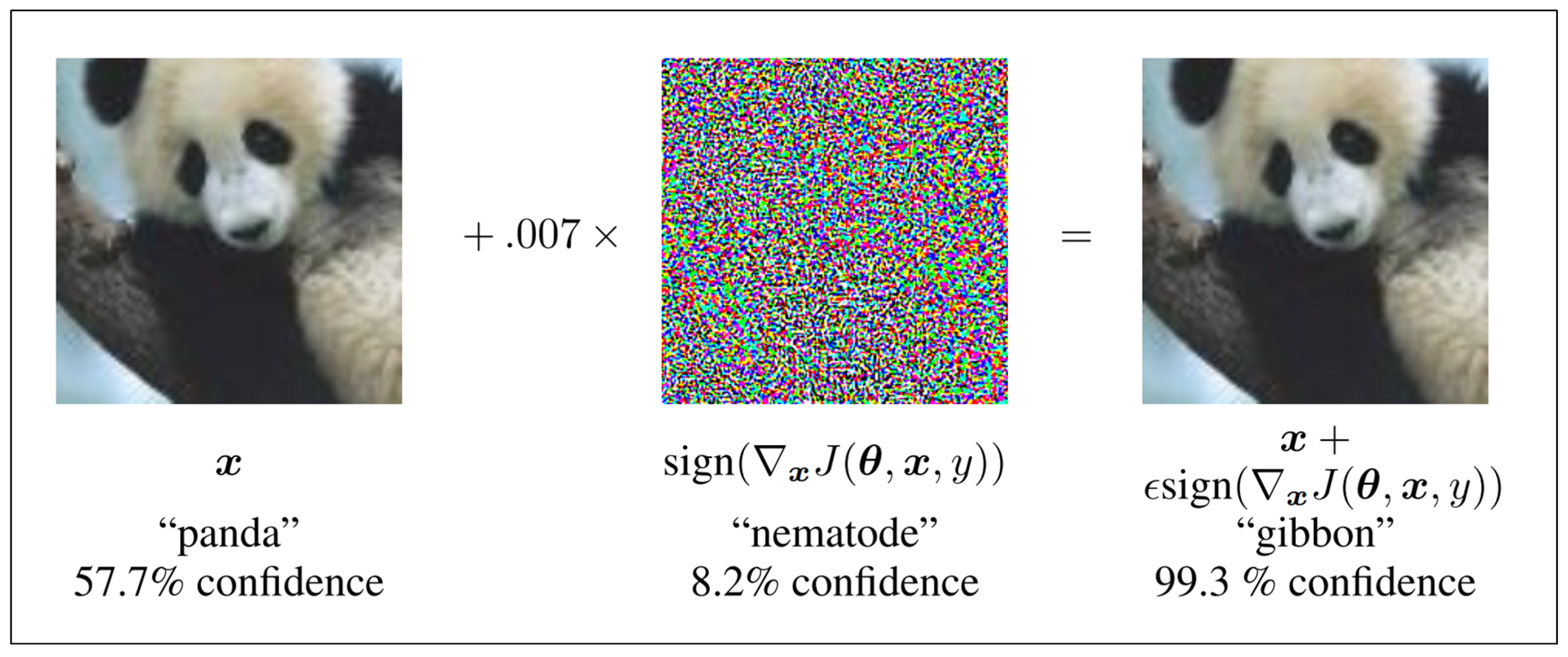
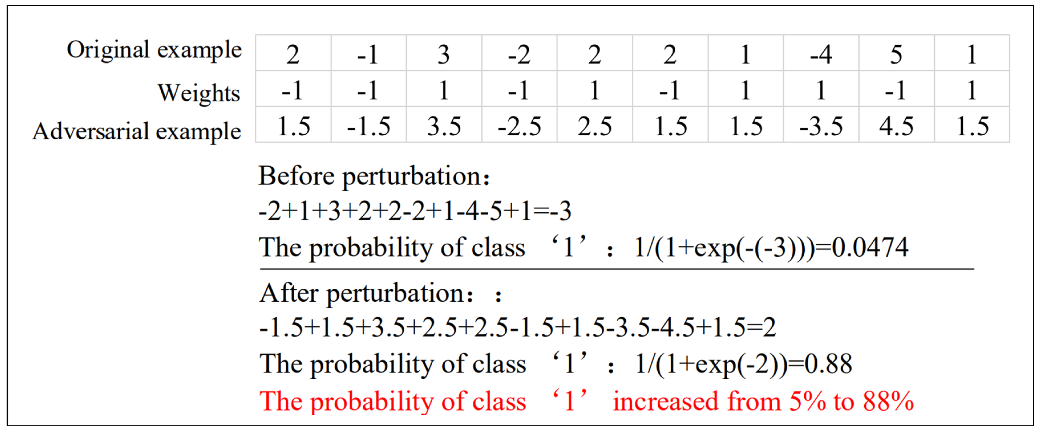
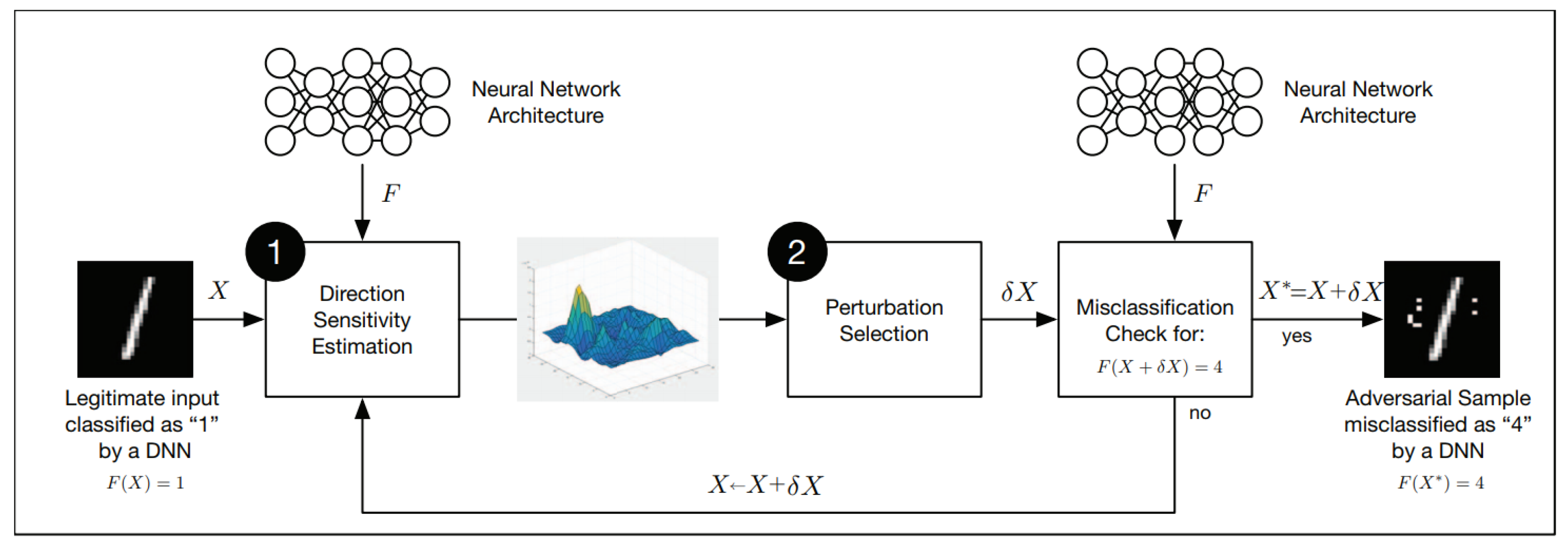
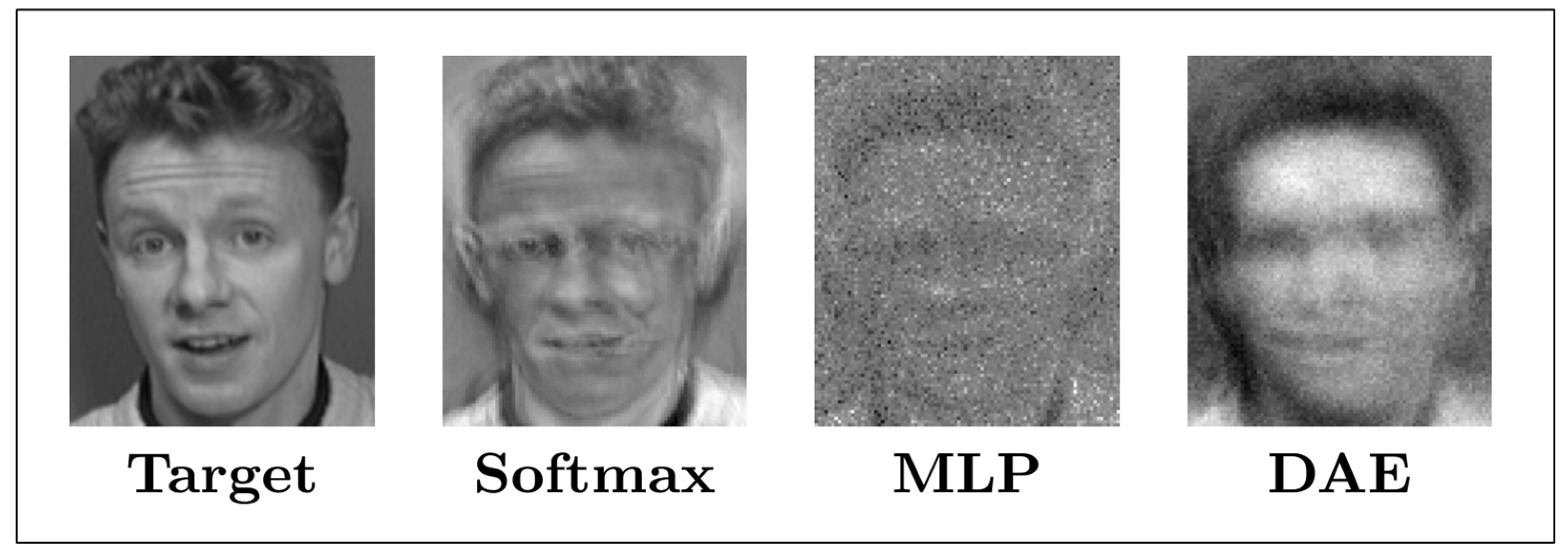
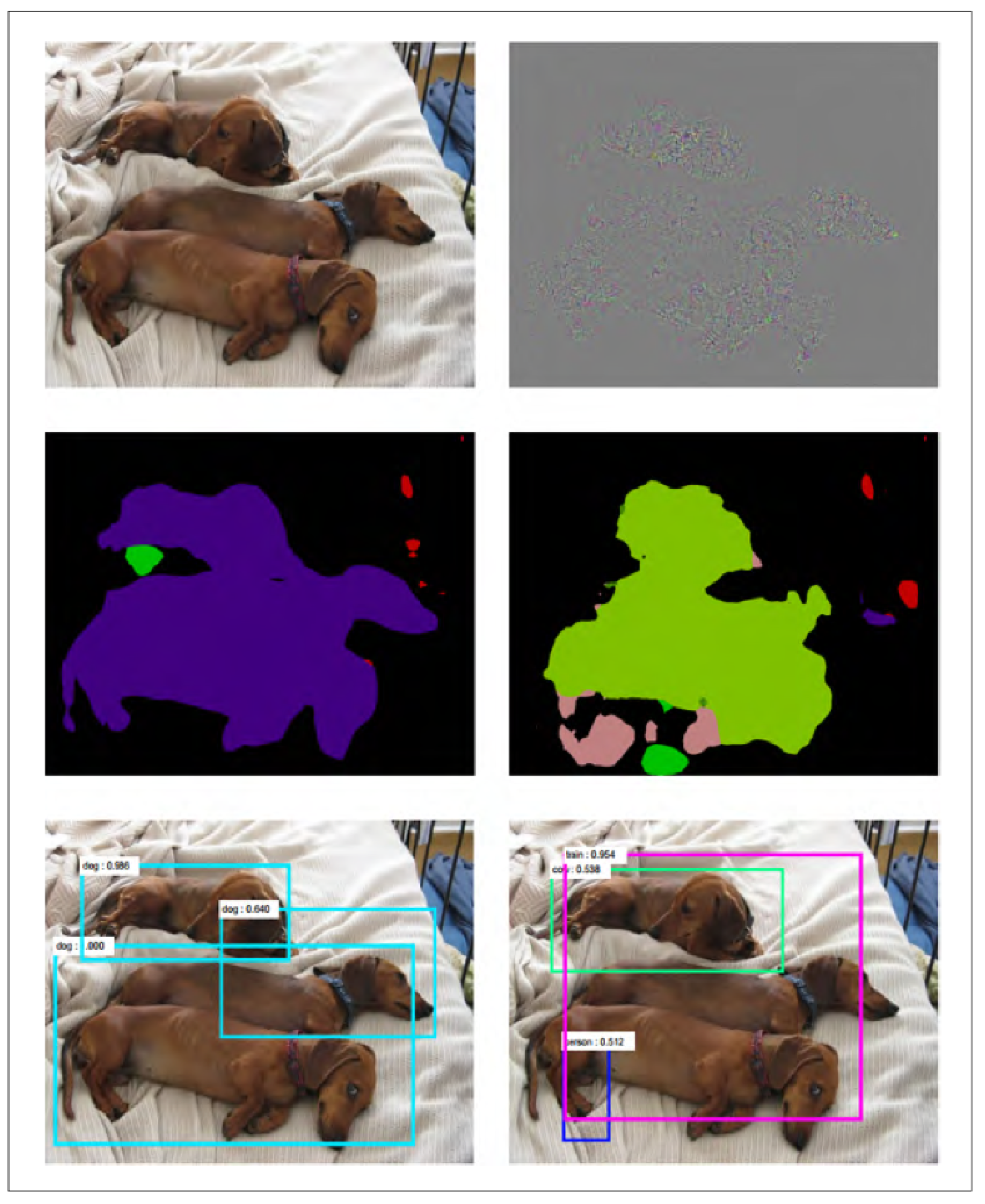
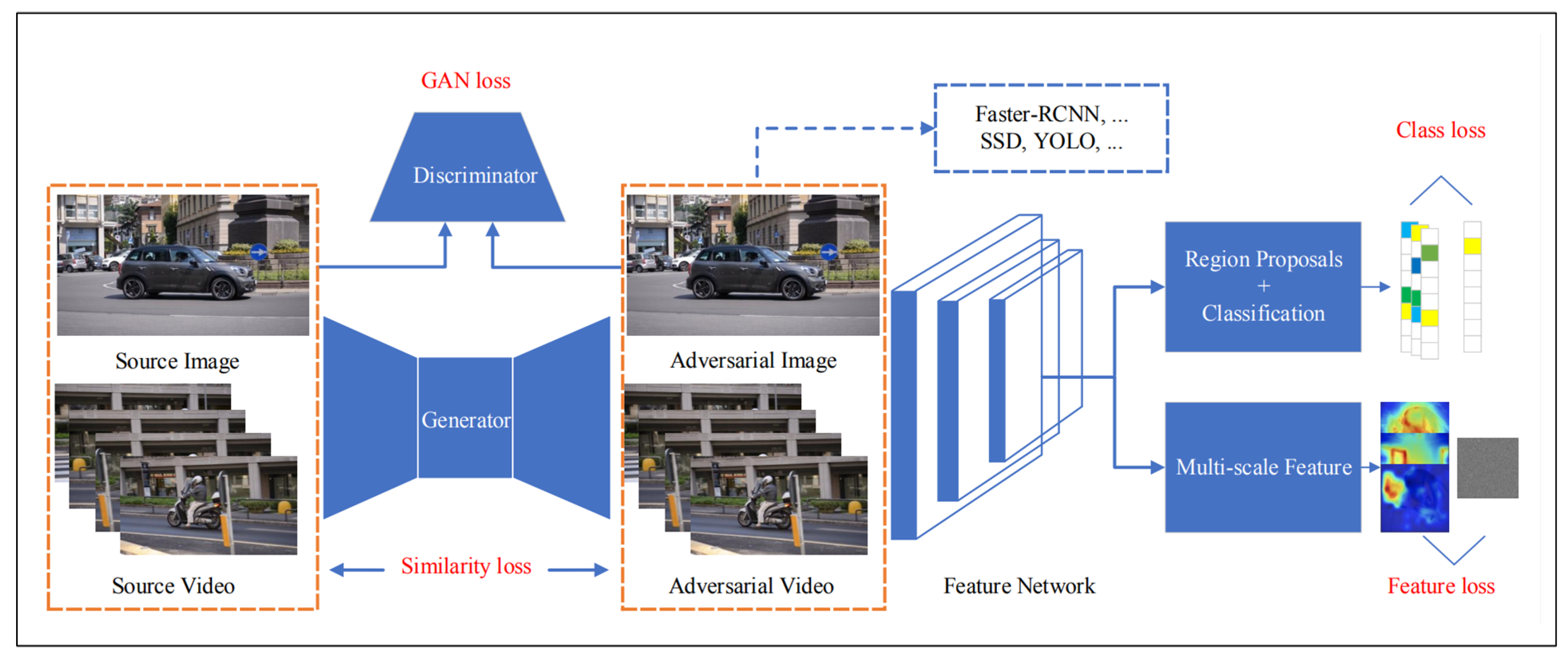
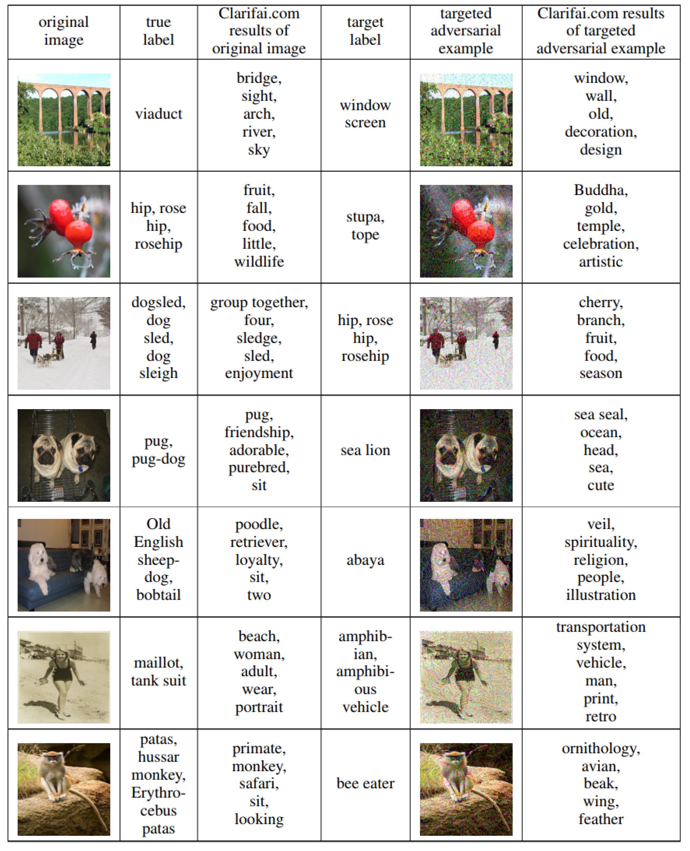
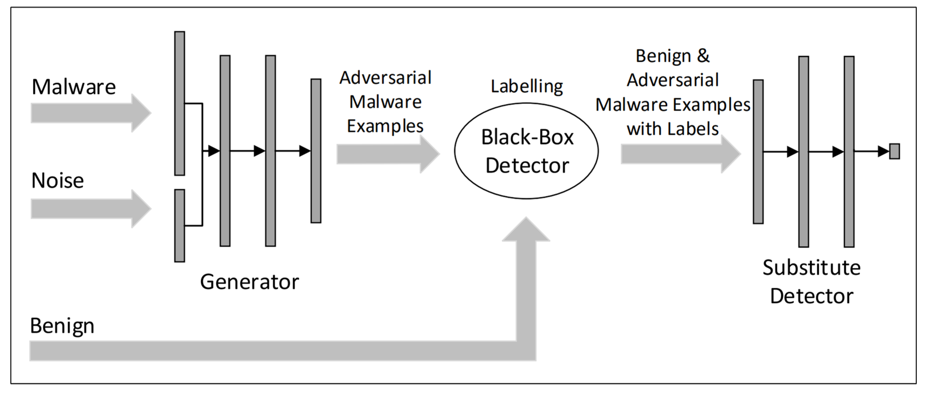
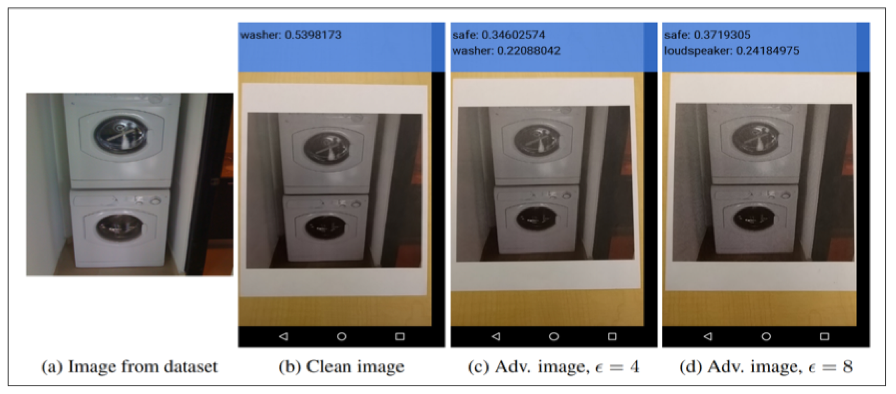
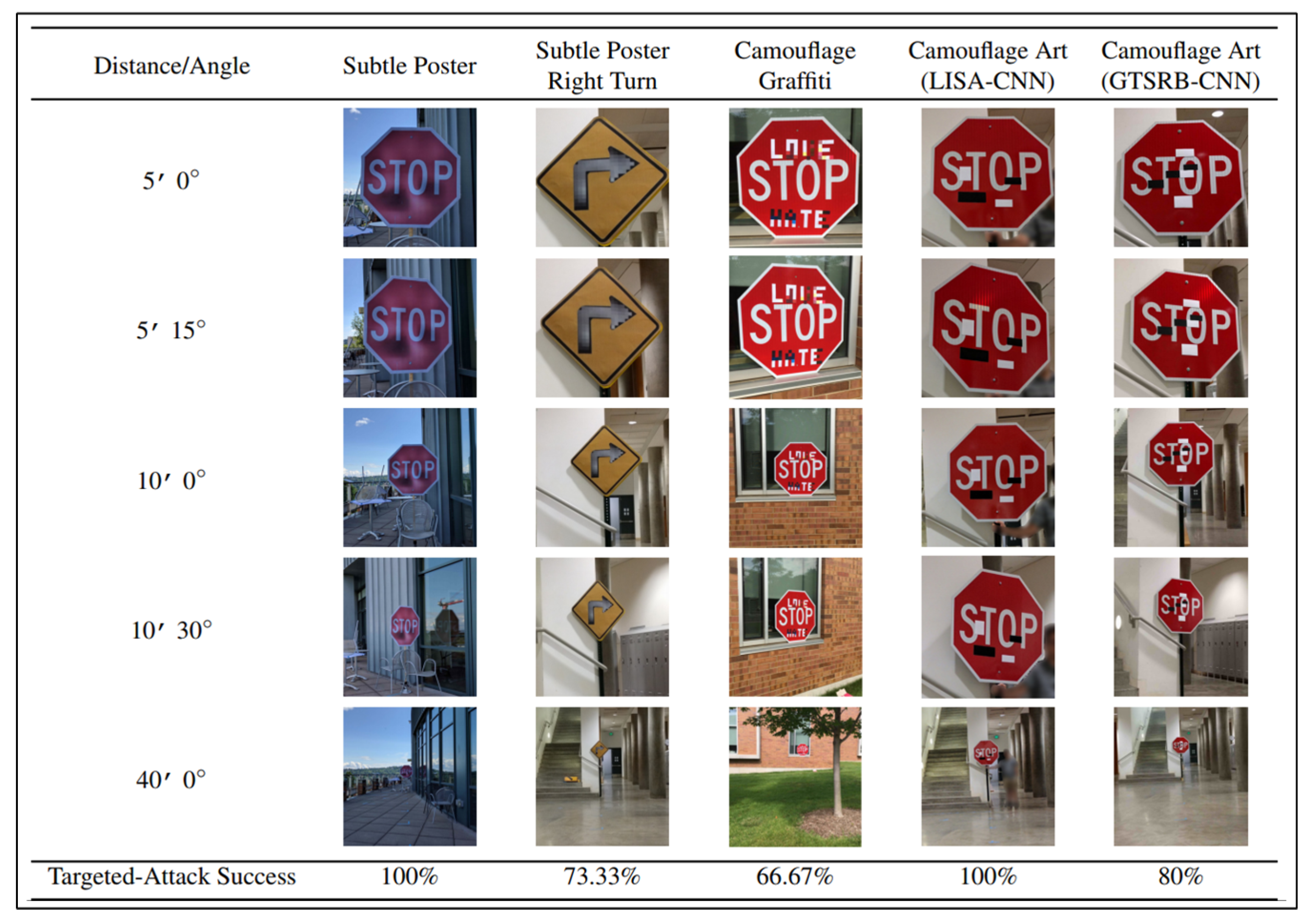
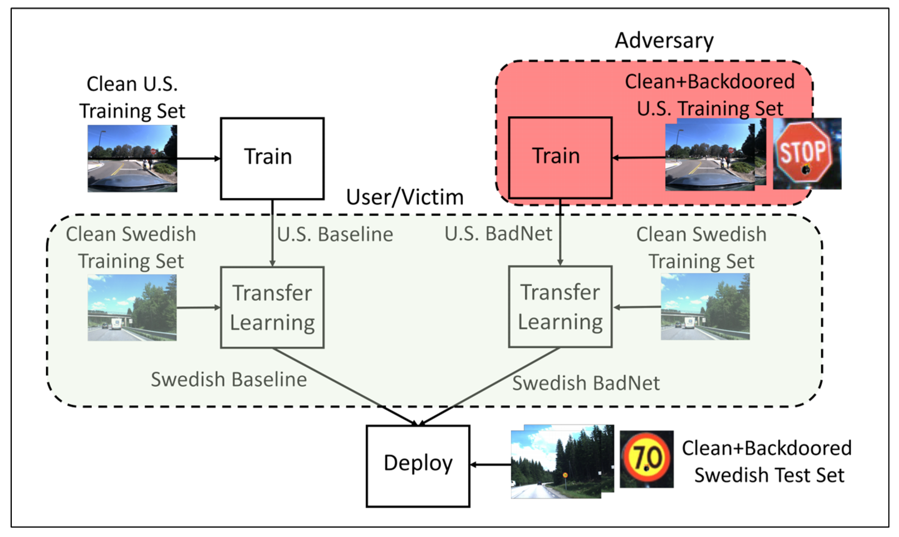
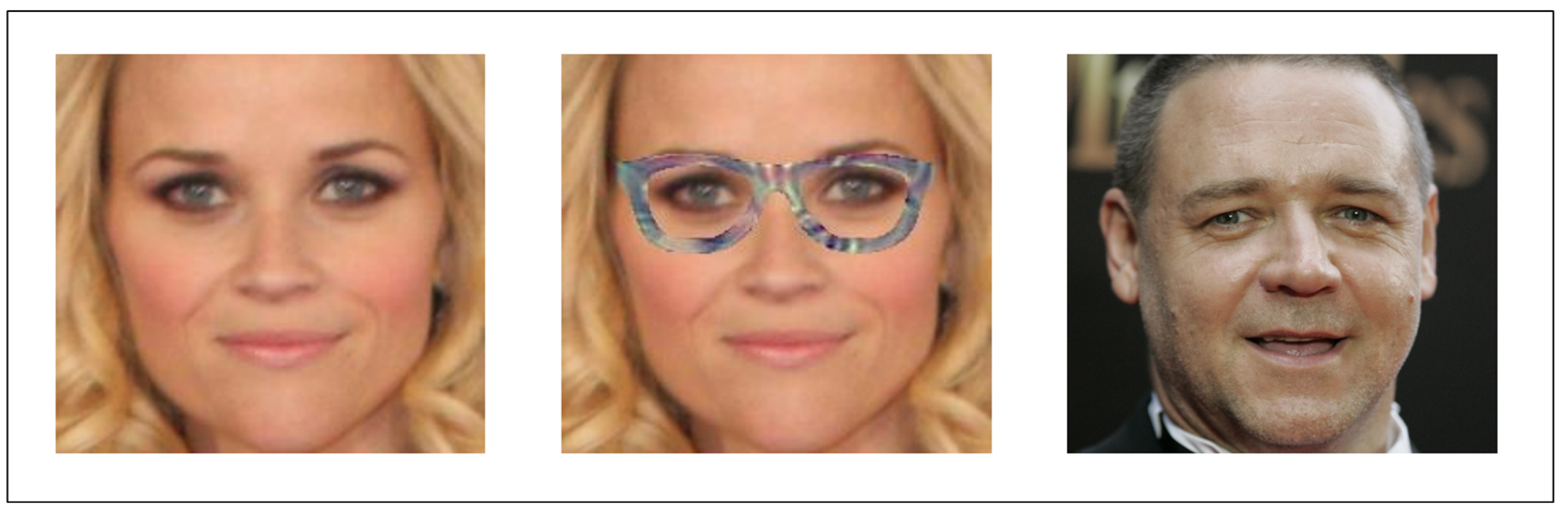
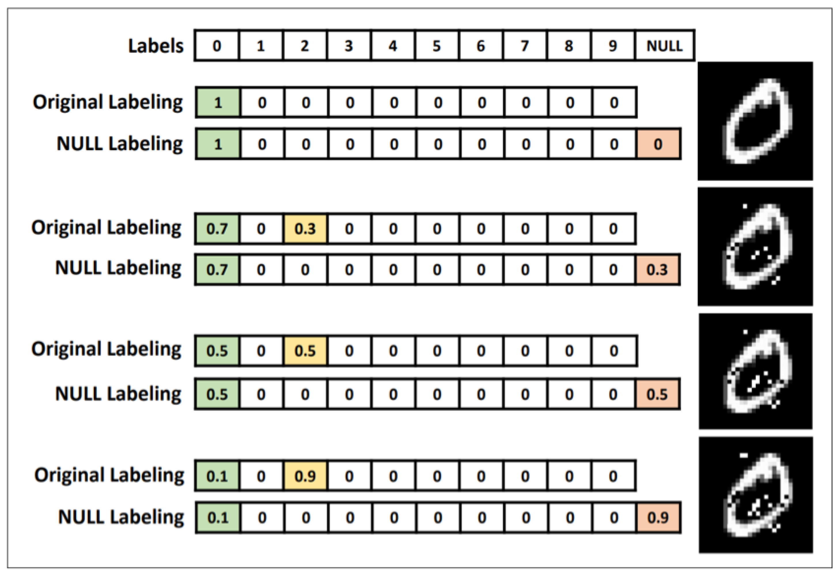
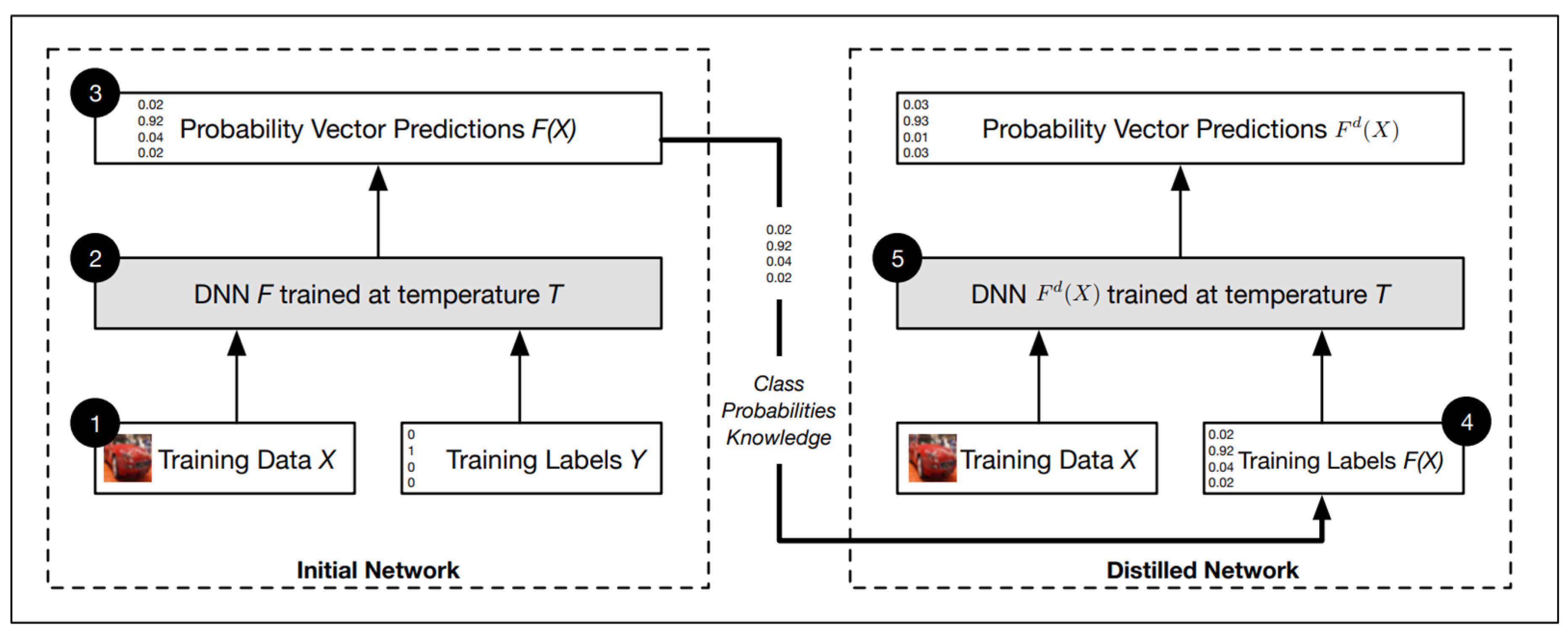
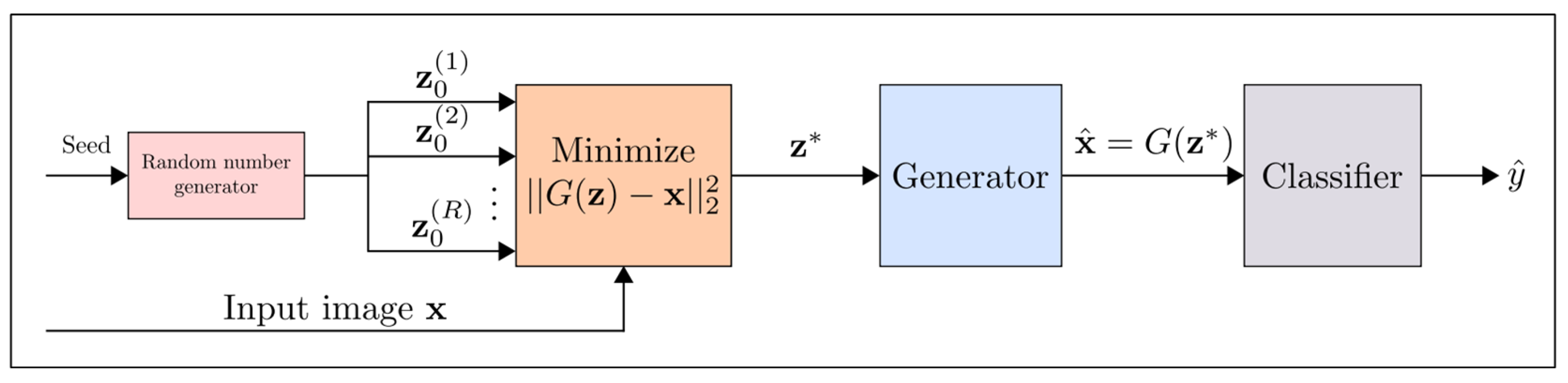
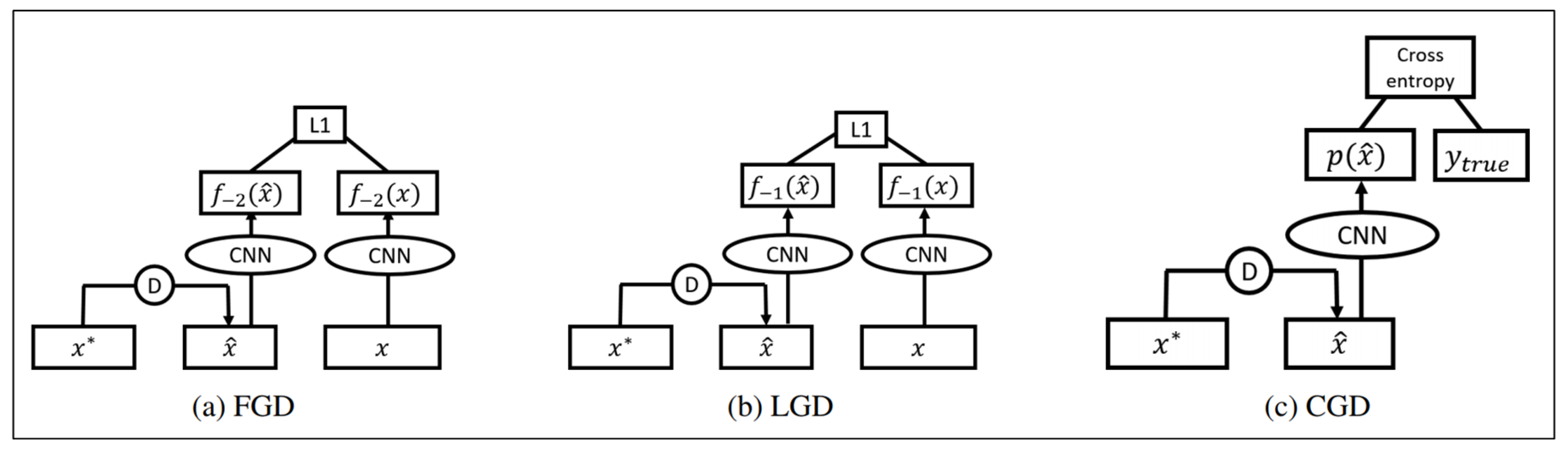
Table 1.
Applications of adversarial attack in image classification field.
| Articles | Methods | Main Ideas |
|---|---|---|
| Szegedy et al. [6] | L-BFGS | using L-BFGS algorithm to optimize the objective equation . |
| Goodfellow et al. [15] | FGSM | FGSM is used to calculate the gradient of the cost function relative to the input of the neural network, calculate Formula (4) to get adversarial samples and lead the target model to achieve 89.4% misclassification on the MNIST dataset. |
| Kurakin et al. [16] | One-Step Target Class | Calculating the Formula (5) to get adversarial samples. |
| Kurakin et al. [16] | BIM | The adversarial samples generated by FGSM are used in each iteration to generate final adversarial samples by small step length iteration. |
| Kurakin et al. [16] | ILCM | Replacing the target label in the BIM method with the most unlikely labels predicted by the classifier. |
| Papernot et al. [17] | JSMA | Directly providing the gradient of the output component to each input component, and the resulted knowledge is used in complex saliency map methods to generate adversarial samples. |
| Su et al. [18] | One Pixel | Only modifying one pixel per image to generate adversarial samples. |
| Carlini et al. [24] | Carlini & Wagner | Limiting the norm, norm and norm of the perturbations. |
| Moosavi-Dezfooli et al. [19] | DeepFool | Calculating the minimum norm adversarial perturbation iterative method. |
| Moosavi-Dezfooli et al. [64] | Universal perturbation | Generating image independent general adversarial perturbation for many different models. |
| Sarkar et al. [65] | UPSET | Universal Perturbations for Steering to Exact Targets (UPSET) introduced residual generation network, whose input is target class t and output is image unknown disturbance . |
| Sarkar et al. [65] | ANGRI | Antagonistic Network for Generating Rogue Images (ANGRI) calculated image detail perturbation in a closely related way. |
| Cisse et al. [20] | HOUDINI | Deceiving the gradient-based learning machine by generating adversarial samples that can be customized for task loss. |
| Baluja et al. [66] | ANTs | The Adversarial Transformation Networks (ATNs) used a feed-forward neural network to generate adversarial samples. |
| Chen et al. [25] | ZOO | Using the zero-order (ZOO) random coordinate descent method combined with dimensionality reduction, hierarchical attack, and importance sampling technique to carry out black-box attacks effectively. |
| Ilyas et al. [67] | variant of NES | The variant of Natural Evolution Strategies (NES) Proposing the adversarial sample generation method under query limit setting, partial information setting and label only setting respectively. |
| Li et al. [68] | Active learning | Using the white-box attack method to generate samples for queries, and introducing an active learning strategy to significantly reduce the number of queries required. |
| Adate et al. [69] | GAN-based | Using GAN to generate adversarial noise and classify the individual image. |
| Dong et al. [26] | Momentum | Proposing an iterative algorithm based on momentum to enhance the success rate of adversarial attack. |
© 2019 by the authors. Licensee MDPI, Basel, Switzerland. This article is an open access article distributed under the terms and conditions of the Creative Commons Attribution (CC BY) license (http://creativecommons.org/licenses/by/4.0/).
Share and Cite
MDPI and ACS Style
Qiu, S.; Liu, Q.; Zhou, S.; Wu, C. Review of Artificial Intelligence Adversarial Attack and Defense Technologies. Appl. Sci. 2019, 9, 909. https://0-doi-org.brum.beds.ac.uk/10.3390/app9050909
AMA Style
Qiu S, Liu Q, Zhou S, Wu C. Review of Artificial Intelligence Adversarial Attack and Defense Technologies. Applied Sciences. 2019; 9(5):909. https://0-doi-org.brum.beds.ac.uk/10.3390/app9050909
Chicago/Turabian StyleQiu, Shilin, Qihe Liu, Shijie Zhou, and Chunjiang Wu. 2019. "Review of Artificial Intelligence Adversarial Attack and Defense Technologies" Applied Sciences 9, no. 5: 909. https://0-doi-org.brum.beds.ac.uk/10.3390/app9050909
Note that from the first issue of 2016, this journal uses article numbers instead of page numbers. See further details here.