Reception of OAM Radio Waves Using Pseudo-Doppler Interpolation Techniques: A Frequency-Domain Approach

Canada Research Center, Huawei Technologies Canada Co. Ltd., 303 Terry Fox Drive, Kanata, ON K2K 3J1, Canada
Appl. Sci. 2019, 9(6), 1082; https://0-doi-org.brum.beds.ac.uk/10.3390/app9061082
Submission received: 31 January 2019
/
Revised: 7 March 2019
/
Accepted: 10 March 2019
/
Published: 14 March 2019
(This article belongs to the Special Issue Novel Insights into Orbital Angular Momentum Beams: From Fundamentals, Devices to Applications)
Abstract
:This paper presents a practical method of receiving waves having orbital angular momentum (OAM) in the far field of an antenna transmitting multiple OAM modes, each carrying a separate data stream at the same radio frequency (RF). The OAM modes are made to overlap by design of the transmitting antenna structure. They are simultaneously received at a known far-field distance using a minimum of two antennas separated by a short distance tangential to the OAM conical beams’ maxima and endowed with different pseudo-Doppler frequency shifts by a modulating arrangement that dynamically interpolates their phases between the two receiving antennas. Subsequently down-converted harmonics of the pseudo-Doppler shifted spectra are linearly combined by sets of weighting coefficients which effectively separate each OAM mode in the frequency domain, resulting in a higher signal-to-noise ratios (SNR) than possible using spatial-domain OAM reception techniques. Moreover, no more than two receiving antennas are necessary to separate any number of OAM modes in principle, unlike conventional MIMO (Multi-Input, Multi-Output) which requires at least K antennas to resolve K spatial modes.
1. Introduction
Since 1992, much effort has been devoted to the exploitation of the property of waves called orbital angular momentum (OAM). Although it appears to be newly-appropriated from the physics community, OAM has been known previously, especially in the RF (Radio Frequency) community, as phase modes. Phase modes were useful for synthesizing excitations of circular arrays in radio direction-finding and null-steering applications since the 1960’s [1,2,3,4]. Since the advent of multi-input multi-output (MIMO) technology in radio communications, OAM came to be recognized as another spatial dimension to be exploited for enhancing capacity of radio communications, and also optical communications in free space as well as fiber. An excellent historical summary of the development of OAM applications is given in [5].
No shortage of literature exists about how to generate and characterize OAM radio and optical waves [6]. Relatively few investigations focus on applications in radio communications, which is our interest in this paper, along the lines of [7,8].
Even fewer investigations focus on the receiving end of OAM communications links, with most of them relying on spatial techniques employing the same principles as those for generating the OAM modes at the transmitting end.
Consequently, most attempts at exploiting the OAM modes to enhance capacity of radio links suffer from the limitations imposed upon the receiver and antennas due to the spatial minima of all nonzero-order OAM modes’ beams on their axes, in the far field beyond the Rayleigh distance [7], where the receiver is situated. These limitations lead to low signal-to-noise ratios (SNRs), or very large receiving antennas, limitation to very short wavelengths, or limitations to short ranges comparable to the Rayleigh distance, or some combination of these. Additionally, real-world effects of antenna imperfections, multipath and dispersive propagation only add to the difficulties of reliably receiving and resolving the OAM modes and extracting the information streams from them.
Of all the more than 300 references cited in [6], only two [9,10] are about methods of reception and resolution of OAM modes that do not rely on variations of the spatial matched-filter concept whereby the helical phase fronts of the OAM beams are “untwisted” back to planar ones by the receiving antenna structure.
In this paper, a variation of the method of [10] is pursued to show mathematically, and via simulation, how it can be applied to the transmission and reception of multiple OAM modes simultaneously without incurring most of the limitations of prior methods cited above. A patent-pending apparatus for realizing this method at a radio receiver in real-time is also described, coupled with a signal-processing algorithm to resolve the different data streams carried on the OAM beams.
Section 2 presents the background and pseudo-Doppler principles behind the “virtual rotational antenna” of [10] and relates it to the context of radio beams possessing OAM. Transmission of OAM-bearing radio beams is also briefly reviewed. Section 3 presents the expression for the received OAM radio signals at the output of the pseudo-Doppler modulated antenna apparatus and relates its parameters to the physical geometry of the antennas and radio link. Section 4 describes the signal processing algorithm which processes the pseudo-Doppler aggregate signal to resolve the data streams carried on the individual OAM modes and examines some of its variants and limitations. It also contains preliminary simulation results to support the analyses. Conclusions and directions for future work are presented in Section 5. Select mathematical details are contained in the appendices.
2. Background and Pseudo-Doppler Principles
2.1. Real and Virtual Doppler Effect
Because most of the analyses involve circular geometry, it is useful to proceed in those terms. Accordingly, visualize an antenna element at position “n” on a circular locus having radius R as in Figure 1, with a plane wave incident on it from a point source “P” at distance L from the center of the circle, in the far field. At the antenna element the phase of the incident plane wave relative to that at the source is given by
Next, imagine that the antenna is moving along the circular locus with tangential velocity, v, in the direction of the colored arrow. With the radius remaining constant at R, this velocity involves only the change in azimuth angle θ with time, as v = Rdθ/dt. The corresponding change in phase at the antenna is derived by applying the chain rule as
where fDoppler = v/λ is recognized as the Doppler shift frequency due to the tangential motion at velocity v. This frequency is imposed upon the signal received at the antenna and if its angular position varies uniformly in time as θ(t), it results in a sinusoidal frequency modulation of the received signal with a deviation equal to fDoppler (when elevation angle is ϕ = π/2) and phase corresponding to the azimuth direction of arrival of the plane wave. This is a first hint that spatial information about a received signal can be determined in frequency domain. This phenomenon is sometimes used in radio azimuth direction-finding applications.
The motion of the antenna does not have to be real—it can be emulated using several antennas spaced at intervals of d around the circular locus and switching their outputs to the analysis receiver at intervals of τ = d/v. It then appears to the analysis receiver that it is sampling the output of one antenna moving around the locus with velocity v at intervals of τ, because it observes the same Doppler shift, which is actually a pseudo-Doppler shift as there is no real motion involved.
In the present application any actual motion of the source or the receiving antennas will be assumed to be 0, and the source of the OAM signals will be positioned at elevation angle ϕ = 0 to keep the analysis simple. The reference phase can be taken at the center of the circle in the far field by setting L = 0. The only relevant phase shifts will then be relative phases between two or more antenna elements on the same locus.
2.2. Application to OAM Radio Waves in the Far Field
It is instructive to review the salient features of radio waves possessing various orders of OAM, which will be denoted by integers ±k. Such radio waves are generated by imposing a phase shift of k2π radians for every revolution of the observation point around the beam axis, giving it a helical phase front. This is not to be confused with polarization, which can be of any type. In RF applications, this can be relatively easily achieved using a uniform circular array of K identical antenna elements, each one fed by a current that is shifted in phase from that of its neighbor (in one direction) by k2π/K radians and with the same amplitude. Negative phase shifts generate OAM modes with helical phase fronts winding in the opposite sense around the beam axis, up to order K/2-1.
A common method of creating multiple OAM beam excitations of the same circular array of antenna elements is to connect the K elements to the K output ports of a modified Butler matrix, and the K input ports of that Butler Matrix to K transmitters in the same RF band, with each modulated by a different stream of independent data symbols. The Butler matrix must be modified so as to possess one port which gives rise to a zero-th order OAM mode; otherwise the electrical phases at the elements do not progress through an integer number of cycles so the phase fronts would not form continuous spirals.
When plotted in three dimensions, the beam patterns appear conical for all non-zero orders of OAM, as depicted in Figure 2, where color was used to denote the electrical phase at a fixed time, modulo-2π radians.
It is instructive to note that the phase (color) patterns rotate around the beam axis at the RF rate in time, i.e., one revolution per cycle of the radio frequency. Therefore, k-phase fronts (of a given color) pass a point on the cone of the k-th OAM beam in the tangential direction, per period of the RF carrier wave. Equivalently, at any given point in time, an electrical phase gradient of k2π/(2πR) radians per meter exists along the circular locus (also the beam footprint) around the axis of the conical beam of the k-th OAM mode.
In Figure 2, the antenna elements in the x-y plane numbered K = 16 and were omnidirectional, with the beam axes being in the z (vertical) direction.
With the help of Figure 3, visualize the circular locus of the antenna element in Figure 1 as coinciding with the peak of a conical beam of OAM order k, whose source is a circular array in the far field on the z-axis.
Because the elevation angle of the source is now ϕ = 0, the only phase variation along the locus of the antenna element at a given point in time is due to that of the OAM beam. The shaded circle denotes the footprint area of the k-th OAM beam.
Taking the phase at the x-axis as the reference phase of the moving antenna element, its phase at position θn is therefore given simply by
at a given point in time. As the antenna moves around the circular locus in the x-y plane with uniform velocity v, its angular position changes linearly with time, consequently causing its electrical phase to vary linearly with time according to (3) as
This can be related to a kind of “transverse” Doppler frequency shift because with R being constant, (4) can be written also as
since, according to the discussion of Figure 1, it is clear that
Thus, it has been shown that a spatial-domain property of an OAM beam of order k, the phase gradient k/R, can be converted to a frequency-domain property, namely a kind of transverse or rotational Doppler shift fn,Doppler, through the motion of the antenna element receiving the OAM beam. Note that the effect is real in the physical sense [9]; the subscript “n” may be omitted as there is only the one moving antenna. Note also, that this transverse Doppler shift is directly proportional to the OAM order, k, and independent of RF carrier frequency.
Next, invoke the pseudo-Doppler technique whereby the motion of a single antenna from position #1 to position #2 is emulated by switching among several antennas, as outlined at the end of subsection A. Specifically, let the receiver employ two antennas separated by distance “d” tangentially to the footprint of the OAM beam, and instead of switching between their outputs, the receiver combines their outputs in time-varying proportions ranging from only output #1, to half of each output #1 and #2, to only output #2. This is in effect a form of gradual switching between the antennas, in one direction; it is assumed to be repeated periodically at some rate in accordance with the principles employed in [10].
To understand how such time-variant combining emulates a transverse Doppler shift in the received carrier frequency, Appendix A reviews the principle of the Doppler effect in simple contexts. With that in mind, it is relatively easy to derive the key relation between the phases of the OAM beam as received at the two antennas at a given time in Figure 4.
At a given point in time, the phase of the RF wave arriving in the form of OAM mode k at RX antenna #1 is ψ1 and at the same time the phase at RX antenna #2 is ψ2. Because the phase delay advances k multiples of 2π radians for one complete trip around the footprint, 2πR, at a given observation point in time, it advances by proportion kd/(2πR) for the portion of the footprint covered by the antenna separation “d”. The phases at the two RX antennas are therefore related as
Consequently, the signals at the inputs W1 and W2 of the time-varying combiner are modeled as being multiplied by the complex-exponential phase factors as
where Sk(t) is the signal of the k-th OAM beam received at the reference point in the far field.
Before exposing the function of the time-varying combiner in Section 3, the next subsection describes briefly the transmitting end of the link where the multiple OAM beams are modulated with independent data streams on the same RF carrier and launched from the antenna structure. In this respect, the multiplexing of several data streams onto several OAM beams is still effectively performed in the spatial domain as in all other OAM transmission schemes in RF applications.
2.3. Transmission of Multiple Overlapping OAM Radio Beams
In numerous past applications, the axial beam patterns of phase modes, or OAM modes in modern parlance, have been derived and characterized as being proportional to [4]
where Jk is a Bessel function of the first kind, order k, r is the radius of the circular antenna array, ϕ is the elevation angle measure from the beam axis and λ is the wavelength of the RF carrier wave of the k-th OAM mode. The first few orders of this Bessel function are shown plotted in Figure A3 of Appendix B.
Consequently, it is seen that OAM beams of higher orders have wider cone angles in the far field than those of lower orders, and beams of different OAM orders do not overlap much in space (except negative and positive modes of the same order). That is also evident from Figure 1, which was plotted in accordance with Equation (9) and Appendix B, where the peak positions along the x-axis correspond the peaks of the conical OAM beams at radii “R” from the beam axis. Clearly, the higher-order Bessel functions having peaks at larger values of “x” means that higher-order OAM modes have peaks at larger radii from the axis, hence larger cone angles, as dictated by (9). Also evident from (9) is the property that an OAM beam of order k generated from an array with a larger radius will have a smaller cone angle than the same OAM of order k generated by an array with a smaller radius.
Because it is desired to transmit multiple data streams on the same RF carrier to one user using multiple OAM beams, their conical beam patterns must overlap at the user’s location in the far field. Therefore, all OAM modes cannot be launched from the same circular array of antenna elements, but the lower-order ones should be launched from arrays having proportionally smaller radii and the higher-order ones from arrays having proportionally larger radii. These arrays may be concentrically stacked as shown for example in Figure 1a of [11], adapted below as Figure 5. Such a transmitting antenna arrangement is expected to be of the same physical size as in other, more “conventional” RF schemes for transmitting OAM beam and no attempt to improve the link SNR is inferred here; that is effected at the receiver—as will be shown in subsequent sections.
3. Real-Time Implementation of Pseudo-Doppler Effect on Received OAM Beams by Dynamic Antenna Combining
As noted in the Introduction, very few attempts at OAM multiplexing in electromagnetic-wave communication links did not rely on spatial rectification of the helical OAM phase fronts at the receiver, but a few should be mentioned before proceeding to describe the present scheme as being unique.
Reference [12] even uses a time-based method for generating OAM modes in circular arrays, which saves some hardware but otherwise is not really necessary for overcoming difficulties in implementing an OAM communications link. A simple phase-gradient measurement is used in [13] to sequentially detect OAM modes, which are sequentially encoded with data symbols at the transmitter. The authors of [14] also use the phase gradient to resolve the OAM modes at the receiver, by switching between multiple pairs of receiving antenna elements.
In [15], the authors use the phase gradient sensed by switching between two receiving elements to identify the transmitted OAM mode, which corresponds to an encoded data symbol. This generates harmonics of the switching frequency, which are used to detect the (sequentially) transmitted data symbol. No dynamic combining effects are employed, and the data symbols are transmitted and decoded sequentially.
Another variation of the time-gated generation and detection of OAM modes appears in [16], using strategically-placed antenna elements covering only part of the circular aperture that an array such as the one in [11] would utilize. The results appear rather stochastic, with relatively high cross-talk among the detected OAM modes.
A partial-circle aperture approach was also used by the authors of [17] to avoid the size issue with “conventional” OAM receiving antenna arrays. Judicious selection of the fraction of circle covered by the receiving array renders the received OAM modes orthogonal at the receive array, thus allowing them to be resolved and independently decoded. A variation on the time-switched array method of generating OAM modes using sinusoidal modulators instead of switches at the elements of a circular array is described in [18]. It is not applicable, nor easily convertible to receiving OAM modes.
In this work the driving interest is to explore ways of implementing the method advanced in [10] in real-time, to realize a more practical OAM receiver than has been possible using co-axial spatial receiving techniques based on circular antenna arrays.
In the process, it became evident that important details of the pseudo-Doppler technique are not derived with sufficient persuasion for this author, so another aim of this work is to fill in the mathematical details that allow an actual OAM radio communications link to be conceived and simulated.
Specifically, it was noted that an actual demonstration of a real-time pseudo-Doppler-shifted spectrum of the received OAM signal carrying a useful data rate was not documented in the relevant literature; in [9] the spectrum shifts shown were caused by real Doppler shift due to physical rotation of the antenna, and in [10] the spectra were obtained by off-line post-processing of rather narrow-band data. The supplementary material shows ideal sketches of the shifted spectra and also spectral shifts due to rotation of the transmitting antenna; actual demodulated data is not represented, as that was an aim of future research stated in [10].
3.1. Using a Quadrature RF Oscillator and Mixers
Without belaboring the details, a way of implementing the relative dynamic weighting of the two receiving antenna signals comes to mind using orthogonal sinusoidal modulations, visualized as in Figure 6. It is even simpler to implement than an image-rejecting mixer in the front end of many common microwave radio receivers. Note that the sinusoidal wave generator can have a very high rate, as microwave oscillators are very common and straight-forward to implement. (This high rate will be necessary to separate the OAM signals in frequency domain, thereby facilitating their signal recovery. A real Doppler shift of such a frequency would require physical motion at speeds approaching the speed of light.)
By strategically working through the mathematics of the output equation in Figure 6, the result for the output during selected time-gated intervals can be obtained approximately as
with the understanding that Ω = 2πF is the radian pseudo-Doppler frequency, F being the corresponding frequency in Hz. Note that the bottom factor is due purely to the effect of the pseudo-Doppler modulator on the OAM incident wave, and the scaled pseudo-Doppler radian frequency shift kΩd/(2R) is independent of the RF carrier radian frequency ω, which is implicit in S(t), which in turn is the transmitted signal on the k-th OAM mode,
with m(t) being the modulating signal and ω being the radian carrier frequency.
Before developing the models for the necessary time-gating and demodulation functions, it is instructive to estimate the potential performance of this method of OAM reception in terms of link and antenna geometry.
3.2. Implications in an OAM Radio Link
As pointed out in [10], the resulting scaled pseudo-Doppler shift at the output of the combiner in the front end of the receiver should be greater than the bandwidth, B, of the transmitted signal in any OAM mode (assuming each OAM mode carries an independent data stream at the same rate of B symbols/second). So one “unit” of frequency shift corresponds to k = 1 and satisfies
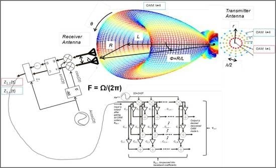
in keeping with radian units of frequency. In the example depicted in Figure 7, choose the parameters as in Table 1 below. The condition 0.02k = kd/(2R) << π/4 is satisfied.
From (22) and Table 1 the oscillator frequency for the pseudo-Doppler modulator of the receiver front end in Figure 7 is determined to be F = 2 GHz. This is a typical frequency in modern mobile radio hardware so the modulator and oscillator are easily achieved. The effective pseudo-Doppler shift of the k= 4 OAM mode will be 40 MHz.
Note that the receiving antenna array in Figure 7 is not positioned on the beam axis as in “conventional” RF links employing OAM beams, but at the peak of the OAM beams which is at a radius R perpendicular to the axis. It is this arrangement which enables a higher SNR at the receiving end, owing to the much higher OAM signal amplitude there.
Given the size of RF wavelengths, it would be grossly impractical to capture all of the OAM beam energy at radius R as the receive antenna array would need to be of the same order in size. As also stated in [10], it would be equally impractical to physically rotate such an antenna to impart a Doppler shift to its output, hence the motivation to use a virtually-moving, electronically interpolated antenna, to impart the much higher Doppler frequency shifts to the OAM modes using pseudo-Doppler techniques. It is not difficult to perceive that, despite having only two receiving antennas (necessarily) positioned off-axis, the SNR at the receiver can be much higher than that obtainable from a similar size of receiving radio antenna array necessarily positioned on-axis.
Therefore, the subsequent signal processing of the pseudo-Doppler shifted OAM beam signals in the frequency domain is expected to yield much “cleaner” recovered OAM signals, at longer link distances in free-space RF applications than a conventional spatial OAM recovery technique relying on the reciprocity of launching OAM modes with a similarly-sized antenna array. (Note that even in such reciprocity-based spatial OAM recovery schemes, the receiving antenna is not large enough to capture all of the beam energy contained in the toroidal “footprint” with radius R of the OAM beams at link distance L. The SNR penalty of those schemes is not due to the size of their receiving antennas so much as it is due to their necessary positioning on-axis, where all (non-zero-order) OAM modes have a deep amplitude minimum and are spatially orthogonal.) Further possibilities for enhancing the effective SNR by frequency-domain signal-processing are described in Section 4.3.
To determine the size of the transmitting antenna array, it is observed in Appendix B that the peak of the k-th order Bessel function in (9) occurs roughly where its argument is equal to k + 1 for orders below about 6. The receiver is situated off-axis, at the peak of the overlapping OAM beams. (The antennas are not drawn to the same scale as the beam pattern and link geometry.)
Therefore for OAM mode k = 1, the radius of the transmitting array is determined as
and for k = 4, the radius of the TX circular arrays is
Such size of antenna is not excessive for a sub-6 GHz base station. If the element spacing is to be half of the RF wavelength as indicated in Figure 7, then the outer array for OAM mode k = 4 would require 500 elements and the inner one for k = 1 would require 200 elements. Note that because negative OAM orders are equally handled by the same system (resulting in negative pseudo-Doppler shifts at the RX), a total of 9 OAM modes could be transmitted on this link.
4. Time Gating and Demodulation Algorithms
As noted in the discussion that relates Equation (10) to the output equation in Figure 6, the relevant approximations can be made only for certain periodic windows in time. Accordingly, the output signal at Z1 must be gated to be observable only at those times and suppressed at all other times. It amounts to imposing time-limited frequency shift on the received signals, the frequency shifts being the pseudo-Doppler shifts of the individual superposed OAM modes. This is recognized as the frequency-domain dual of the band-limited time-delay problem, the time-delay being a fraction of the sampling interval of a discrete-time signal [19].
4.1. Time GatingTo Emulate Motion of Antenna in One Direction
The limits of the region of validity of the pseudo-Doppler frequency shift as expressed in the output by (10) are actually periodic when the fundamental period being
in terms of phase. The output of the modulator summing junction in Figure 6, especially the bottom factor in Equation (10), must therefore be gated periodically in real time to ensure the desired frequency shifts in the final output. This periodic gating must evidently be synchronous with the pseudo-Doppler modulation, as (13) must hold for every period, or periodic values of nπ.
It is instructive to visualize this synchronous gating in relation to the modulations. When superposed on the effective sinusoidal modulation waveforms applied to the antenna output signals, cos(Ωt) to W1 and −sin(Ωt) to W2, the gating intervals are seen to contain those portions of the modulations which cause one antenna output to be increasing and the other decreasing the magnitude of its contribution to the output. The alternating signs of the gating waveform based on (13) ensure that the same antenna output is always increasing while the other is decreasing. This shows that the apparatus performs the desired interpolation that emulates a moving antenna between the two stationary receive-antennas as described in [10]. Figure 8 illustrates the periodic gating of the modulation waveforms.
The gating windows are denoted by the values of the period “n”, and their multiplier signs by their positions either above (“+”) or below (“−”) the angle (“normalized time”) axis. Note that the angle axis is calibrated in multiples of π/4 radians.
4.2. Simulation of Basic Pseudo-Doppler Modulator and Gating Arrangement
A preliminary numerical simulation to verify the proposed concept was conducted using MATLAB® R2012a (7.14.0.739) and Simulink® R2012a (7.9), with Communications System Toolbox (5.2), DSP System Toolbox (9.3) and Signal Processing Toolbox (6.17).
For reference, the transmitted constellation from one of the sources is observed via a matched pulse-shaping filter, as shown in Figure 9a. Its spectrum is also observed; in fact, the spectra of all the sources are the same on average and are shown in Figure 9b as seen when superposed at one receive antenna (They would appear the same on average at the other receive antenna.)
So, all the OAM modes (OAM 1 and OAM 8 in this case) occupy the same spectrum shown in Figure 9b, which is the only spectrum visible in the transmission medium and potentially subject to regulation. Yet, it will be shown that the OAM modes can be recovered separately from this composite signal in the receiver.
After modulation by the pseudo-Doppler waveforms, time-gating and down-conversion, the constellation and spectrum of the composite received signal appears as in Figure 10a,b respectively. The down-conversion frequency is 0 Hz in this case, but in general it will be some multiple of 2F, where F is the pseudo-Doppler modulation frequency, because the gating pulses occur 2 times per cycle of F and they have harmonics.
Note that the spectrum of the receiver output composite signal consists of many harmonics of twice the pseudo-Doppler modulating frequency imposed at the receiver front end and is generally not symmetric about 0 Hz. Also note that the constellation does not look recoverable. The constellation is always obtained from the spectral replica positioned at 0 Hz after the down-converter.
It is interesting to observe the received constellation and spectrum of each OAM mode separately. This is shown, still with 0 Hz frequency shift in the down-converter, in Figure 11 below.
Note that, with a frequency shift of 0 Hz in the down-converter, OAM8 dominates over OAM1. With suitable scaling by a complex coefficient (amplitude and phase change), OAM8 could be recovered even in the presence of OAM 1, and after suitable conventional equalization and decoding, its QAM data symbols successfully demodulated.
With a different frequency shift applied at the down-converter, other OAM modes can be recovered. For example, it turns out in this case that with a shift of 2F, i.e., twice the pseudo-Doppler modulation frequency, the complementary situation arises, as shown in Figure 12.
Now with frequency shift of 2F in the down-converter, OAM1 dominates over OAM8, so OAM1 could be similarly recovered and demodulated in the presence of OAM8. Without any other signal processing, each OAM mode was recovered from the composite signal with an uncoded error rate in the order of BER ≈ 10−1. These examples were chosen because the differences in OAM proportions happen to be very obvious, but this is not always the case. Moreover, the expected spectral shifts by fractions of the pseudo-Doppler modulation frequency appear to be absent in all of the output spectra.
Were the above simulation results a lucky coincidence and did they disprove the theory of the pseudo-Doppler frequency shifting of the OAM modes? It will be shown in the next subsection that this is not the case. There it is made clear that these results inspire a recovery algorithm for all the superposed OAM modes, and their spectral shifts will be shown to exist in the envelopes of the spectra. The differences in OAM proportions (more precisely, linear combinations) in the spectral replicas can be algebraically inverted so as to isolate them in final recovery outputs of a signal-processing subsystem. Such a subsystem would be based on least-mean-squares (LMS) optimization techniques and can be made adaptive to optimize their recovery in some statistical sense, much like existing MIMO receivers or adaptive-array systems.
4.3. OAM Recovery Algorithm
As evident from the above simulation experiments, the OAM signals are present in different proportions in the various harmonic spectral replicas (more accurately, “spectral shifts”) of the composite received signal at the output of the gating subsystem. It is expected, and will indeed be shown, that these proportions are not random but fixed and deterministic, as are the relative amplitudes of the spectral replicas themselves (e.g., ranging from −60 to −90 dB in Figure 10). They are in fact determined by the physical parameters of the link, which can be made known to the receiver à-priori, thus enabling it to recover the OAM modes more effectively than was done in the simulation experiment. Specifically, several shifted spectra can be shifted to baseband and linearly combined so as to cause the amplitudes of the desired OAM mode to add and those of the undesired OAM modes to cancel coherently, using an LMS adaptive FIR (Finite Impulse Response) filter type of algorithm for each OAM mode. Subsequently, or as part of the LMS algorithm, the desired OAM mode is adjusted in amplitude and phase so its dynamic range matches that of the decision or demodulating subsystem, compensating for the dynamic range of the wireless link.
It is essential to recognize that the gating pseudo-Doppler modulations of the composite received signal constitute a “time-limited fractional frequency shift” operation on it in the discrete frequency domain. This can subsequently be recognized as the dual of a “frequency-limited fractional time shift”, or band-limited fractional delay operation on a signal in discrete time domain as detailed in [19]. Specifically, the gating frequency, (which is twice the pseudo-Doppler modulation frequency), 2F, and the fraction thereof comprising the OAM spectral shift, kd/(2R)F as evident in (10), correspond to the sampling interval and fraction thereof, respectively, in the band-limited fractional-delay problem treated in [19]. This can be expected on the basis of the duality relations that exist between time and frequency domains due to properties of the Fourier transform and its inverse that relates them. The property that sampling in time-domain at intervals T causes periodic extensions in frequency-domain by 1/T also helps to explain the received spectra observed in the simulations.
Appendix C derives the frequency-domain effect of the time-limited fractional frequency-shift and its direct implementation along the same lines of reasoning as [19] for the impulse response and direct implementation of band-limited fractional delay in the time domain. The former can then be applied to (10) to plot the envelope of its spectrum and reveal the fractional pseudo-Doppler frequency shifts of the OAM modes. It also serves as the basis for an algorithm to recover the individual OAM modes from the gated output of the pseudo-Doppler modulator, as will be shown in the sequel.
In order to discern the spectral shift by the fractional pseudo-Doppler frequency, the Fourier transform of (10) is derived, in stages. First, (10) is affected by the time-gating and frequency-shift function so it is rewritten as a product of the cosine-modulated signal and the gating function with frequency-shift, inside the Fourier integral as
where ψ1(t) = 0, ψk = (1 − π/4)kd/(2R) were substituted. The time-gating function with frequency-shift, based on (13) is deduced to be the convolution
The reasoning is that the gating function is a series of complex-valued pulses “shaped” as uk(t), repeating at intervals of π in Ωt (which is 1/(2F) in t), hence the convolution of uk(t) with the train of Dirac deltas. It is reasoned that the fractional pseudo-Doppler shift occurs only during the gating times, so those functions are coupled in the product. The additional feature is that the deltas alternate in sign. That feature may be absorbed by defining gk(t) as a product of the periodic extension of uk(t) with a square wave having period 1/F as in the simulation, where the phase-shift of π/4 centers the peaks in the gating intervals.
and rewriting (15) more “cleanly” as
with some foresight to the next stage of the derivation. That foresight is, that the above convolution has the Fourier transform Gk(f) given by
where use was made of some identities involving Poisson sums, as explained in Appendix D, and Π(f) is the Fourier transform of Π(t). Before proceeding to evaluate (18), it is useful for later stages of this derivation, to express the integrand in (14) as the product of the transmitted signal Sk(t) and the rest of the time function, calling it the pseudo-Doppler modulating receiver function hk(t), defined with the help of (17) as
Now the gated output spectrum denoted by (14) can be expressed as the frequency-domain convolution of two Fourier transforms, namely (19) above convolved with Sk(f), which is the Fourier transform of Sk(t) and 2πF = Ω as usual. Therefore, the gated output spectrum (14) can now be expressed as the convolution of (18) and (129):
A further simplification is afforded by combining the cosine in (19) with the sine in (16), reasoning that (16) can be adequately represented by its fundamental-frequency component and the signum function dispensed with, so (19) becomes
Using a trigonometric identity for the top line of (21) with a/2 = 2πFt and b/2 = π/4 in
simplifies it to
Now, with the help of (23), the final output spectrum (30) can be expressed as
with the understanding that
This means that the spectrum of the gated output is a periodic extension of the transmitted spectrum of the signal with repetition interval equal to twice the pseudo-Doppler modulation frequency, 2F, multiplied by the spectral envelope Uk(f).
The next step is to evaluate Uk(f), which is the envelope of the spectrum, and manifests the fractional pseudo-Doppler frequency shift expected according to the order, k, of the OAM mode. This shift is traceable to the complex “pulse shape” function uk(t) defined in (15). Then the convolution with (25) is performed at the end. The spectrum of the envelope is
where the fractional pseudo-Doppler shift is
μk = F(kd/(2R)) in accordance with Appendix C. It is straight-forward but tedious to evaluate, producing
Then according to (24), the convolution of (27) with (25) gives the complete spectral envelope
Therefore, a sufficiently representative expression for the final output spectrum can be obtained by using (28) in (24) to obtain the output spectrum
It remains to evaluate (28) and plot its amplitude, so as to visualize the fractional pseudo-Doppler frequency shift at the output of this receiving subsystem.
The magnitude of (28) is plotted in the subsequent Figure for the parameters used in the simulation with k = 8 in
μk = F(kd/(2R)). What is actually plotted is the amplitude
with the common factor
being omitted for clarity. The spectral replica according to (29) are superposed at intervals of 2F.
Equation (29) is representative of the final output of the gating subsystem of the pseudo-Doppler modulated OAM receiver. Clearly, the spectral replica are spaced at twice the pseudo-Doppler frequency, 2F, while the peak of the envelope is at the fractional pseudo-Doppler frequency, μk = F(kd/(2R)), as expected and as observed in the simulation results. More accurate representation of the spectral envelope can be obtained by including higher harmonics of F when simplifying (16).
Now that it has been established that the gated output (29) consists of different proportions of spectral replica of each OAM mode, an algorithm for recovering them may be proposed. First it will be necessary to truncate the series of spectral replicas to a minimum equal to the number of OAM modes to be recovered, because at least that many different linear combinations of them will be needed. Each linear combination of spectral replicas is determined by the spectral envelope with its unique fractional pseudo-Doppler shift as in Figure 13. An arrangement such as in Figure A6 can be used to combine all the replicas in such a way that only those of the desired OAM mode will add up to a non-zero complex amplitude while those of all other OAM modes will cancel to zero, much like in adaptive-array signal-processing which nulls interfering sources’ signals. The coefficients should be low-pass so only the baseband spectral replicas are passed, as in down-conversion.
The OAM recovery process can be understood in terms of using (29) truncated to M = K terms and transformed into time-domain, as x(t) in (A14), where K is at least the number of OAM modes. The coefficients of the down-converted signals at each stage will be different than in (A14); they will now be derived jointly for all K of the OAM modes. Note that each stage has as input to its coefficient one of the spectral replicas (index “m” in (29)) of all the OAM modes superposed with their amplitudes as received upon. The stage inputs to the coefficients can be arranged in an Mx1 vector whose m-th row entry is
and Uk,m is the spectral envelope coefficient for the k-th OAM mode at the m-th spectral replica (i.e., stage coefficient). The lowpass signal at each stage is the same (because the spectral replicas are in fact replicas of the same signal, composed of all the OAM modes in their arrival proportions {ak}) so in vector-matrix form, (32) can be written as
where the time arguments were omitted for clarity. Further compacting the notation, one can write (33) as
where the matrix dimensions are shown explicitly to help with the defining correspondence with (33), with M ≥ K.
In order to recover all K of the OAM modes jointly, one needs K branches of the kind shown in Figure A6, each with M coefficients. That amounts to a KxM coefficient matrix C, which is derived next. When vector X is pre-multiplied by C, it will produce an output vector Y whose entries are the separated OAM mode signals. In fact, the OAM modes are present in their arrival proportions (which is understandable because the algorithm has no information about their transmitted proportions), so they will need to be equalized before they can be demodulated in the “conventional” way. The output vector is written as
By inspection of (34), it looks like the RHS of (35) may be obtained by pre-multiplying vector X by the inverse of matrix U. However, matrix U is not always square (unless M = K), so its inverse does not exist. Fortunately, the dimensions of the matrices and vectors involved are such that a pseudo-inverse does exist, which then becomes the desired coefficient matrix by correspondence with (35) as follows: Pre-multiply both sides of (34) by the Hermitian (complex-conjugate transpose) of matrix U, denoted as UH to obtain
Now notice that UHU is a K×K square matrix, so it can be invertible and one can pre-multiply both sides of (36) by it.
Denoting the pseudo-inverse of matrix U, which is found on the LHS of (37), as U# i.e.,
allows one to write (37) as is commonly done in least-squares optimization problems
so by correspondence with (35), the joint OAM recovery coefficients matrix is
Therefore, the recovered OAM modes are obtained from the input vector X simply as
which can be subsequently equalized and demodulated as in the “back end” (or DSP baseband section) of a “conventional” MIMO digital radio receiver. Although the matrix inverse found within the pseudo-inverse in (38) is not guaranteed to exist, it is more likely the more spectral replica are included, i.e., the larger the M is. It is dependent on the differences among the spectral envelopes of each of the OAM modes, which become more apparent as more spectral replica are included with increasing M. Increasing M beyond K does not increase the dimensions of UHU, but can improve its condition number, thus enhancing its invertibility. In other words, including more spectral components beyond the minimum number “K” can lead to better least-squares estimates of the OAM signals, with smaller error-vector magnitudes (EVMs) due to crosstalk.
Note also that this OAM recovery algorithm is deterministic because all the information contained in matrix U is known at the receiver, in principle. (The distance R from the beam axis may be deduced in non-fixed link via other signaling information such as timing-advance in TDD systems and from the TX antenna array geometry.) In practice U could be obtained by measuring the spectral-envelope coefficients of each OAM mode using correlation techniques during periodic “calibration” intervals, when each OAM mode would be transmitted separately. The coefficients for each branch according to (40) are shown explicitly in a sketch of the recovery algorithm in Figure 14 below (based on Figure A6 on Appendix C).
With suitable training signals for reference, an LMS type of algorithm can be formulated using well-known feedback loops to adapt the coefficients in the FIR-type of filter structure, as mentioned earlier. Moreover, including more than K spectral components and corresponding coefficient loops would provide more degrees of freedom, which could lead to further improved EVMs and potentially cancel external interference.
The structure in Figure 14 is reminiscent of a spectral-analysis process, so it may be feasible to implement equivalent versions of it using Fourier transform techniques. An acousto-optic spectrum-analyzer configuration comes to mind and may be pursued in future work.
It is also possible to make use of output Z2, noting that the output at Z2 can be derived by the same process as was that at Z1 but starting with
One obtains the corresponding result for Z2 prior to the gating operation, as
which looks like π/4 was replaced by −π/4 in Z1,k(t). Although one can make (10) and (43) look like the input by substituting cos(Ωt − π/4) = cos(Ωt + π/4 − π/2) = sin(Ωt + π/4) in (43), the change from π/4 to −π/4 also forces a change in the gating intervals. Using the same procedure as in Appendix D, it is found that (43) needs to be gated to intervals where
also separated by multiples of π, which are exactly complementary to those shown in Figure 8. That means the useful outputs at Z1 and Z2 after their respective gating operations appear in disjoint time intervals, so it makes no sense to combine them even though they have the same fractional pseudo-Doppler shifts that are desired. What does make sense is to “toggle” them to the same final output in order to have a more time-continuous output signal for the OAM recovery algorithm leading to (41), which may become useful in future refinements.
5. Conclusions
In this paper, a technique for recovering signals from received OAM beams based on pseudo-Doppler effect in the frequency domain was developed. Whereas reference [10] developed a method for detecting individual OAM modes based on an interpolation technique involving a minimum of two receiving antennas positioned tangentially on the peak region of OAM beams in the far field, this paper advanced the method to the point of recovering information carried on multiple OAM beams simultaneously, amenable to real-time implementation. Preliminary simulation results confirmed the ability of this technique to recover the modulation signals from several OAM beams in accordance with the mathematical least-squares type of signal-processing carried out in the frequency domain, based on the effect that the pseudo-Doppler technique imparts a different fractional pseudo-Doppler frequency shift to each received OAM mode. This technique was motivated by the observations that current spatial techniques for receiving and recovering the OAM modes in unguided radio-frequency applications are limited by the conical shapes of the (non-zero-order) OAM beams, which result in poor SNR, impractically large receiving antennas, short link distances, applicability to only very short wavelengths or guided propagation, or a combination thereof. These limitations are a consequence of attempting to receive and recover the OAM modes by the reverse of the spatial technique of transmitting them using co-axially situated circular antennas, motivated by increasing spectral efficiency of wireless links via spatial multiplexing. Here the spatial multiplexing applies at the transmitter, but the receiving technique essentially transforms the recovery problem into the frequency domain inside the receiver, keeping the radiated bandwidth the same. Other efforts at increasing data throughput of wireless links are directed at exploiting wide spectral bandwidth where available, using ultra wide-band (UWB) techniques, specifically UWB antennas [20]. Such efforts could be combined with the present OAM technique to further increase transmission capacity in the future.
Funding
This research received no external funding.
Acknowledgments
The author wishes to thank Huawei Canada R&D Center, Ottawa, for the support of this work-in-progress.
Conflicts of Interest
The authors declare no conflicts of interest.
Appendix A. The Doppler Shift
For completeness, the shift in the frequency of a propagating wave due to relative motion between source and receiver is reviewed.
Consider a stationary point at x = 0 with a wave incident on it at its propagation velocity, c, along the direction of the x-axis. Define the phase of the wave to be 0 there. With the help of Figure A1, the phase of any other point x(t) along the x-axis at the same instant in time is given by
Next, let the point x(t) move along the x-axis at a constant velocity v. Because the phase is linear with position, this will cause a corresponding linear change in its phase as it moves, given by
Figure A1.
Derivation of axial Doppler shift.

The rate of change of phase with respect to time is defined as radian frequency, 2πFd, while the rate of change of distance with time is simply velocity, v, therefore
or simply
where Fd is recognized as the (axial) Doppler frequency and f is the frequency of the incident wave. Although the incident wave is moving at the same time that point x(t) is moving, all this is calculated at a single point in time, as if time was frozen, so the position and velocity of the point x and the incident wave are assumed known at the instant t, Heisenberg notwithstanding. One can simply visualize point x(t) moving along the frozen wave, at each position reading its corresponding phase; the frozen wavelength constitutes a phase gradient from 0 to 2π radians.
When a wave with OAM is incident on a point, the received phase can experience a frequency shift even as it moves in a direction transverse to the direction of propagation. Specifically, the observation point here will be moving in the direction of θ along the circumference of the peak of the conical OAM beam in Figure 7 of the main text, where a phase gradient also exists at a given point in time. It is shown below as the “unwrapped” footprint of Figure 4 of the main text.
Figure A2.
Derivation of transverse-type, or rotational Doppler effect in an OAM beam.

Again, the electrical phase at the observation point Rθ = d is d times the phase gradient k/R, equal to the proportion that d constitutes of the circumference 2πR, times k cycles of 2π that the k-th order OAM beam imposes on that circumference of its footprint. It will vary in time if its position is changing in time, because it is passing through the phase gradient, so
Simplifying in terms of the physical variables, the rate of change of electrical phase with time again constituting an angular frequency,
Recognizing that v = Rdθ/dt, the above reduces to
where FT is the transverse Doppler frequency in Hz. Note that there is now no dependence on RF carrier frequency, f, of the OAM beam. Note that this is not the transverse Doppler shift that is sometimes derived in physics context using relativity arguments.
One may wonder why in Figure A2, the wave fronts are not propagating in the same direction as the beam axis but are angled relative to it. (The angle is shown exaggerated.) The reason is that the beam has OAM, which causes its Poynting vector to follow a helical “corkscrew” path, orthogonal to the wave fronts which form helical paths around the beam axis.
For an OAM beam of order k, one can visualize the phase fronts (wave fronts) as k parallel threads wrapped around the beam axis like the threads of a machine screw. The Poynting vector would then be orthogonal to them everywhere in the beam. The higher the OAM order k, the larger is the angle the k parallel phase threads make with the beam axis (and with its transverse footprint, where its phase gradient becomes steeper in proportion to k). That is why the transverse Doppler frequency is directly proportional to OAM order k.
It is this motion (also expressed in (5) of the main text) of the receiving antenna through this OAM phase gradient at the footprint, which the pseudo-Doppler technique attempts to emulate. It is necessary to emulate a very high transverse Doppler frequency FT, so that each OAM mode can be recovered without its spectrum overlapping those of the neighboring OAM modes when the modulated carrier wave has a high bandwidth, B.
Appendix B. Bessel Functions of the First Kind, Jk(x,) Plotted
Here the Bessel functions of the first kind are plotted for the first few integer orders.
Figure A3.
Plots of the first few orders of Bessel functions of the first kind.

Appendix C. Development of the Time-Limited Fractional Frequency Shift
In this appendix, the discrete frequency-domain characterization of the “time-limited fractional frequency shift” operation will be developed following the principles of its dual in discrete time-domain, namely the “band-limited fractional time delay” operation according to [19].
What makes it possible to synthesize a delay, τ = pT, which is only a fraction of the sample interval, T, in a discrete-time system sampled at rate 1/T, is the fact that this fractional delay needs to be effective only in a limited bandwidth around 0 Hz, at most as wide as the Nyquist band, B = 1/T. Therefore, from f = −1/(2T) to 1/(2T), the frequency response H(f) should be all-pass, that is flat with phase factor e−j2πfτ, and zero outside this band, making it low-pass. The corresponding impulse response in continuous-time is
which is straight-forward to evaluate as
This defines the envelope of the discrete-time samples taken at integer multiples of T by the sampling impulses as
The envelopes and samples of the impulse response are shown below for both integer and fractional delays, computed according to Figure 3 of [19].
Figure A4.
Impulse responses of band-limited integer and fractional delay filters [19].
Figure A4.
Impulse responses of band-limited integer and fractional delay filters [19].

By substituting T = 1/B and τ = pT, this becomes the discrete-time impulse response
which can be implemented directly as a FIR filter whose coefficients correspond to integer values of n with 0 < p < 1 in the above summation. In practice the filter s truncated to a practical number of coefficients, N + 1, corresponding to N sample delays, and effects a total delay of NT/2 + τ, because it must be causal. It is reproduced below according to Figure 4 of [19].
Figure A5.
Direct realization of band-limited fractional-delay filter [19].
Figure A5.
Direct realization of band-limited fractional-delay filter [19].

It can also be utilized in an adaptive multipath equalizer by adapting the coefficients according to a feedback algorithm that minimizes some statistical property of the signal error, as for example in [19].
A parallel development of the dual structure for the fractional frequency shift of μ = q2F in frequency domain can now proceed as follows: denoting the time-gating function as g(t) = ej2πμt for −A/2 < t < A/2 and 0 elsewhere, its spectrum in the continuous frequency-domain is the inverse Fourier transform
which is seen to evaluate to
This defines the envelope of the frequency-response of the fractional-shift operation, where it is clearly seen that its peak is shifted from the center 0 Hz to f = μ Hz. When this gating window is repeated in time at intervals T/2 (periodic extension in time), it results in spectral sampling at intervals 2F = 2/T expressed as
finally resulting in the discrete-frequency response
with A = 1/(2F) and μ = q2F. It is the dual of (C4) and defines the coefficients of the spectral replicas of the frequency-response of the time-gating function. A conceptual realization analogous to Figure A5 can be formulated for it, truncated to the M-th harmonic of 2F. Because the realization must be in (real-) time domain, the “2F” frequency-shift elements corresponding (in dual fashion) to the time-shift (sample delay) elements z−1 in Figure A5 are replaced by multipliers by complex factor ej2π2Ft, which effects the harmonics of 2 times the pseudo-Doppler modulating frequency, 2F. Accordingly, in time-domain the input–output relation in continuous time becomes
In this application, the time gating intervals are not symmetric about 0 and they alternate in sign at every half period of the modulating frequency, F, so the spectrum envelopes will be different, but the same fractional pseudo-Doppler shifts,
Fkd/(2R), will be observed in their envelopes. These shifts are not directly visible in the simulation results because the spectrum envelopes are not plotted, only the spectral replicas at the repetition frequencies according to (A11), with the correspondence of q = kd/(4R) in μ = q2F = Fkd/(2R).
As in the case of the fractional sample delay filter, a similar structure based on (A13) can be used in the “equalization” or recovery of OAM modes in the frequency domain (but still has to be implemented in time domain as discussed above). In this application, the recovery algorithm can be more deterministic because the necessary parameters (those defining the fractional shift q above) can be made known to the receiver.
For reference and to complete the duality statement, the following structure is formulated as a basis for the OAM recovery algorithm.
Figure A6.
Direct representation of time-limited frequency-shift structure used for recovery of OAM mode.
Figure A6.
Direct representation of time-limited frequency-shift structure used for recovery of OAM mode.

The structure in Figure A6 is a functional representation of (A14) truncated to M + 1 terms and can be used to recover a desired OAM mode from a superposition of all OAM modes that appears at the output of the gating block of the pseudo-Doppler modulation subsystem of the receiver front end. Note that one set of coefficients {G(m)} is required to recover each order of OAM mode.
It is important to remember that the entire broad-band spectrum containing M harmonics of the pseudo-Doppler modulation, 2F, and the associated spectral replicas of the transmitted signal. Note also that the input and output signals in Figure A6 are still in continuous-time domain, and may also be in analog form.
Appendix D. Some Identities Involving Poisson Sums
Here it is derived that
Alternative derivations can be found at https://en.wikipedia.org/wiki/Poisson_summation_formula.
Before proceeding, it is worth keeping in mind that multiplying a time function by a string of Dirac deltas as found in the LHS of (A15) constituters sampling it, which corresponds to convolving its Fourier spectrum by the string of Dirac deltas on the RHS of (A15), which constitutes a periodic extension of its Fourier spectrum. That is effectively what was done in the main text in relation to (14)–(21), but the sampling function was not just Dirac deltas, but pulses with a complex-valued “shape”, which is a convolution of that pulse shape with a string of Dirac deltas as expressed by (17).
So on the LHS is the Fourier transform of a string of Dirac deltas, which is a periodic function of time. As such, this periodic function has a Fourier series with coefficients {cm} and can be expressed as a sum of the harmonics of the fundamental repetition frequency, F, which is the reciprocal of the repetition period, T.
The Fourier coefficients are determined by the usual dot product of the periodic function with the complex conjugate of harmonic basis function, i.e., the integral over one period, normalized by the period length
Only the n = 0 period of the string of Dirac deltas falls within the limits of the integral, so (A17) becomes
which means the coefficients are all equal to 1/T. That simplifies (A16) to
That is now substituted in the LHS of (A15) and the order of summation and integration is reversed, as each operation is linear, and really a form of addition.
The integral is now evaluated as a limit:
The Dirac delta function in frequency arises in the limit due to the properties of the sin(x)/x = sinc(x/π) function: it is equal to 1 where x = 0 (as a result of another limit) and in (A21) the zero-crossings collapse toward f = mF in frequency, and tend to 0 for all other f. Consequently, the result is that (A20) becomes
and via (A19), reproduces (A15) as required:
References
- Sheleg, B. A Matrix-Fed Circular Array for Continuous scanning. Proc. IEEE 1968, 56, 2016–2027. [Google Scholar] [CrossRef]
- Davies, D.E.N. Electronic steering of multiple nulls for circular arrays. Electron. Lett. 1977, 13, 669–670. [Google Scholar] [CrossRef]
- Rahim, T.; Davies, D.E.N. Effect of directional elements on the directional response of circular antenna arrays. IEE Proc. 1982, 129, 18–22. [Google Scholar] [CrossRef]
- Davis, J.G.; Gibson, A.A.P. Phase Mode Excitation in Beamforming Arrays. In Proceedings of the 3rd European Radar Conference, Manchester, UK, 13–15 September 2006. [Google Scholar]
- Padgett, M.J. Orbital angular momentum 25 years on [Invited]. Opt. Express 2017, 25, 11265. [Google Scholar] [CrossRef] [PubMed]
- Trichili, A.; Park, K.; Zghal, M.; Ooi, B.S.; Alouini, M. Communicating Using Spatial Mode Multiplexing: Potentials, Challenges and Perspectives. arXiv, 2018; arXiv:1808.02462v2. [Google Scholar]
- Edfors, O.; Johansson, A.J. Is Orbital Angular Momentum (OAM) Based Radio Communication an Unexploited Area? IEEE Trans. Antennas Propag. 2012, 60, 1126–1131. [Google Scholar] [CrossRef] [Green Version]
- Cagliero, A.; de Vita, A.; Gaffoglio, R.; Sacco, B. A New Approach to the Link Budget Concept for an OAM Communication Link. IEEE Antennas Propag. Lett. 2016, 15, 568–571. [Google Scholar] [CrossRef]
- Zhang, C.; Ma, L. Millimetre wave with rotational orbital angular momentum. Sci. Rep. 2016, 6, 31921. [Google Scholar] [CrossRef] [PubMed]
- Zhang, C.; Ma, L. Detecting the orbital angular momentum of electromagnetic waves using virtual rotational antenna. Sci. Rep. 2017, 7, 4585. [Google Scholar] [CrossRef] [PubMed]
- Zhao, Z.; Yan, Y.; Xie, G.; Ren, Y.; Ahmed, N.; Wang, Z.; Liu, C.; Willner, A.J.; Song, P.; Hashemi, H.; et al. A Dual-Channel 60 GHz Communications Link Using Patch Antenna Arrays to Generate Data-Carrying Orbital-Angular-Momentum Beams. In Proceedings of the 2016 IEEE International Conference on Communications (ICC), Kuala Lumpur, Malaysia, 22–27 May 2016. [Google Scholar]
- Tennant, A.; Allen, B. Generation of OAM radio waves using circular time-switched array antenna. Electron. Lett. 2012, 48, 1365–1366. [Google Scholar] [CrossRef]
- Allen, B.; Tennant, A.; Bai, Q.; Chatziantoniou, E. Wireless data encoding and decoding using OAM modes. Electron. Lett. 2014, 50, 232–233. [Google Scholar] [CrossRef]
- Cano, E.; Allen, B. Multiple-antenna phase-gradient detection for OAM radio communications. Electron. Lett. 2015, 51, 724–725. [Google Scholar] [CrossRef]
- Chen, J.; Liang, X.; He, C.; Geng, J.; Jin, R. High-sensitivity OAM phase gradient detection based on time-modulated harmonic characteristic analysis. Electron. Lett. 2017, 53, 812–814. [Google Scholar] [CrossRef]
- Drysdale, T.D.; Allen, B.; Stevens, C. Discretely-Sampled Partial Aperture Receiver for Orbital Angular Momentum Modes. In Proceedings of the 2017 IEEE International Symposium on Antennas and Propagation & USNC/URSI National Radio Science Meeting, San Diego, CA, USA, 9–14 July 2017; pp. 1431–1432. [Google Scholar]
- Hu, Y.; Zheng, S.; Zhang, Z.; Chi, H.; Jin, X.; Zhang, X. Simulation of orbital angular momentum radio communication systems based on partial aperture sampling receiving scheme. Inst. Eng. Technol. (IET) J. IET Microw. Antennas Propag. 2016, 10, 1043–1047. [Google Scholar] [CrossRef]
- Drysdale, T.D.; Allen, B.; Okon, E. Sinusoidal Time-Modulated Uniform Circular Array for Generating Orbital Angular Momentum Modes. In Proceedings of the IEEE 11th European Conference on Antennas and Propagation (EUCAP), Paris, France, 19–24 March 2017. [Google Scholar]
- Laakso, T.I.; Välimäki, V.; Karjalainen, M.; Laine, U.K. Splitting the Unit Delay. IEEE Signal Process. Mag. 1996, 13, 30–60. [Google Scholar] [CrossRef]
- Rahman, M.; Jahromi, M.N.; Mirjavadi, S.S.; Hamouda, A.M. Compact UWB Band-Notched Antenna with Integrated Bluetooth for Personal Wireless Communication and UWB Applications. Appl. Sci. Electron. 2019, 8, 158. [Google Scholar] [CrossRef]
Figure 1.
Geometry for Doppler-based direction-finding.

Figure 2.
Far-field beam patterns of OAM modes k = 0 (top), 1, 2, 3, 4.

Figure 3.
Receiving antenna moving through OAM beam.

Figure 4.
Applying pseudo-Doppler technique to OAM beams at a two-antenna receiver. Only the footprint of the OAM beam is shown; the color denotes the phase.
Figure 4.
Applying pseudo-Doppler technique to OAM beams at a two-antenna receiver. Only the footprint of the OAM beam is shown; the color denotes the phase.

Figure 5.
Example of stacked circular transmitting arrays for OAM multiplexing, after [11].
Figure 5.
Example of stacked circular transmitting arrays for OAM multiplexing, after [11].

Figure 6.
An alternative implementation of pseudo-Doppler OAM receiving front end.

Figure 7.
Example of an OAM radio link using pseudo-Doppler modulator in the off-axis receiver.

Figure 8.
Antenna modulating waveforms with output gating intervals shaded.

Figure 9.
(a), Constellation and (b) spectrum of transmitted signal on all OAM modes (OAM1 + OAM8).

Figure 10.
(a) Constellation, and (b) spectrum of the composite received signal of all OAM modes before demodulator (shifted by 0 Hz in this case).
Figure 10.
(a) Constellation, and (b) spectrum of the composite received signal of all OAM modes before demodulator (shifted by 0 Hz in this case).

Figure 11.
Received constellations and spectra of OAM modes transmitted separately and 0 Hz down-conversion: (a) constellation of OAM 8, (b) spectrum of OAM8, (c) constellation of OAM1, (d) spectrum of OAM1.
Figure 11.
Received constellations and spectra of OAM modes transmitted separately and 0 Hz down-conversion: (a) constellation of OAM 8, (b) spectrum of OAM8, (c) constellation of OAM1, (d) spectrum of OAM1.

Figure 12.
Separate OAM modes with shift by 2F: (a) constellation of OAM8, (b) spectrum of OAM8, (c) constellation of OAM1, (d) spectrum of OAM1.
Figure 12.
Separate OAM modes with shift by 2F: (a) constellation of OAM8, (b) spectrum of OAM8, (c) constellation of OAM1, (d) spectrum of OAM1.

Figure 13.
Spectral envelope and replicas for OAM with k = 8.

Figure 14.
Functional OAM recovery algorithm from gated output of pseudo-Doppler modulation subsystem.
Figure 14.
Functional OAM recovery algorithm from gated output of pseudo-Doppler modulation subsystem.


Table 1.
Example Parameters of OAM Radio Link.
| Parameter Symbol | OAM Radio Link Parameters | ||
|---|---|---|---|
| Description | Value | Units | |
| B | Signal bandwidth a | 10 | MHz |
| L | Link distance | 1 | km |
| R | Radius of overlapping OAM conical-beam footprints | 20 | m |
| d | Separation of receiving antennas | 20 | cm |
| λ | RF carrier wavelength | 5 | cm |
a In each transmitted OAM mode.
© 2019 by the author. Licensee MDPI, Basel, Switzerland. This article is an open access article distributed under the terms and conditions of the Creative Commons Attribution (CC BY) license (http://creativecommons.org/licenses/by/4.0/).
Share and Cite
MDPI and ACS Style
Klemes, M. Reception of OAM Radio Waves Using Pseudo-Doppler Interpolation Techniques: A Frequency-Domain Approach. Appl. Sci. 2019, 9, 1082. https://0-doi-org.brum.beds.ac.uk/10.3390/app9061082
AMA Style
Klemes M. Reception of OAM Radio Waves Using Pseudo-Doppler Interpolation Techniques: A Frequency-Domain Approach. Applied Sciences. 2019; 9(6):1082. https://0-doi-org.brum.beds.ac.uk/10.3390/app9061082
Chicago/Turabian StyleKlemes, Marek. 2019. "Reception of OAM Radio Waves Using Pseudo-Doppler Interpolation Techniques: A Frequency-Domain Approach" Applied Sciences 9, no. 6: 1082. https://0-doi-org.brum.beds.ac.uk/10.3390/app9061082
Note that from the first issue of 2016, this journal uses article numbers instead of page numbers. See further details here.