Spatial Uncertainty Modeling for Surface Roughness of Additively Manufactured Microstructures via Image Segmentation


1
Department of Mechanical Science and Engineering, University of Illinois at Urbana-Champaign, 1206 W. Green ST., Urbana, IL 61801, USA
2
Department of Mechanical and Aerospace Engineering, Rutgers University–New Brunswick, 98 Brett Rd., Piscataway, NJ 08854, USA
*
Authors to whom correspondence should be addressed.
Appl. Sci. 2019, 9(6), 1093; https://0-doi-org.brum.beds.ac.uk/10.3390/app9061093
Submission received: 6 February 2019
/
Revised: 8 March 2019
/
Accepted: 11 March 2019
/
Published: 15 March 2019
(This article belongs to the Special Issue Micro/Nano Manufacturing)
Abstract
:Featured Application
The proposed modeling framework helps to generate a mathematical spatial roughness model including the staircase side profile as well as spatial uncertainty of additively manufactured parts, which might significantly affect the mechanical behavior of printed parts. This general approach can be applied to any complex AM parts which have spatial roughness that can be obtained via optical images.
Abstract
Despite recent advances in additive manufacturing (AM) that shifts the paradigm of modern manufacturing by its fast, flexible, and affordable manufacturing method, the achievement of high-dimensional accuracy in AM to ensure product consistency and reliability is still an unmet challenge. This study suggests a general method to establish a mathematical spatial uncertainty model based on the measured geometry of AM microstructures. Spatial uncertainty is specified as the deviation between the planned and the actual AM geometries of a model structure, high-aspect-ratio struts. The detailed steps of quantifying spatial uncertainties in the AM geometry are as follows: (1) image segmentation to extract the sidewall profiles of AM geometry; (2) variability-based sampling; (3) Gaussian process modeling for spatial uncertainty. The modeled spatial uncertainty is superimposed in the CAD geometry and finite element analysis is performed to quantify its effect on the mechanical behavior of AM struts with different printing angles under compressive loading conditions. The results indicate that the stiffness of AM struts with spatial uncertainty is reduced to 70% of the stiffness of CAD geometry and the maximum von Mises stress under compressive loading is significantly increased by the spatial uncertainties. The proposed modeling framework enables the high fidelity of computer-based predictive tools by seamlessly incorporating spatial uncertainties from digital images of AM parts into a traditional finite element model. It can also be applied to parts produced by other manufacturing processes as well as other AM techniques.
1. Introduction
Additive manufacturing (AM) or 3D printing refers to a set of manufacturing processes that can fabricate a three-dimensional (3D) physical object from a digital computer-aided design (CAD) model by directly joining materials in a layer-by-layer fashion. In contrast, traditional manufacturing processes are subtractive since a part is mainly produced by removing unnecessary parts from a bulk material, which typically increases material waste, and thereby production cost. Additionally, the manufacturing time of a subtractive process is highly dependent on the geometrical complexity of products. However, AM builds a product in a layer-by-layer fashion, making it possible to construct products in a complex geometry without increasing manufacturing time or cost. Given these advantages, AM is increasingly used to produce a wide range of parts and products and replace traditional manufacturing processes [1,2]. Furthermore, AM even allows for the creation of sophisticated geometries that would not be possible to realize otherwise. For example, AM is used to fabricate lightweight cellular structures with an unprecedented capability to sustain high external loads while maintaining an extremely low density [3,4]. Highly ordered cellular structures that comprise spatially arranged thin struts result in high stiffness and toughness per unit weight and high surface-to-volume ratios. Several applications of cellular structures are suggested, including energy absorbing systems [5,6,7], thermal applications [8,9], and biomimetic materials [10].
Despite significant advances in AM techniques, distinctive geometrical deviations continue to exist between a CAD model and a final printed product due to various sources, such as digitization of 3D models, non-uniform material forming, and defects from the printing processes [11,12]. The staircase sidewall profile is one of the most prominent problems observed in most AM parts. Given that the use of AM gradually shifts from creating prototyping to manufacturing of functional end products, the accurate prediction of mechanical properties of AM parts is increasingly important. Recent studies indicate that dimensional accuracy, geometrical alignment, and surface roughness of micro and nanostructures fabricated by AM techniques can lead to high deviations in the mechanical properties [13,14]. In particular, the impact of geometrical uncertainties on mechanical performance is increasingly pronounced when the length scale of the AM parts approaches the spatial deviations caused by the manufacturing process. There has been a previous study in which the stiffness variations of additively manufactured microlattice structures resulting from geometrical uncertainties were quantified [13]. However, the geometrical difference investigated is limited to in-plane radial deviations, and the effects from the staircase sidewall profile and roughness are not considered. In addition, previous studies do not consider the actual deviation between planned and manufactured geometries to investigate the effect of topological uncertainties on the mechanical performance of AM parts.
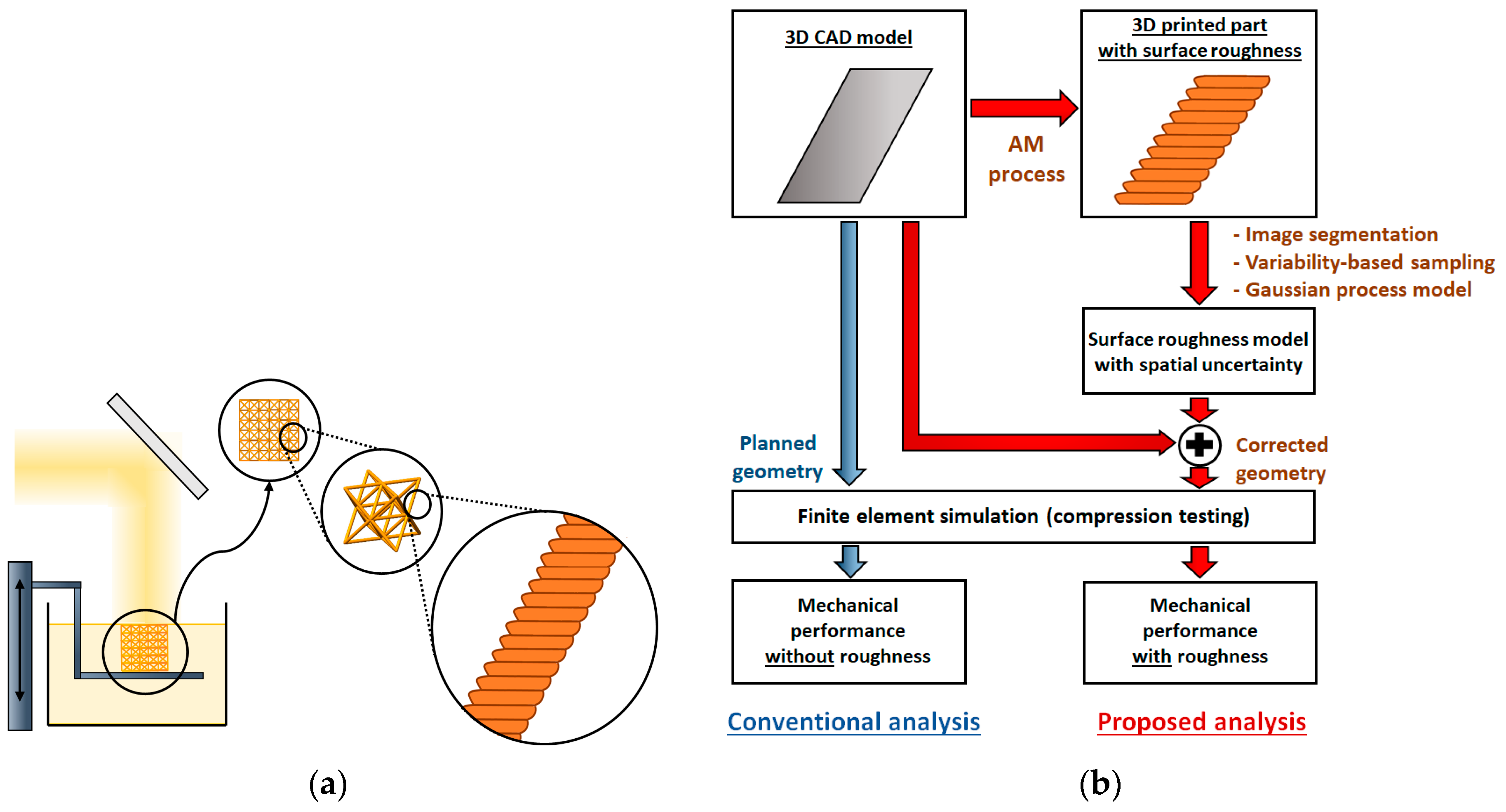
Figure 1a shows a schematic illustration of additive manufacturing process of a 3D microlattice using a mask projection stereolithography technique. The manufactured microlattice has a hierarchical structure of repeating unit cells which consist of thin struts arranged in multiple directions. In the study, we present a probabilistic modeling framework that can predict the spatial variations of printed geometry via digital images of AM parts. We limit our interest to the spatial variations of a single strut given that it is a unit building block of various types of 3D microlattices and that the load-bearing characteristics of a single strut determine the mechanical behavior of the overall lattice structure. Figure 1b shows the schematic of the proposed framework to quantify the spatial uncertainty in AM parts and incorporate spatial uncertainty in a computer simulation model to better predict the mechanical performance of the AM parts. A strut is initially additively manufactured using a mask projection stereolithography technique [15]. The sidewall profile caused by the layer-by-layer manufacturing process is extracted from a microscope image, based on which a probabilistic surface model is generated. The details of the three steps involved in generating the probabilistic model are given in the following sections.
2. Materials and Methods
2.1. Sample Fabrication
All materials including the liquid polymer, photo initiator (PI), and photo absorber (PA) are purchased from Sigma-Aldrich (St. Louis, MO, USA) and used in the as-received condition. Poly (ethylene glycol) diacrylate (PEGDA) (Mn 250) is used as a base polymer. Phenylbis (2,4,6-trimethylbenzoyl) phosphine oxide as PI and Sudan I as PA are added into the polymer at concentrations of 2 wt.% and 0.02 wt.%, respectively.
To examine the sidewall profile of AM part, CAD models of struts with angles of 60°, 75°, and 90° with respect to a horizontal plane were designed in SolidWorks. All struts are 6 mm in height and exhibit a diameter of 800 μm. Each 3D model is digitally sliced into a series of two-dimensional (2D) bitmap images with a layer thickness of 100 μm.
We used a custom-built mask projection stereolithography AM system in the study [15,16]. An ultraviolet (UV) digital projector (CEL5500, Digital Light innovations) generates spatially patterned light for each cross-sectional image, and this is projected through a 2× microscope objective lens and focused on the top surface of the liquid polymer mixture. When a layer is photopolymerized with an exposure time of 20 s, the sample holder on which the object rests is lowered by a linear stage (MTS50-Z8, Thorlabs) by a layer thickness of 100 μm. The subsequent cross-sectional image is projected to photopolymerize the next layer on top of the preceding layer. The process is repeated until all layers are completed. Each sample is individually fabricated at the center of the build area for consistency. Process parameters of the AM process, including light intensity, layer thickness, and curing time, are listed in Table 1.
Fabricated samples are rinsed in ethanol to remove the uncured polymer from the object. The prepared samples were optically inspected via a microscope. Images of the side profile of the samples were captured using a digital camera attached to the microscope.
2.2. Image Segmentation by Using a Level Set Method
The accuracy of data-driven stochastic model for spatial uncertainties depends on the experimental characterization data. Although profilometry is a fast and simple method to measure the spatial profiles, the usage of profilometry is strictly limited by its dimensional accessibility [17]. Therefore, we employ an image-based technique to extract the spatial variation of AM products. The method involves collecting sidewall profile data of additively manufactured struts from multiple sample images and extracting the data set that can be used to quantify the spatial variations by using image segmentation. The image-based technique can be applied to any spatially varying field obtained from any imaging technique.
Image segmentation is a partitioning process that groups clusters of pixels of a digital image based on parameters including their colors, intensities, and textures to extract useful information from the image [18]. Various techniques are proposed for segmenting images [18,19,20]. Among these, thresholding is one of the simplest and most widely used techniques for image segmentation. Thresholding separates pixels in which the grayscale level exceeds a critical value from the background, and the critical value is defined by the image gray-level histogram. However, a few disadvantages of thresholding are also reported, including susceptibility to pixel noise and the possibility that the extract profile is potentially not a closed contour due to lack of consideration of spatial characteristics [21]. In this study, we use the level set method to extract the profiles of objects in the image [22]. In the level set method, a higher dimensional function termed as level set function (ϕ) is defined to describe the contour. The contour evolves toward the object’s boundaries in the image based on the predefined constraints such as difference or gradient of pixel intensities. With respect to the evolving level set function, the contours are given by the zero-level set, , which evolves toward the object’s boundaries.
We assume that is the domain inside an image, and denotes the intensity of pixel at the pixel’s location . The general energy function in the level set method is shown as follows [23]:
where and denote the pixel intensity averages inside the contour and in the background region, respectively, and , , and are non-negative weighting factors. A smoothing function is selected for the robustness of the algorithm. L defines the smoothing length, and ξ locates the center of the smoothing function. The Heaviside function (H) is used to differentiate the object and the background . The physical meaning of each term in Equation (1) is as follows: The first term matches the average pixel intensity inside the contour with the pixel intensity of objects by minimizing its mean-squared error. Similarly, the second term matches the pixel intensity of background in the image. The third term regulates the smoothness of the contour, and thus a higher weight of the term implies the smoothing of the contour. The initial condition of the level set function is given by the threshold pixel intensities. With the fixed level set function, and are obtained as follows:
Given and , the energy function E is minimized by a standard gradient descent algorithm [23]. This two-step energy minimization is repeated until the converged level set function is obtained. As a result, the zero level set of the converged level set function is matched with the object’s boundaries in the image. Further details regarding the level set method is described in [23].
2.3. Variability-Based Sampling and Bisection Method
The extracted boundaries from image segmentation correspond to a uniformly distributed data set that shows the edge profile. The data can be used for the Gaussian process model. However, the number of data points in the set is proportional to the number of hyperparameters to be fitted, and thus an efficient sampling of the data set is required to reduce the computational cost and improve the convergence rate. To determine the sampling locations along the profile , the local variability, , is defined to calculate the probability of sampling at each location, , as follows [24,25]:
in which denotes a location within the region around x, denotes the local mean of the profile values in the region , and denotes the number of measurement locations in the region. The numerator, , measures the geometrical distance between x and x′ and the denominator, , makes x′ near the x more influential to the variability. averages the calculated variability. The intent behind the variability-based sampling is that the regions in which the profile varies more frequently should include more sampling locations, and thus the details within the region can be captured properly. The probability distribution for sampling as defined in Equation (4) is used, and there is a higher probability of selecting the sampling locations with higher local variability as the initial measurements.
In addition to the variability-based sampling, we also employ an iterative bisection algorithm as follows: if a certain region between two selected measurement locations exhibits a high deviation between the estimated mean and the mean from realizations, then we add an additional measurement point in the middle of the region to improve the match. The process is repeated until the deviations in the entire region are lower than the threshold value. The bisection method ensures that every detail that might be missed in the variability-based sampling is included in the sampling domain.
2.4. Gaussian Process Modeling
In the study, we employ mask projection stereolithography technique as a model AM process [15,16]. The layer-by-layer nature of the process inevitably yields a staircase sidewall profile of the part, leading to geometric difference between the manufactured part and the planned geometry (or the 3D computer model). Furthermore, when high-aspect-ratio structures, such as thin struts or beams, are manufactured, the geometric difference can also be affected by the angle between the substrate and the strut [26]. This problem is universal and found in most AM processes. In order to quantify the deviation, we consider the sidewall profiles of the AM part captured using a digital camera attached to a microscope. We assume that the extracted edge roughness profiles of AM parts result from the following two parts: (1) staircase profile: consistent curing behavior from the printing apparatus (consistent deviation between the planned geometry and actual printed geometry) and (2) spatial uncertainty (small variations): stochastic roughness variations from the AM process arising from inherent uncertainties, such as light scattering, mask projection not perfectly focused on the curing plane, perturbation on the liquid resin surface, and uncontrolled external environmental factors including fluctuations of temperature or oxygen level. After separating the effects from both the aforementioned factors, we focus on the second part, namely the spatially varying stochastic roughness uncertainty that is not a function of the printed angle.
Spatial uncertainty is often represented by a random process that is defined as a collection of random variables in space or time. In the study, we assume that the random process behind the spatial roughness uncertainty is represented by a Gaussian process [27]. The advantage of using a Gaussian process is that the random process is fully described by the mean and covariance functions, and thus it is possible to obtain the full probabilistic prediction as well as the estimation of uncertainty in the prediction.
We define the spatial uncertainty in the sidewall profile as the roughness d and assume that this uncertainty is the realization of a Gaussian process (f). The Gaussian process is a statistical model that produces a set of random variables; and the finite selection of the random values within the set follows a multivariate Gaussian distribution [27]. The Gaussian process is fully described in terms of its mean M and covariance C, and its realization is also fully specified by and in which X denotes the domain of the realization [28]. The stationary Gaussian process model for roughness spatial uncertainty is defined as follows:
where GP and N stand for the Gaussian process and normal distribution, respectively. denotes the B-spline basis function of order k, denotes the corresponding weight factor at ith location, and denotes the knot vector for the mean function [29]. The B-spline representation is used as the mean function to model the local variability in roughness. This is especially useful when the shape of the mean function is not known a priori. The Matérn covariance is used because it represents a diverse class of covariance functions that belong to the exponential family, which is commonly used to model physical stochastic processes [27]. The Matérn covariance includes three hyperparameters, namely and that control its differentiability, correlation length, and amplitude, respectively.
In order to determine the stationary Gaussian process properly, we applied the Bayesian inference approach to estimate the probability density functions (PDFs) of unknown parameters. It follows the Bayes’ theorem as follows [30]:
where Φ = is a set of unknown parameters in the Gaussian process and Pr(Φ) and Pr(Φ|d) are the prior and posterior distributions of Φ, respectively. If prior information about the distribution of the unknown parameters exists, it can be incorporated into the prior probability density functions (PDFs) of the corresponding unknown parameters [31]. Conversely, if prior information on the parameters is absent, the uniform PDFs in the certain range can be included. If each parameter is statistically independent to the others, Pr(Φ) can be expressed as a multiplication of prior distributions of each parameter. The Pr(Φ|d) is the inferred distribution of unknown parameters as a result of having the observed data. Pr(d|Φ) is the probability density of the observed data given a model parameterized with parameters Φ. This is called likelihood. Pr(d) is a normalizing term and it is often ignored because it does not affect the posterior PDFs and the computational cost for calculating this term is quite demanding. In practice, the posterior PDFs of unknown parameters are proportional to the multiplication of the prior PDFs and the likelihood. In this work, we used the multivariate normal distribution as the likelihood and the uniform distribution for prior PDFs of unknown parameters. The sampled data from the variability-based sampling and bisection algorithm is used as the observed data, d.
Since it is not always possible to estimate the closed form for the posterior PDFs of unknown parameters and calculation of the posterior PDFs involves high dimensional integration. Therefore, the sampling-based approach, called the Markov Chain Monte Carlo (MCMC) algorithm, is used to estimate the posterior PDFs of unknown parameters in this study [30,32]. The convergence of posterior PDFs of unknown parameters is determined by inspecting the trace of each estimating parameter from the sampling. A high value is chosen as the number of iteration of MCMC sampling, so that it ensures the trace of each estimating parameter shows an asymptotic behavior. The asymptotic behavior stands for the state that the mean and the variance of sample stay unchanged. The open-source Bayesian analysis package PyMC [32] is used to perform Monte Carlo sampling to estimate the posterior PDFs of unknown parameters.
3. Results
3.1. Gaussian Process Modeling and Sampling Algorithm Verification
We present a test problem to illustrate and verify our Gaussian process modeling with the variability-based sampling and bisection algorithm. Equation (7) is the mathematical form of the given mean function q and is expressed as follows:
The linear slope between the starting and ending points of the function is removed since locally varying spatial variation is the main focus. We decide to use Equation (7) that has a higher spatial variation frequency in the region when compared to that in region to test whether our algorithm captures the correct behavior of spatial roughness variation when its characteristics are not uniform over the entire domain. A Matérn covariance function with the parameters: ν = 2, ϕ = 2, θ = 0.4 is used to generate the spatial variation. We generate realizations of the random process and sample these realizations at a total of 61 measurement locations. The sampled data is used as the input for estimation, wherein we try to reconstruct the parameters of the actual stochastic process from which the data originated. We assign the following prior PDFs for the unknown parameters:
The prior PDFs can be specifically selected to incorporate any knowledge regarding the values of the unknown parameters. Otherwise, they can be set as uniform distribution in the absence of the aforementioned information. We use 500 realizations of the given random process that are sampled at the given locations to generate the joint posterior distribution of the parameters and select 1000 samples from it using the Markov chain Monte Carlo method with a burn-in of 30,000 and a thinning factor of 10 [17].
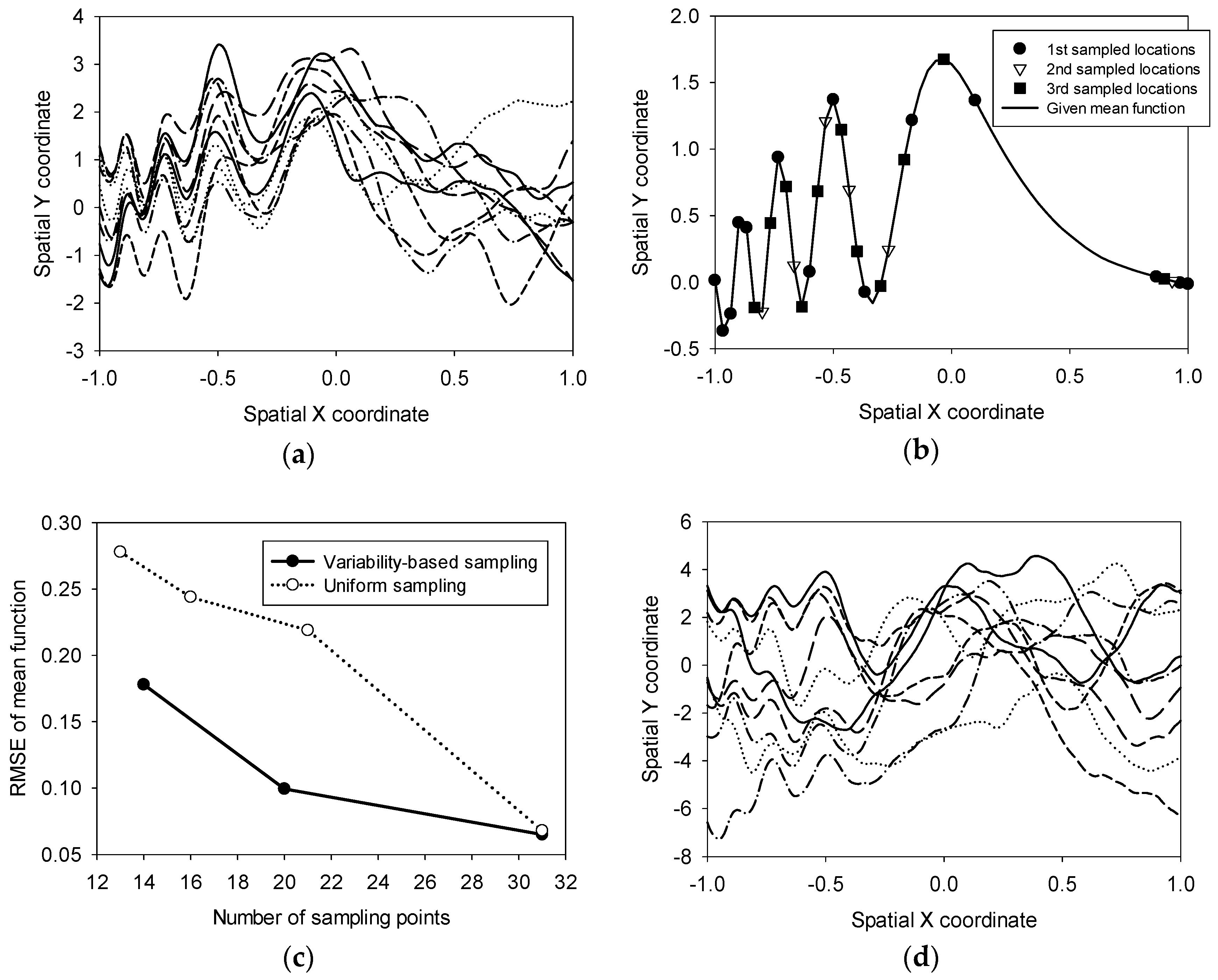
Figure 2a shows 10 realizations from the given stochastic process. The sampled points in the 1st (circles), 2nd (triangles), and 3rd (rectangles) runs of non-uniform sampling are also shown in Figure 2b. Fourteen points from the 1st sampling based on the local variability effectively capture the high frequency spatial variation near the left sidewall. However, they miss a few details near the left sidewall as well as near the right sidewall. The lack of sampling points is compensated in the 2nd and 3rd bisection steps by placing additional sampling points and reducing the deviation between the mean function calculated from all realizations and the estimated mean function. Total sampled points in the 2nd and 3rd sampling from the bisection method are 20 and 31, respectively.
To visualize the effectiveness of variability-based sampling and the bisection algorithm, the root-mean-square error (RMSE) between the estimated mean and the mean from realizations is calculated and compared in two different sampling cases: proposed variability-based sampling and uniform sampling. The result is shown in Figure 2c. The x-axis denotes the number of sampling points and the y-axis denotes the RMSE value. Given the efficient placement of measurement locations, the RMSE in non-uniform sampling is considerably lower than that in the uniform sampling result with an equal number of sampling points. Additionally, while the RMSE is reduced with increases in the sampling locations, the RMSE decreases significantly faster in the variability-based method. The RMSEs in both methods are identical when the sampling locations correspond to almost half of the total measurement locations. Therefore, we conclude that variability-based sampling and the bisection algorithm is a more attractive option for the effective allocation of computing power and resources. Figure 2d shows 10 sampled realizations from the estimated Gaussian process model.
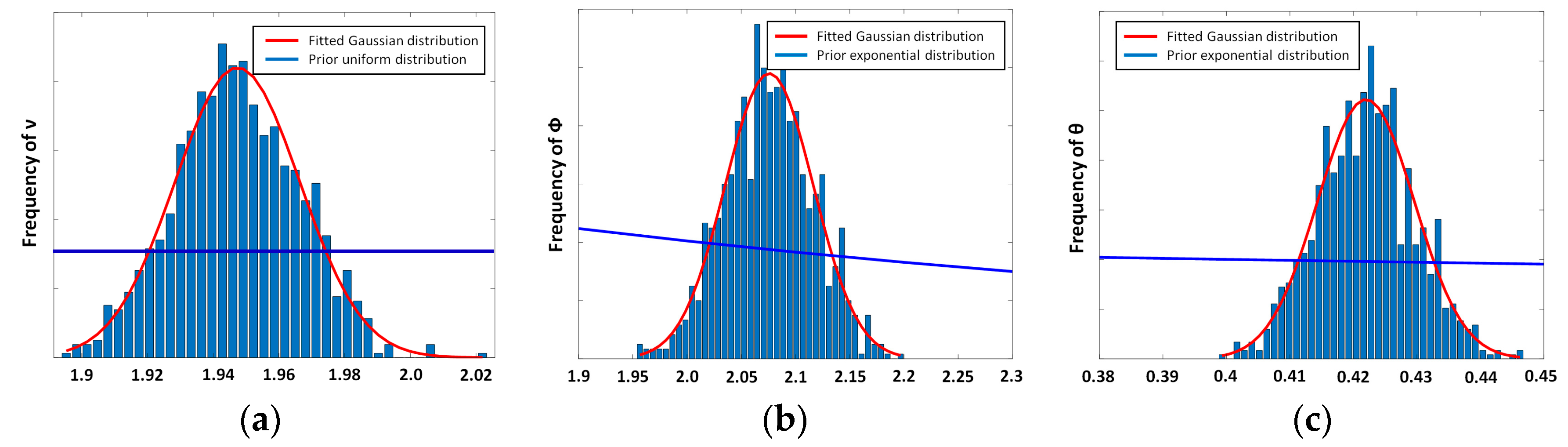
In addition to the comparison of the mean function, the estimated parameters in the Matérn covariance function with respect to the number of sampling points are shown in Table 2. There are three parameters in the Matérn covariance function, and the given values are denoted in the parentheses. In contrast to the deviations in the mean function, the estimated parameters do not significantly depend (within a 5% error) on the number of sampling points. It can be speculated that the sampled points from the variability-based sampling gives enough information to accurately estimate the hyperparameters in the covariance function even though it missed a few local variabilities in the mean function. Figure 3 shows the prior and the posterior PDFs of three unknown parameters in the Matérn covariance function. The prior PDF from Equation (8) is displayed with a blue line at the displayed region and the blue histogram is from the posterior PDF obtained by histogram of the trace values from MCMC sampling. The red line is a fitted normal distribution to the histogram. Figure 3 clearly visualizes the updating process of Bayesian inference by incorporating the observed data. It is important to emphasize that since the estimated parameters are obtained as PDFs instead of single values, the Gaussian process described by the estimated parameters is a set of multiple Gaussian processes defined by hyperparameters realized from the posterior PDFs. This helps us to model a wide range of uncertainties in the observed data while keeping the practical advantages of Gaussian process.
3.2. Extracting Profiles from the Images of Additively Manufactured Struts.
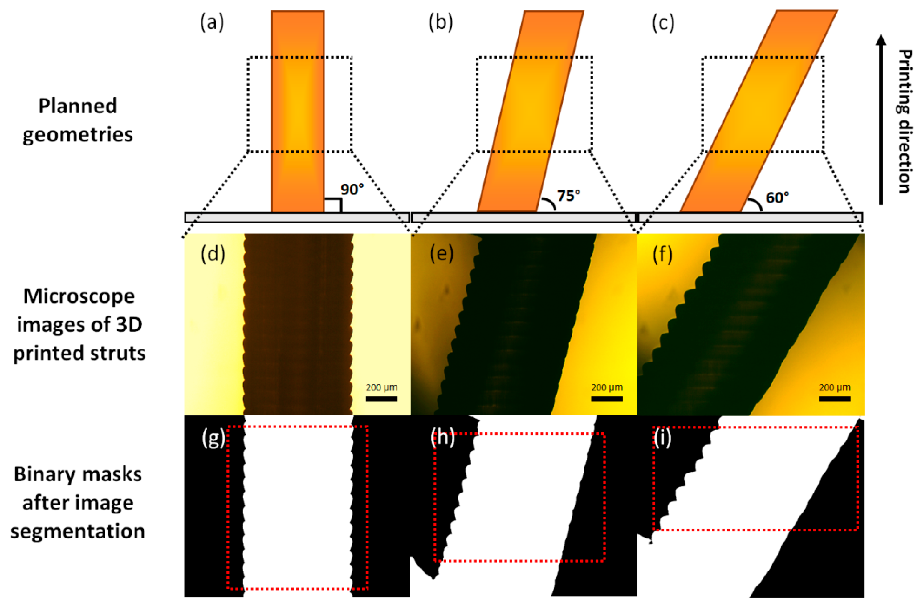
Gaussian process modeling with the non-uniform sampling algorithm is applied to the sidewall profiles of AM fabricated struts. Figure 4a–c shows the CAD geometries of struts in 3 different printing angles (90°, 75°, and 60°) and printing directions. The layer thickness corresponds to 80 pixel units. The sidewall profiles of multiple AM fabricated struts with different angles (90°, 75°, and 60°) are shown in Figure 4d–f. The sidewall profile consists of multiple layers printed repeatedly layer-by-layer, and we assume that the spatial uncertainty in each printed layer is generated from an independent event, so that is not related to the neighboring layers. There are three parameters in Equation (1) that are reduced by considering the two ratios, and . We manually segmented one printed layer in the image and varied the two ratios to determine the optimized parameter values to obtain the optimal match with respect to the manually segmented edge. After calibrating two ratios in the level set method, the same algorithm is applied to the remaining layers to extract the edge information from the image.
Figure 4g–i shows the binary masks of the images after segmentation in which the white pixels represent the segmented region of the strut and the black pixels denote the background region. Given the smooth intensity gradient from the center to the edge of the image, the segmentation at the edges of the images is inaccurate in the 75° and 60° cases in Figure 4h,i. The artifact from the background inhomogeneity can be easily removed by measuring and compensating the intensity gradient in the background. The compensation is not applied in the study to minimize the manual intervention. A more systematic approach to reduce the effect from the local inhomogeneity is given in [33].
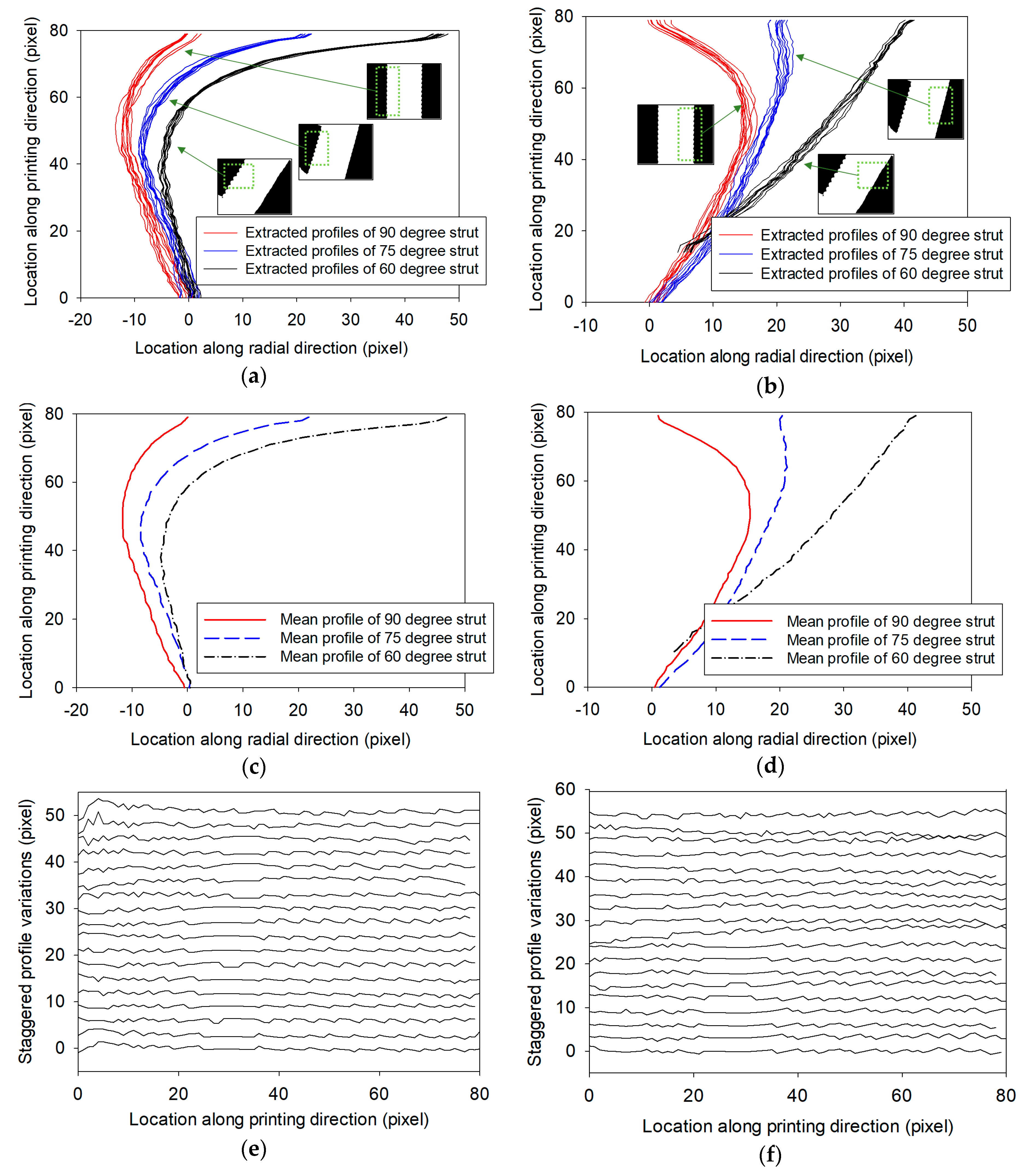
The edge profile is extracted by collecting the outermost pixels in the left and right sidewalls of binary masks. Figure 5a,b shows the extracted edge profiles in the left and right sidewalls of each printed layer, respectively. It is clear that the side profile of all layers show consistent trend depending on the printing angle. This characteristic staircase profile is caused by the light absorption and scattering in the resin vat and light penetration during the curing of upper layer. In a manner similar to the test case, the mean of all observations, which represents the staircase profile, is subtracted from the sidewall profile; thus, the roughness spatial uncertainty is independent of the printed angle. The mean profile is obtained by simple summation of all side profiles in each printing angles. The summation averages out the local roughness from the mean profile. The mean trends extracted from all observations and the roughness extracted spatial uncertainties are shown in Figure 5c–f, respectively. In total, 37 roughness profiles are collected and the roughness is independent of printing angle as well as direction of side profile as shown in the Figure. This will be used for estimating hyperparameters in the Gaussian process model.
In contrast to the test case, we possess prior information on the distribution of the amplitude and scaling parameters of covariance function from the geometrical constraints of the printed struts. Based on the roughness spatial variation amplitude from observations, the upper limit on the prior distribution of the amplitude parameter in the covariance function is 5. Additionally, the maximum correlation length is limited up to the height of a printed layer. Equation (9) describes the prior information of the hyperparameters.
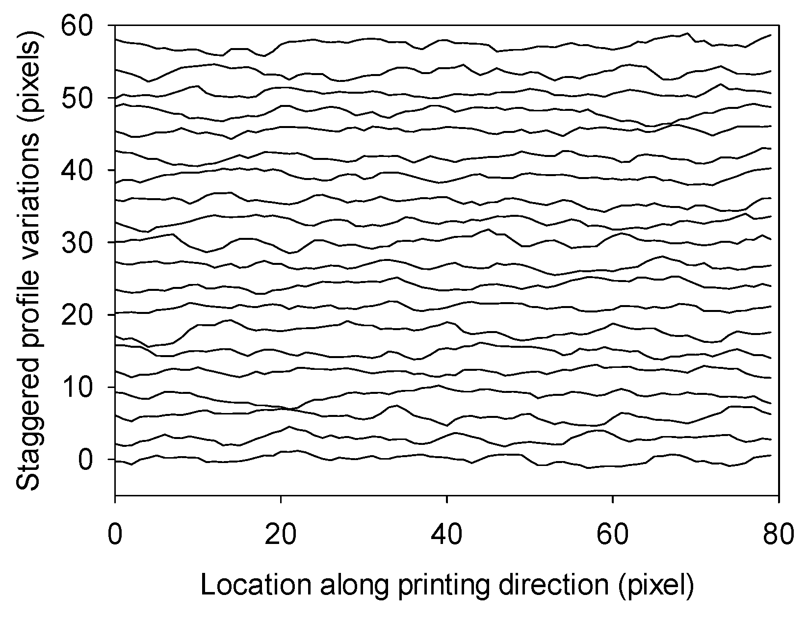
Twenty realizations from the estimated stochastic model are shown in Figure 6. In a manner similar to the observations from the extracted profiles of actual struts, the fluctuations are distributed uniformly over the domain, and this indicates the characteristics of the stationary Gaussian process. This reproduced roughness will be superimposed in the CAD geometry with the mean profile to quantify the effect of side profile on the mechanical behavior of AM parts.
3.3. Effect of Spatial Uncertainty on the Mechanical Behavior of Additively Manufactured Struts
In the study, we consider simple struts with three different printing angles (90°, 75°, and 60°). In order to clearly visualize the effect from the spatial uncertainty, the struts in FE analysis are simplified as 2D struts. To investigate the effect of spatial uncertainty on the mechanical properties of additively manufactured struts, three computational models with different strut geometries are first prepared as follows: (1) nominal strut: desired CAD geometry with a smooth side surface (planned geometry without any staircase profile as well as spatial uncertainty), (2) predicted AM strut: geometry with predicted roughness in which the staircase profile and the spatial uncertainty are reproduced from our estimated Gaussian process model, and (3) volume-matched strut: strut also with a smooth side surface, having a thickness adjusted by smoothing the ridges and valleys of the rough side profile such that the volume is matched with the predicted AM strut. The analysis of (3) is necessary for fair comparison because the thickness of the manufactured struts is slightly lower than that of the planned geometry. By including (3), the difference in the mechanical properties that are caused by the volume change can be investigated. The thickness of the strut in the CAD model is 800 μm, and the thicknesses of struts in the volume-matched geometries extracted from the sample images are approximately 754 μm, 754 μm, and 760 μm for 90°, 75°, and 60°, respectively. For the computational efficiency, one third of the height of printed strut (2000 μm) is modeled in the simulation. The three different aforementioned geometries are created for each printing angle, namely 90°, 75°, and 60°.
A linear static structural analysis was performed to calculate the mechanical property of struts in three different printing angles (90°, 75°, and 60°) under compressional loading conditions. A commercial FE software package, COMSOL MultiphysicsTM, running on the personal computer (Windows 10 64 bit, Intel i7-4790 CPU, 16 GB RAM), was used for all numerical simulations. The governing equation for the struts is as follows [34]:
where F is the deformation gradient, S is the second Piola–Kirchhoff stress, v is the left stretch tensor. The Cauchy stress tensor, , is the multiplication of F, S, the transpose of F, and the volume ratio, J, which is the determinant of F. The Lagragian–Green strain, , is a function of F and the identity tensor, I. The second Piola–Kirchhoff stress, S, is the gradient of the strain energy-density function, Ws with respect to . is the scalar invariant of the left Cauchy–Green deformation tensor. The struts are made of a photo-polymerizable poly(ethylene glycol) diacrylate (PEGDA) (molecular weight 250). PEGDA is assumed to be a hyperelastic, incompressible, and isotropic material and modeled by using neo-Hookean model [34]. The uniaxial compression test is performed to obtain the material property of PEGDA. The stress–strain curve obtained from the experiment is fitted to the neo-Hookean model to determine the shear modulus, µ. The fitted value of µ is approximately 36.1 MPa for the PEGDA.
The interfacial boundaries of each layer were merged together with its neighboring layers using “union assembly” feature in COMSOL software, assuming the perfect binding condition between layers. Zero-displacement was imposed on the bottom of the strut, and the controlled displacement was applied on the top surface of the strut in the vertical direction as described in Equation (11).
where u is the displacement vector in the computational domain and is the displacement vector of elements at the bottom of strut. is the vertical displacement of elements at the top of the strut and is the controlled displacement that was applied as a boundary condition.
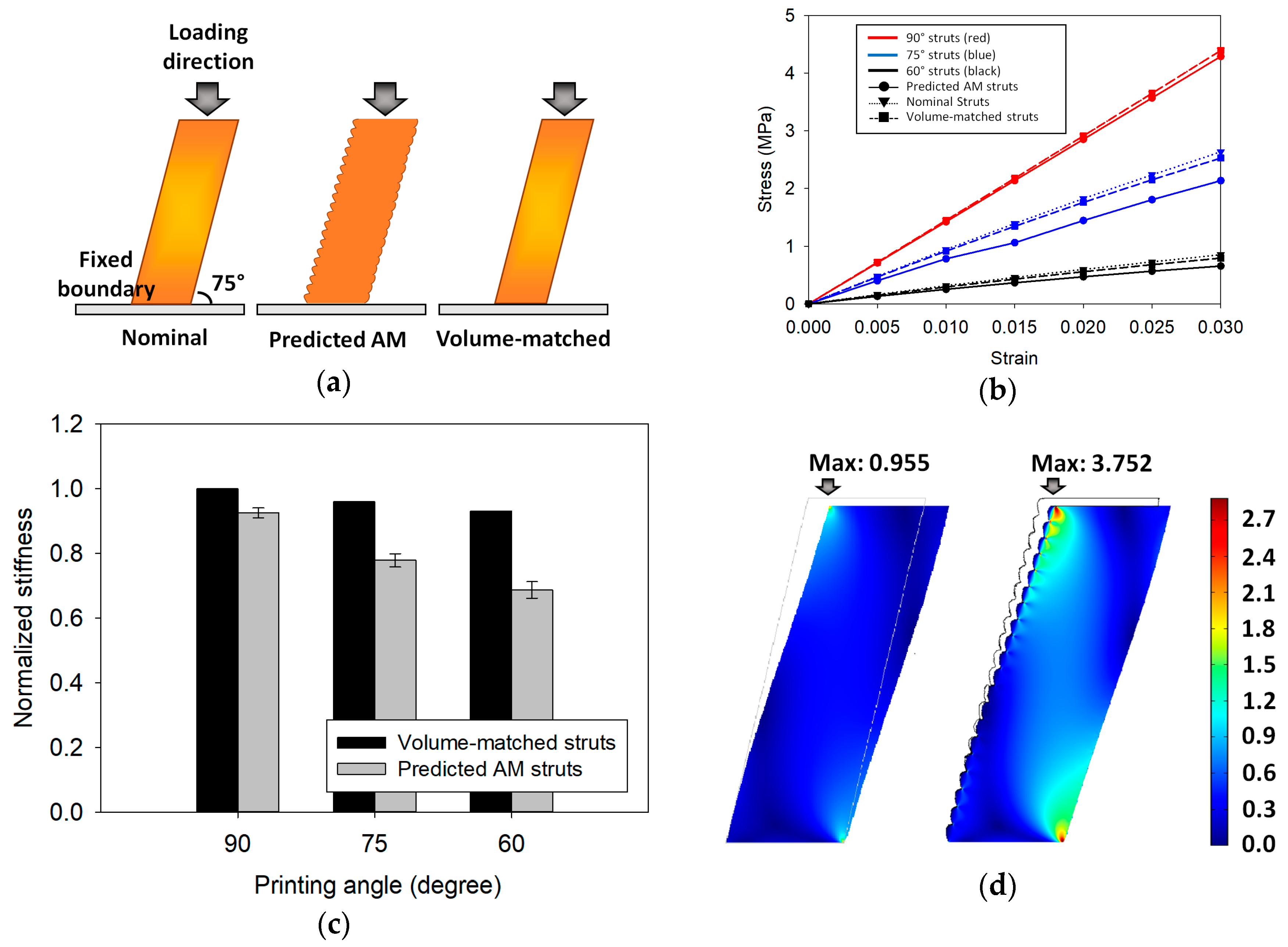
Figure 7a shows the loading direction and the boundary condition in the three struts: nominal, predicted AM, and volume matched struts. The applied strain was limited up to 0.03 to avoid the nonlinear deformation of the strut. Since the strut is considered as the building block of unit cell structure, the strain is defined as the actual deformation of the strut divided by the height of the strut. With respect to the deformation of the strut, the resulting stress was calculated as the average of total pressure over the bottom surface of the strut. Triangular elements as well as the adaptive mesh size control were adopted to make sure that it captures all details of spatial uncertainties at the edge of struts. The mesh size convergence test was performed to ensure that the simulation result is not sensible to the mesh size. The number of elements in three different geometries, giving the consistent simulation results, are 10,040, 831,944, and 9474 for the nominal strut, predicted AM strut, and volume-matched strut, respectively. The number of elements for predicted AM strut is significantly higher than the others because of the geometrical details of spatial uncertainty at the edge of strut.
Figure 7b shows the stress–strain curves of 9 different examples obtained from the FE simulation. The slope of the stress–strain curve denotes the stiffness of the strut. The slopes of all stress–strain curves are grouped into three categories based on its printing angle, and a slope deviation exists given the existence of the spatial deviation. The decrease in slope is qualitatively observed in the predicted AM strut and volume-matched strut. To quantitatively understand the effect of spatial deviation on the stiffness of the struts, the stiffness of the volume-matched and predicted AM struts are normalized with the stiffness of the nominal struts as shown in Figure 7c. The change in the effective stiffness of the volume-matched geometry is not significant (less than 7% of the stiffness of the nominal) when the printing angle changes from 90° to 60°. However, when the geometry exhibits roughness including the staircase profile as well as the spatial uncertainty, the stiffness is reduced to 70% of the nominal geometry when the printing angle is 60°. The reduction in stiffness is expected since the roughness decreases the cross-sectional area of each strut and decreases the stiffness of the strut. However, it is observed that the roughness effect is more pronounced when compared the reduction in volume-matched case to the predicted AM case. This result indicates that the necessity of details of surface roughness becomes more important as the printing angle reduces. Specifically, the angled strut is frequently used in the lattice structures, which is the assembly of multiple unit cells, consisting of angled struts. Therefore, modeling the surface roughness including spatial uncertainty is important for the accurate estimation of mechanical properties of the lattice structure.
Additionally, we compare the maximum value of von Mises stress in the three cases. Table 3 shows the maximum von Mises stresses of the volume-matched geometry strut and the predicted AM strut normalized with respect to the maximum von Mises stress of the nominal strut. The von Mises stress distribution and the location of the maximum value is displayed in Figure 7d. The stress distribution in Figure 7d shows distinctive difference from the stress distribution in the vertical strut because of two major factors: (1) bending and shear stresses and (2) surface roughness. When a strut is loaded axially, it only develops compressive normal stress. When a strut is loaded with an angle, bending and shear stresses begin to arise, and it becomes more likely that the strut undergoes a large deformation and becomes more susceptible to developing a large stress as shown in Figure 7d. In addition to the effect from bending and shear stresses, local stress concentrations are observed near the side profiles in the predicted AM, which is not observed in the volume-matched strut or the nominal strut in which the sidewall profiles are smooth. The geometric discontinuities caused by the spatial uncertainties change the stress distribution in the strut, and the amount of stress concentration is thrice that in the smooth cases. Thus, it is anticipated that the total stiffness of the additively manufactured strut is affected by the change in stress distribution. Therefore, considering spatial uncertainties in the geometry to accurately predict the mechanical behavior of struts using FE analysis is essential.
The proposed modeling framework is also applicable to complex AM parts with inner structures. The spatial uncertainties can be estimated by the proposed modeling framework if the inner structure of the complex AM parts is expected to exhibit spatial uncertainties that are statistically similar to the outer structure. Even if the inner structures of the complex AM parts are expected to exhibit statistically different spatial uncertainties, the proposed modeling framework can be still applied to the complex AM parts with the exception of the image segmentation sub-step. As opposed to the use of optical images, there are multiple techniques to measure the inner structure profile of the complex parts, such as X-ray computed tomography and profilometry. Following the extraction of the inner structure profile, it is possible to apply the remaining sub-steps of the proposed modeling framework, namely variability-based sampling and Gaussian process modeling, to the problem.
4. Conclusions
The study presents a general method to model spatial variations of additively manufactured products from their sidewall profile images. Specifically, this can be achieved using three approaches: (1) Gaussian process modeling using Bayesian framework, (2) level set method for image segmentation, and (3) variability-based sampling algorithm. The method is verified via a test problem and applied to the real AM products fabricated by mask projection stereolithography. In order to verify the necessity of the proposed framework, the mechanical properties of printed high-aspect-ratio struts with and without roughness is simulated under compression loading via FE simulation. The FE simulation results show that the staircase profile with the spatial uncertainty reduces the stiffness of printed strut to 70% when the printing angle is 60°. It is also shown that the effect from the spatial roughness increases as the printing angle decreases. This indicates that the accurate estimation of mechanical behavior of AM products as well as lattice structures consisting of multiple angled struts requires to consider the spatial roughness. In addition, the influence from the spatial roughness significantly affects the stress distribution under compressive loading conditions that could result in the location of failure in the structure. It is also expected that the effect from roughness is more significant when the dimension of AM structures approaches the magnitude of roughness. The proposed modeling framework can be applied to complex AM parts which have spatial roughness that can be measured through optical images. The proposed method is not limited to AM products, and it can be applied to other problems in which spatial variations exist and its mechanical behavior is expected to be affected by its spatial roughness.
Author Contributions
Conceptualization, N.K., H.L. and N.A.; Data curation, N.K. and C.Y.; Formal analysis, N.K.; Funding acquisition, H.L. and N.A.; Investigation, N.K.; Methodology, N.K. and C.Y.; Supervision, H.L. and N.A.; Visualization, C.Y.; Writing–original draft, N.K.; Writing–review & editing, C.Y., H.L. and N.A.
Funding
This research was funded by the National Science Foundation under grant number 1420882. We also acknowledge the support of DMDII. Additionally, we acknowledge support from the Agency for Defense Development under contract number UD150032GD.
Conflicts of Interest
The authors declare no conflict of interest.
References
- Melchels, F.P.W.; Feijen, J.; Grijpma, D.W. A review on stereolithography and its applications in biomedical engineering. Biomaterials 2010, 31, 6121–6130. [Google Scholar] [CrossRef] [PubMed] [Green Version]
- Alapan, Y.; Hasan, M.N.; Shen, R.; Gurkan, U.A. Three-dimensional printing based hybrid manufacturing of microfluidic devices. J. Nanotechnol. Eng. Med. 2015, 6, 021007. [Google Scholar] [CrossRef] [PubMed]
- Zheng, X.; Lee, H.; Weisgraber, T.H.; Shusteff, M.; DeOtte, J.; Douss, E.B.; Kuntz, J.D.; Biener, M.M.; Ge, Q.; Jackson, J.A. Ultralight, ultrastiff mechanical metamaterials. Science 2014, 344, 1373–1377. [Google Scholar] [CrossRef] [PubMed] [Green Version]
- Bauer, J.; Meza, L.R.; Schaedler, T.A.; Schwaiger, R.; Zheng, X.; Valdevit, L. Nanolattices: An emerging class of mechanical metamaterials. Adv. Mater. 2017, 29, 1701850. [Google Scholar] [CrossRef] [PubMed]
- Schaedler, T.A.; Ro, C.J.; Sorensen, A.E.; Eckel, Z.; Yang, S.S.; Carter, W.B.; Jacobsen, A.J. Designing metallic microlattices for energy absorber applications. Adv. Eng. Mater. 2014, 16, 276–283. [Google Scholar] [CrossRef]
- Frenzl, T.; Findeisen, C.; Kadic, M.; Gumbsch, P.; Wegener, M. Tailored buckling microlattices as reusable light-weight shock absorbers. Adv. Mater. 2016, 28, 5865–5870. [Google Scholar] [CrossRef] [PubMed]
- Dejean, T.T.; Spierings, A.B.; Mohr, D. Additively-manufactured metallic micro-lattice Materials for high specific energy absorption under static and dynamic loading. Acta Materialia 2016, 116, 14–28. [Google Scholar] [CrossRef]
- Roper, C.S.; Fink, K.D.; Lee, S.T.; Kolodzijeska, J.A.; Jacobsen, A.J. Anisotropic convective heat transfer in microlattice materials. AIChE J. 2013, 59, 622–629. [Google Scholar] [CrossRef]
- Maloney, K.J.; Fink, K.D.; Schaedler, T.A.; Kolodzijeska, J.A.; Jacobsen, A.J.; Roper, C.S. Multifunctional heat exchangers derived from three-dimensional micro-lattice structures. Int. J. Heat Mass Tranf. 2012, 55, 2486–2493. [Google Scholar] [CrossRef]
- Warnke, P.H.; Doyglas, T.; Wolny, P.; Sherry, E.; Steiner, M.; Galonska, S.; Becker, S.T.; Springer, I.N.; Wiltfang, J.; Sivananthan, S. Rapid prototyping: Porous titanium alloy scaffolds produced by selective laser melting for bone tissue engineering. Tissue Eng. Part C Methods 2008, 15, 115–124. [Google Scholar] [CrossRef]
- Ahn, D.; Kim, H.; Lee, S. Surface roughness prediction using measured data and interpolation in layered manufacturing. J. Mater. Process. Technol. 2009, 209, 664–671. [Google Scholar] [CrossRef]
- Ancau, M.; Caizar, C. The optimization of surface quality in rapid prototyping. In Proceedings of the WSEAS International Conference on Engineering Mechanics, Structures, Engineering Geology, Heraklion, Crete Island, Greece, 22–24 July 2008. [Google Scholar]
- Hasan, R. Progressive Collapse of Titanium Alloy Micro-Lattice Structures Manufactured Using Selective Laser Melting. Ph.D. Thesis, University of Liverpool, Liverpool, UK, 2013. [Google Scholar]
- Meza, L.R.; Greer, J.R. Mechanical characterization of hollow ceramic nanolattices. J. Mater. Sci. 2014, 49, 2496–2508. [Google Scholar] [CrossRef]
- Zheng, X.; Deotte, J.; Alomso, M.P.; Farquar, G.R.; Weisgraber, T.H.; Gemberling, S.; Lee, H.; Fang, N.; Spadaccini, C.M. Design and optimization of a light-emitting diode projection micro-stereolithography three-dimensional manufacturing system. Rev. Sci. Inst. 2012, 83, 125001. [Google Scholar] [CrossRef]
- Sun, C.; Fang, C.; Wu, D.M.; Zhang, X. Projection micro-stereolithography using digital micro-mirror dynamic mask. Sens. Actuators A Phys. 2005, 121, 113–120. [Google Scholar] [CrossRef] [Green Version]
- Alwan, A.; Aluru, N.R. Data-driven stochastic models for spatial uncertainties in micromechanical systems. J. Micromech. Microeng. 2015, 25, 115009. [Google Scholar] [CrossRef] [Green Version]
- Pal, N.R.; Pal, S.K. A review on image segmentation techniques. Pattern Recognit. 1993, 26, 1277–1294. [Google Scholar] [CrossRef]
- Shapiro, L.; Stockman, G.C. Computer Vision; Prentice Hall: New Jersey, NJ, USA, 2001. [Google Scholar]
- Cremers, D.; Rousson, M.; Deriche, R. A review of statistical approaches to level set segmentation: Integrating color, texture, motion and shape. Int. J. Comput. Vis. 2007, 72, 195–215. [Google Scholar] [CrossRef]
- Sahoo, P.K.; Soltani, S.; Wong, A.K.C. A survey of thresholding techniques. Comp. Vis. Graph. Image Process. 1988, 41, 233–260. [Google Scholar] [CrossRef]
- Osher, S.; Sethian, J.A. Fronts propagating with curvature-dependent speed: Algorithms based on hamilton-jacobi formulations. J. Comput. Phys. 1988, 79, 12–49. [Google Scholar] [CrossRef]
- Chan, T.F.; Vese, L.A. Active contours without edges. IEEE Trans. Image Process. 2001, 10, 266–277. [Google Scholar] [CrossRef] [Green Version]
- Anderson, A.B.; Wang, G.; Gertner, G. Local variability based sampling for mapping a soil erosion cover factor by co-simulation with landsat tm images. Int. J. Remote Sens. 2006, 27, 2423–2447. [Google Scholar] [CrossRef]
- Jin, R.; Chang, C.J.; Shi, J. Sequential measurement strategy for wafer geometric profile estimation. IIE Trans. 2012, 44, 1–12. [Google Scholar] [CrossRef]
- Kim, N.; Bhalerao, I.; Han, D.; Yang, C.; Lee, H. Improving surface roughness of additively manufactured parts using a photopolymerization model and multi-objective particle swarm optimization. Appl. Sci. 2019, 9, 151. [Google Scholar] [CrossRef]
- Rasmussen, C.E. Gaussian processes for machine learning. In Lecture Notes in Computer Science; Springer: Berlin/Heidelberg, Germany, 2006; pp. 63–71. [Google Scholar]
- Cressie, N. Statistics for Spatial Data; Wiley Series in Probability and Statistics; John Wiley and Sons Ltd.: New York, NY, USA, 1993. [Google Scholar]
- De Boor, C. A Practical Guide to Splines; Springer: New York, NY, USA, 1978; Volume 27. [Google Scholar]
- Bishop, C.M. Pattern Recognition and Machine Learning; Springer: New York, NY, USA, 2006. [Google Scholar]
- Alwan, A.; Aluru, N.R. A nonstationary covariance function model for spatial uncertainties in electrostatically actuated microsystems. Int. J. Uncertain. Quantif. 2015, 5. [Google Scholar] [CrossRef]
- Patil, A.; Huard, D.; Fonnesbeck, C.J. Pymc: Bayesian stochastic modelling in python. J. Stat. Softw. 2010, 35, 1. [Google Scholar] [CrossRef]
- Wang, X.F.; Huang, D.S.; Xu, H. An efficient local chan–vese model for image segmentation. Pattern Recognit. 2010, 43, 603–618. [Google Scholar] [CrossRef]
- Asaro, R.; Lubarda, V. Mechanics of Solids and Materials; Cambridge University Press: Cambrige, UK, 2006. [Google Scholar]
Figure 1.
Schematic description of probabilistic modeling framework for an additively manufactured part: (a) Manufacturing process of a microlattice structure: a hierarchical structure of a unit cell consisting of multiple struts; (b) A probabilistic modeling framework for surface roughness estimation and mechanical behavior of an additively manufactured geometry.

Figure 2.
Given and estimated stochastic processes: (a) 10 realizations from the given model; (b) Given mean function (solid line) and sampled points in 1st (circle), 2nd (triangle), and 3rd (rectangle) runs after variability-based sampling algorithm; (c) root-mean-square error (RMSE) of the mean function from uniform and variability-based sampling algorithm; (d) 10 sampled realizations from the estimated Gaussian process model.

Figure 3.
Probability density functions (PDFs) of the estimated parameters in Matérn covariance function: (a) ν, (b) ϕ, and (c) θ. The blue line is a part of the given prior PDF at the displayed region and blue histogram is the frequency of sampled parameters from the posterior PDF. The red curve is a fitted normal distribution to the histogram. The histograms and the prior PDFs are not in the same scale.

Figure 4.
Microscope images and corresponding binary images of additively manufactured struts: (a–c) CAD geometries of struts in different printing angles (90°, 75°, and 60°); (d–f) Microscope images of additively manufactured struts (90°, 75°, and 60°); (g–i) Binary masks after image segmentation (90°, 75°, and 60°). The sidewall profiles in the red box (dotted line) are used for characterizing the spatial uncertainty.

Figure 5.
Extracted sidewall profiles of additively manufactured struts: (a) The extracted left-sidewall profiles in different angles (90°, 75°, and 60°); (b) The extracted right-sidewall profiles in different angles (90°, 75°, and 60°); (c) Extracted left-sidewall mean profiles in different angles (90°, 75°, and 60°); (d) Extracted right-sidewall mean profiles in different angles (90°, 75°, and 60°); (e) Extracted left-sidewall roughness profiles after clean-up; (f) Extracted right-sidewall roughness profiles after clean-up.

Figure 6.
Twenty sampled realizations from the estimated Gaussian process model.

Figure 7.
Compression test results of additively manufactured struts: (a) Loading and boundary conditions of three struts: nominal, predicted AM, and volume matched struts; (b) Stress–strain curve of nominal, predicted AM, and volume-matched struts in different printing angles (90°, 75°, and 60°); (c) Normalized effective stiffness of volume-matched geometry and predicted AM struts in different printing angles (90°, 75°, and 60°); (d) Normalized von Mises stress distributions in a predicted AM strut and a volume-matched strut.


Table 1.
Mask projection stereolithography process parameters.
| Total Number of Layer | 60 |
|---|---|
| Layer thickness (μm) | 100 |
| Curing time per layer (sec) | 20 |
| Light intensity (mW/cm2) | 1 |
Table 2.
Estimated hyperparameters in the covariance function for the test problem. The given values are denoted in the parentheses.
Table 2.
Estimated hyperparameters in the covariance function for the test problem. The given values are denoted in the parentheses.
| ν (2) | ϕ (2) | θ (0.4) | |
|---|---|---|---|
| 1st sampled locations (14 points) | 2.011 ± 0.027 | 2.052 ± 0.028 | 0.416 ± 0.012 |
| 2nd sampled locations (20 points) | 1.978 ± 0.025 | 2.063 ± 0.030 | 0.418 ± 0.009 |
| 3rd sampled locations (31 points) | 1.971 ± 0.016 | 2.055 ± 0.029 | 0.415 ± 0.007 |
Table 3.
Maximum von Mises stress of the volume-matched struts and the predicted AM struts normalized with respect to those of the nominal struts in different printed angles.
Table 3.
Maximum von Mises stress of the volume-matched struts and the predicted AM struts normalized with respect to those of the nominal struts in different printed angles.
| Angles | 90° | 75° | 60° | |
|---|---|---|---|---|
| Struts | ||||
| Volume-matched struts | 0.975 | 0.955 | 0.947 | |
| Predicted AM struts | 3.410 | 3.752 | 3.273 | |
© 2019 by the authors. Licensee MDPI, Basel, Switzerland. This article is an open access article distributed under the terms and conditions of the Creative Commons Attribution (CC BY) license (http://creativecommons.org/licenses/by/4.0/).
Share and Cite
MDPI and ACS Style
Kim, N.; Yang, C.; Lee, H.; Aluru, N.R. Spatial Uncertainty Modeling for Surface Roughness of Additively Manufactured Microstructures via Image Segmentation. Appl. Sci. 2019, 9, 1093. https://0-doi-org.brum.beds.ac.uk/10.3390/app9061093
AMA Style
Kim N, Yang C, Lee H, Aluru NR. Spatial Uncertainty Modeling for Surface Roughness of Additively Manufactured Microstructures via Image Segmentation. Applied Sciences. 2019; 9(6):1093. https://0-doi-org.brum.beds.ac.uk/10.3390/app9061093
Chicago/Turabian StyleKim, Namjung, Chen Yang, Howon Lee, and Narayana R. Aluru. 2019. "Spatial Uncertainty Modeling for Surface Roughness of Additively Manufactured Microstructures via Image Segmentation" Applied Sciences 9, no. 6: 1093. https://0-doi-org.brum.beds.ac.uk/10.3390/app9061093
Note that from the first issue of 2016, this journal uses article numbers instead of page numbers. See further details here.