Timbre Preferences in the Context of Mixing Music


The MARCS Institute for Brain, Behaviour and Development, Western Sydney University, Penrith, NSW 2751, Australia
*
Author to whom correspondence should be addressed.
Appl. Sci. 2019, 9(8), 1695; https://0-doi-org.brum.beds.ac.uk/10.3390/app9081695
Submission received: 21 March 2019
/
Revised: 15 April 2019
/
Accepted: 16 April 2019
/
Published: 24 April 2019
(This article belongs to the Special Issue Psychoacoustic Engineering and Applications)
Abstract
:Mixing music is a highly complex task. This is exacerbated by the fact that timbre perception is still poorly understood. As a result, few studies have been able to pinpoint listeners’ preferences in terms of timbre. In order to investigate timbre preference in a music production context, we let participants mix multiple individual parts of musical pieces (bassline, harmony, and arpeggio parts, all sounded with a synthesizer) by adjusting four specific timbral attributes of the synthesizer (lowpass, sawtooth/square wave oscillation blend, distortion, and inharmonicity). After participants mixed all parts of a musical piece, they were asked to rate multiple mixes of the same musical piece. Listeners showed preferences for their own mixes over random, fixed sawtooth, or expert mixes. However, participants were unable to identify their own mixes. Despite not being able to accurately identify their own mixes, participants consistently preferred the mix they thought to be their own, regardless of whether or not this mix was indeed their own. Correlations and cluster analysis of the participants’ mixing settings show most participants behaving independently in their mixing approaches and one moderate sized cluster of participants who are actually rather similar. In reference to the starting-settings, participants applied the biggest changes to the sound with the inharmonicity manipulation (measured in the perceptual distance) despite often mentioning that they do not find this manipulation particularly useful. The results show that listeners have a consistent, yet individual timbre preference and are able to reliably evoke changes in timbre towards their own preferences.
1. Introduction
In music analysis, research often focusses on the sonic features of pitch and loudness. “Timbre”, which is defined as every aspect of a sound, that is, explicitly neither of these two is less commonly mentioned. It is usually described by means of indirect labels (e.g., “the timbre of the piano/trumpet” etc.) or more ambiguous terms like brightness, roughness, density, and fullness. The adventurous researcher will come across a plethora of suggestions of the limited usefulness of the term and the concept of timbre. Timbre is “of no use to the sound composer” [1], “an ill-defined wastebucket category” [2], it is “empty of scientific meaning, and should be expunged from the vocabulary of hearing science” [3] (p. 43). In terms of preferences for sonic attributes of this wastebucket, however, the general consensus seems to be that listeners’ preferences correlate with a sound’s brightness [4] to some degree. With modern production techniques, musical styles, and compositional/sound-design possibilities in mind, one could argue that the shaping of timbre plays as important a role in music creation as the easier understood audio features of pitch and loudness.
2. Study Motivation
Given the ambiguities and difficulties of the timbre concept, most research has focused on recognition of instrumental timbres or variations thereof [5,6], using paired similarity ratings to construct timbre spaces via multi-dimensional scaling methods [7]. Studies focusing on the musical implications or impacts of timbre often focus on the evoked emotions of particular music sections [8] or genre-specific timbre attributes in conjunction with genre-identifying algorithms [9]. When it comes to preferences for timbral features, research has extensively looked into instrument choices of primary school children [10,11].
In [12], a group of sound recording Masters students was asked to create different mixes of 10 musical pieces and evaluate them by preference. Participants showed strong preferences not only for their own mixes but also for higher power in the 4 kHz octave-band. In addition, a specific ratio of power between the mid and side channels of a mix (a representation of the stereo width of a mix) was shown to have an effect on the participants’ rating.
Timbre is of particular interest to the field of music mixing since it is almost the sole defining feature of a “mix” that is independent of the loudnesses of the individual parts of a mix. Put differently, every aspect of a mix that is not related to loudness is of a timbral nature. Therefore, a listener judging a particular mix of a musical piece is, in large part, judging the timbre of the said mix.
In the present study, instead of expert participants, we recruited inexperienced participants to investigate whether their mixing efforts matched up with their preferences. The mixes were done on different musical pieces/loops with each comprising tracks of different musical roles (bassline, chords, arpeggio). To investigate this in a context representative of a real-world timbre manipulation, we designed an experiment within the Max/MSP 7 environment where participants would transform musical loops with some of the timbral manipulation methods established in earlier studies (see Section 3). Additionally, we aimed to assess which particular mixing choices would inform preference ratings and whether any specific clusters of mixing settings would emerge. Rather than trying to relate the timbre to single audio descriptors, such as one would get from an audio analysis, the approach is instead focused on listeners’ reactions to, and preferences for, different timbres. This way, the research further increases the knowledge in the nebulous field of timbre research, and also informs mix engineers about the range of options for their timbre related manipulations by exploring the diverse timbre preferences of the listeners.
3. Sound Manipulations
In an earlier study, we conducted two experiments establishing perception thresholds for changes in continuous sounds, based on five different timbre manipulations (FX) [13].
These FX were:
- Slope: a variation of a lowpass filter
- OER (odd/even ratio): the gain of even-numbered harmonics in the sound
- Pluck: a model of the effect of plucking a string at different positions. Essentially, a comb-filter effect applied to a sawtooth oscillation (not used in the present experiment)
- Inharmonicity: an exponential detuning of a complex harmonic sound’s partials, based on partial number
- Distortion: clipping of the output signal to create additional partials
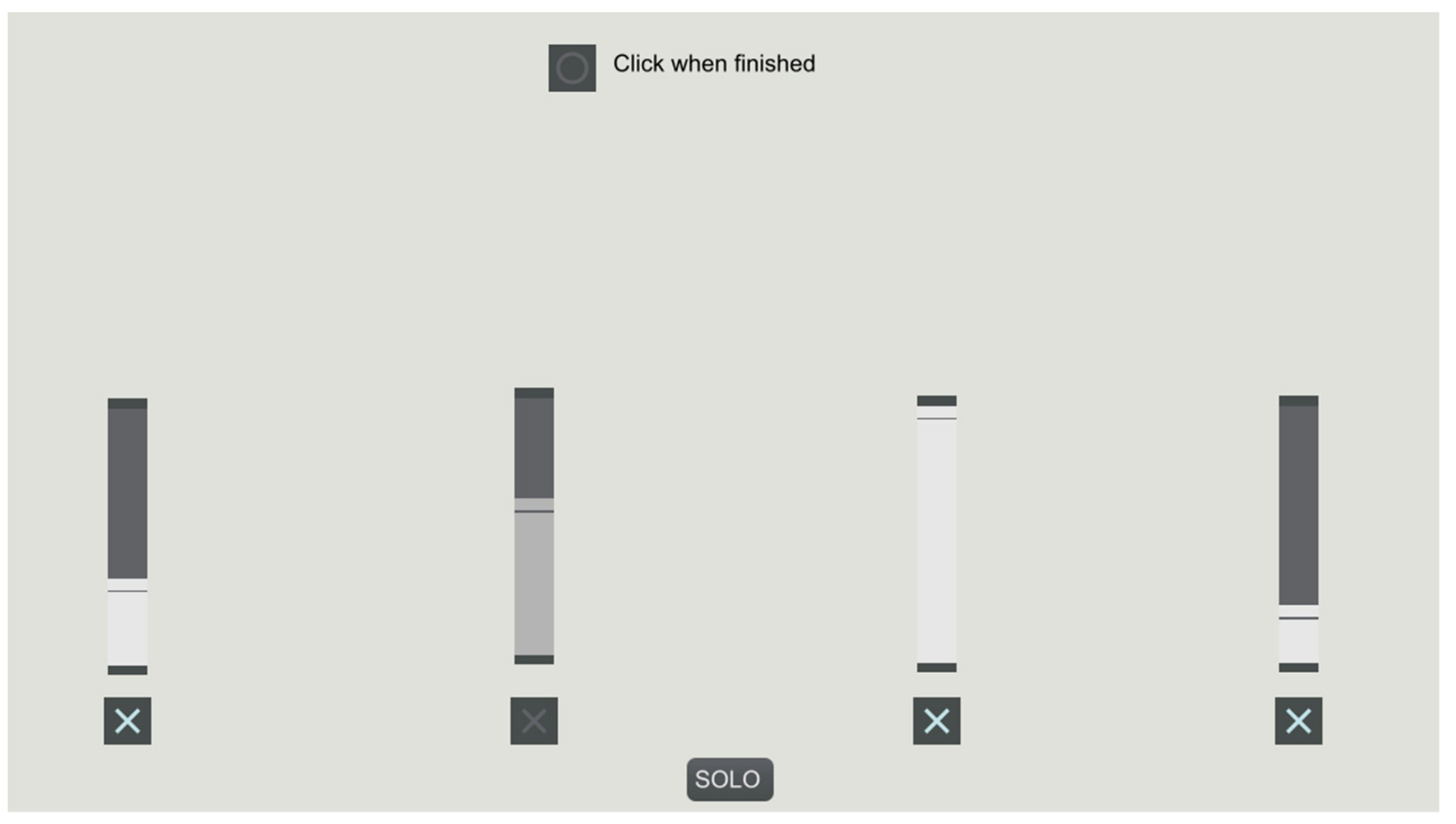
In this study, we used all but one of the same sound manipulations established in [13]. Motivations for the selected manipulations are discussed in Section 3.3. For each individual manipulation presented to the participants (Figure 1), we aimed to provide them with the means to manipulate the sounds beyond what seemed ‘useful’ in a musical context.
For example, with the distortion slider past the halfway point, the sound usually does not seem to change in any subjectively meaningful matter; the same can be said for the slope slider. This way the participants had a wide sonic range in which to explore their own perception of the use of the specific sliders. The mathematical formulations of the manipulations are now detailed.
3.1. Timbre Manipulations (FX)
3.1.1. Slope Manipulation
The amplitudes of partials are varied by a spectral “slope” manipulator α, which is used as the independent variable in experiments,
where A is the amplitude of the partial of order . If , the partials have an amplitude proportional to the inverse of their harmonic number (1, 1/2, 1/3, 1/4, etc.) approximating a sawtooth oscillation; if , all partials and have equal amplitude, approximating a pulse stream. A continuous change of α from one to zero would, therefore, have all partials continuously rising in amplitude until they are equal to A1 (the amplitude of ). This manipulation is closely related to the spectral slope audio descriptor and its linearly correlated spectral centroid audio descriptor [14].
The range given for the slope slider in the experiment was: to .
The slider manipulating the parameter had an exponentially scaled output, and the range was set to four times the range used in [13] to give the subjects a bigger range for their mix adjustments.
3.1.2. Odd to Even Ratio (OER) Manipulation
A second manipulation changes partial amplitudes, based on their harmonic number, by multiplying the amplitudes of even-number partials by the OER manipulator . The slider interface for this was flipped, however, so the slider at its minimum was , and at its maximum it was . If perfectly harmonic partials were in phase synchrony, with a slope-value of and the multiplier for even harmonics set to , the resulting sound would have no even-number harmonics and would approximate a square-wave oscillation; a similar sound but with the multiplier set to β = 1 would approximate a sawtooth oscillation. This manipulator would obviously be most closely related to the OER audio descriptor [14].
The range given for the OER slider in the experiment was: to .
This is the maximum range available for this particular manipulation. Negative values would be almost identical to their positive counterparts (only with flipped phases), and values past one (one being the same level for odd and even harmonics) would result in emphasizing a sawtooth sound an octave up with an additional sub-octave.
3.1.3. Inharmonicity Manipulation
The inharmonicity manipulator affects the frequency of the partials, based on the formula, where k is the index of the harmonic, and δ is the constant by which the ratio of harmonics is stretched or compressed. δ > 1 result in stretched partials, and δ < 1 in compressed partials. When δ = 1, the result is a perfect harmonic sound. This manipulation would be most accurately captured with the inharmonicity audio descriptor [14].
The range given for the inharmonicity slider in the experiment was: to .
This range also represents roughly double the range given in [13] with the aim of giving the subjects a bigger manipulable range for their mix adjustments.
3.1.4. Distortion Manipulation
Lastly, distortion of the signal is another variable, provided by digitally clipping the signal at fixed amplitude. For distortion, the normalized source signal amplitude is multiplied by and afterward, every value greater than one is set to one, and every signal smaller than –1 is set to –1. The effect is usually the result of increasing signal amplitude gain past the maximum capacity of any given sound system or amplifier (often referred to as “overdrive”). In digital systems, overdrive/distortion corresponds to “clipping” of the signal, which is why, within the Max/MSP 7 environment, the “clip” object was used in the signal chain to bring the signal back to ±1 so as to achieve the desired effect. Although this manipulation does not have a particular corresponding audio descriptor, it would likely affect multiple features to varying degrees (spectral flux, spectral centroid, spectral flatness, inharmonicity, spectral slope, etc.).
The range given for the distortion slider in the experiment was: to .
In [13], was set at a constant 7. With this increased range, we wanted to give the subjects the option of experimenting with a wider variety of distortion and its influence on the other parameters.
3.2. Phase and Stereo
A natural consequence of the inharmonicity manipulation is that the relative phase positions of a sound’s harmonics do not stay constant. They would instead be at unpredictable positions for most of the experiment if the inharmonicity slider was used. As established in [15], sawtooth sounds with aligned relative phase positions have a very distinct sound, whereas any other set of random phase positions of partials in complex sounds appear very similar to each other. To avoid an impact of the perfect phase sound on the starting sound settings, the partials’ phases were randomized at the start of every loop.
With the synthesizer having to be able to play two voices for the chords loop (which doubles as a sort of melody with its treble voice), this gave us the opportunity to implement stereo sounds for the bassline and arpeggio. This was accomplished by both synth voices having independent random phases and panning one voice to the left, the other one to the right while having both playing the same Musical Instrument Digital Interface (MIDI) file. This way, we were able to achieve a more realistic mixing setting, where a sound engineer would usually try to spread out the individual voices over the width of the stereo mix.
3.3. Relations of Timbre Manipulators to Physical Concepts in Music Generation
All of these manipulations or effects are common in music creation, performance, or production, as used in electroacoustic music, rock/pop, contemporary classical, or almost any other form of music. These links are briefly explained here.
3.3.1. Slope Manipulation
It is well known that the amplitudes of upper partials increase more than those for lower partials when instruments are played with a higher intensity, which makes them sound brighter [16]. In conventional synthesizers, this often leads to the velocity of the input being not only linked to the overall amplitude but also to the frequency of a cut-off filter (low-pass) to imitate the behavior of physical instruments.
3.3.2. OER Manipulation
The amplitude ratio of odd to even number harmonics has been a primary manipulator in synthesizers since the first Moogs in the sixties and seventies, where crossfading of multiple oscillators allowed for smooth variation between oscillation shapes [17]. The most common oscillation shapes in subtractive synthesis are still the sawtooth and the square wave, whose defining difference is the absence of even harmonics in the square-wave as opposed to the sawtooth-wave, which contains all the multiples of . Square waves are also closely associated with the concept of fundamental audio distortion/overdrive, which primarily adds odd harmonics. With increasing levels of overdrive or distortion, a pure sine-wave transforms into a square wave by introducing, and then continuously increasing, odd-numbered harmonics of .
3.3.3. Inharmonicity Manipulator
Many instruments produce tones with imperfectly harmonic structures. Most obviously, many percussion instruments, in particular, bells, feature large amounts of distinctly inharmonic partials and when it comes to computer music, there is no physical limit to the extent of partial detuning. But also pitched instruments, like the piano, are often characterized by the slightly detuned nature of the partials of the hammered strings [18,19], particularly the bass strings. The same goes for groups of instruments playing in unison in an orchestra or big band setting [20]. The inharmonicity manipulator serves as a general representation of this characteristic, which stretches the partials evenly along the whole spectrum by an exponential value.
3.3.4. Distortion
Whole genres of music are defined to a large extent by the nature of the distortion of the sounds (e.g., Djent, Drone-Doom, Noise, Glitch) [21,22]. The literature so far usually notes distortion simply as an effect, adding (mostly odd) harmonics to a given signal. Given that distortion/saturation/overdrive effects are amongst the most popular not only within guitar driven but also in electronic and experimental music as well as in studio production (tape saturation, microphone preamp overdrive, tube compressors, etc.), it seems to be a manipulation worth investigating. Its effect is completely dependent on the input signal, often accentuating the signal’s properties.
Applying distortion to a perfectly harmonic sound will tend to make the sound brighter and increase the amplitude of odd harmonics, and hence will be correlated with the Slope and OER manipulators. But importantly, if the input has slightly inharmonic partials, which usually is the case, it turns static signals into dynamic ones with the resulting beating (and chorusing) between the inharmonic partials of the original sound, and the new partials introduced by the distortion. Distortion is also a natural product of any physical system with a finite amplitude/pressure bandwidth, and hence it commonly arises in the real world, including the auditory system itself [23].
4. Experimental Method
For the experiment, participants (n = 28, age 18–70, median 24, male = 9, female = 18, other = 1, Goldsmith Music Sophistication Index (GMSI) 31–117, median 75, no professional sound engineers or music producers) were instructed to manipulate a series of musical loops, examples being available online, via a set of four sliders on a laptop in front of them. The loops, which played alongside a premade drum loop, were designed to roughly represent a prototype of a “Bassline”, a “Harmony”, which would also double as a type of melody, and an “Arpeggio”, another type of melody, of a musical piece section. These loops were presented over headphones (Audio-Technica M50x) by the same laptop. A participant’s task was to make the loop sound as good as possible to him or her, given their ability and preference. For this setup, an additive synthesizer was created in Max/MSP that was able to generate sounds consisting of a fundamental frequency and up to 275 harmonics. The harmonics were manipulable according to the FX established in Section 5. This synthesizer was able to play simple MIDI files in a loop and then record the resulting output into an audio file (44.1kHz/16bit, *.wav). Accompanying the MIDI loop was an audio loop with a pre-recorded drumbeat to give a more realistic musical context.
Although adjusting the volume of the individual voices is usually one of the core aspects of music mixing, this option was purposely not given to the participants. Since the focus of this study was on timbre, with 50% of its entire definition being “aspects of a sound, which are not loudness”, it would have been counterproductive to the aim of the experiment. Additionally, since louder sounds are generally preferred by listeners [24], a novice mixer often only increases the volume of all the voices, not paying attention to their timbre, ending up with just an overall louder mix.
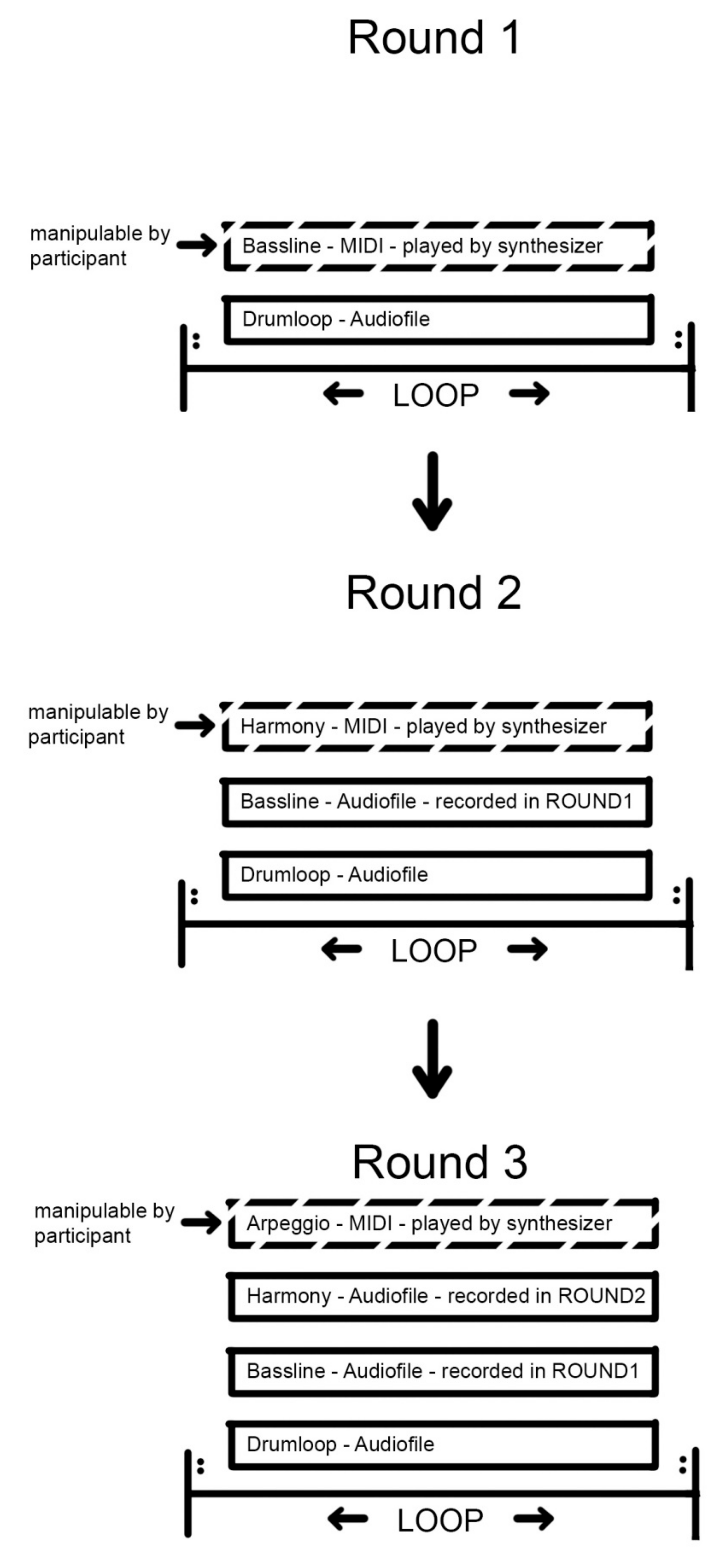
First, the participant adjusted the sound of the bassline, accompanied by the unchanging drum pattern. When the participant was satisfied with the result of their slider settings for the first “bassline” loop, they could click on a “continue” button, which caused the synthesizer to play through the loop once more and record the output into a separate audio file. In the next step, a second MIDI loop “harmony” would start to be played by the synthesizer, again manipulable by the four sliders. From the second repetition onwards, this MIDI loop was accompanied by the recorded audio of the “bassline” first loop. Again, the participant could mix this loop and record it to the computer when finished, which would trigger the third iteration of this process, now with the “arpeggio” loop, accompanied by both, bassline and harmony loops, as well as the drum loop. The process is visualized in Figure 2.
This order of musical phrases was chosen to represent a common bottom-up mixing strategy in pop music, where an audio engineer would often mix in this order: that is, Drums, Bass, guitars/synths, vocals, and finally any extras. After this last loop, the entire process would start anew with a second set of looped phrases, until the participant had mixed a total of five looped musical pieces (although each such musical piece is only eight or sixteen bars). During the mixing phases, the participant was given the option of muting all the other audio loops with a “SOLO” button, singling out the presently manipulable MIDI loop, for a clearer understanding of the changes effected by the sliders on that musical phrase. The muted tracks could be unmuted with a “FullMix” button, which appeared instead of the “SOLO” button, when solo-mode was engaged. Whenever the participant was finished with mixing a phrase and clicked “continue”, the final positions of the sliders for the given loop were recorded, as was the musical loop itself.
To minimize effects of perceived loudness, first, a routine was implemented to keep the Root-Mean-Square (RMS) level of the individual played loop constant over changes to the FX. Second, a moderate dynamic volume adjustment was implemented, which adjusted the synth level based on the measured spectral centroid of the synthesizer’s output and a weighting based on the Equal Loudness Contour as described in ISO 226 [25]. In this way, we tried to partially compensate for the human ear frequency response. Additionally, to replicate a key aspect of the modern day mixing and mastering, mild “ducking” of the audio and MIDI tracks were implemented, triggered by the accompanying drum loop. In the present case, this means a dynamic lowering of the synth and audio track amplitude, based on the RMS amplitude of the drum loop (set at very short 0.45 ms attack and release).
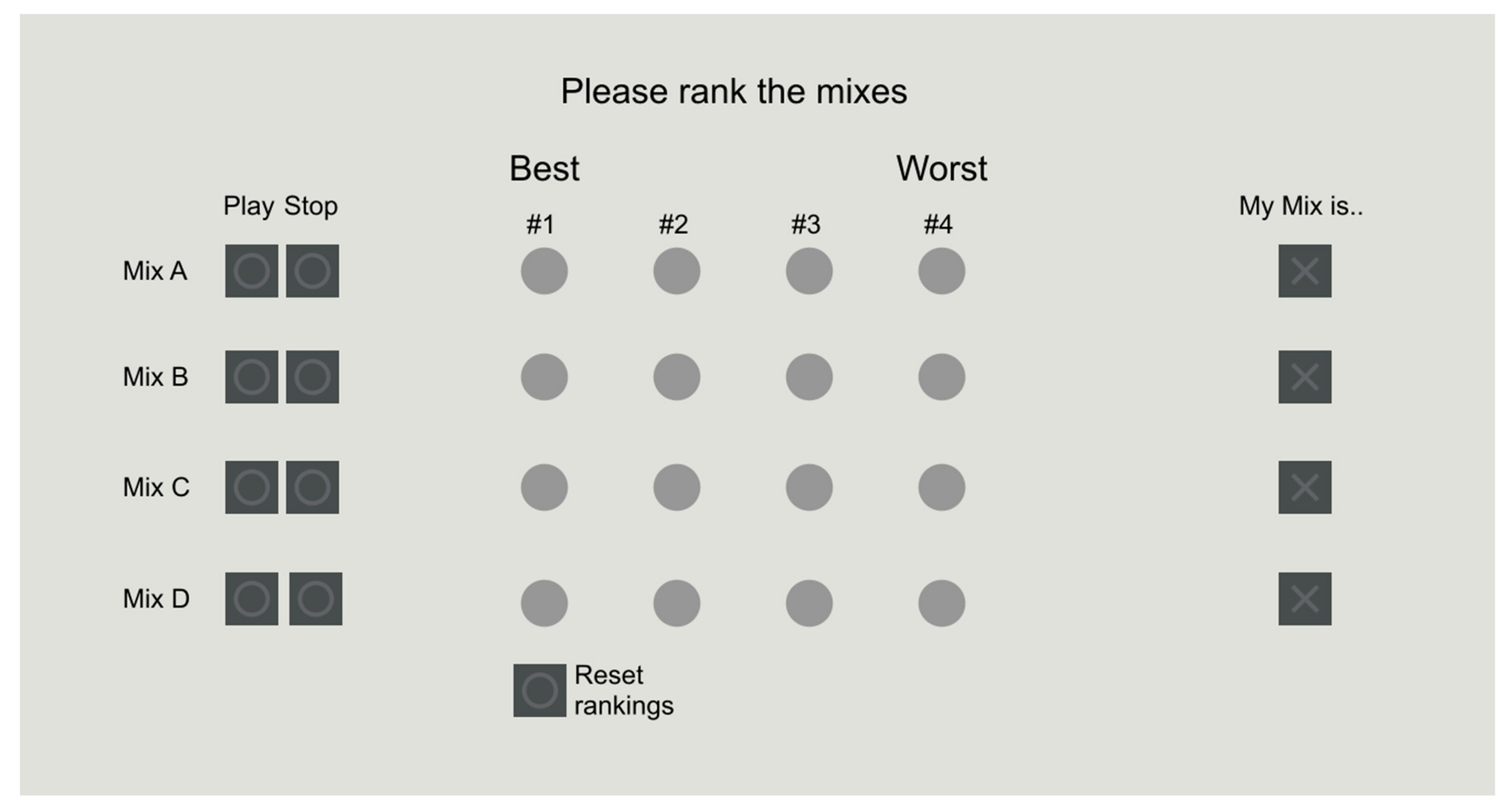
In the second part of the experiment, the participant was asked to rank four different mixes of each of the same five musical pieces according to their liking (Figure 3). Only one was from the current participant. For this, the participant was presented with “play” and “stop” buttons for four mixes, titled Mix A, B, C, and D. The play button would start the combination of the three loops of a specific mix to be played in a loop until the stop button was pressed. In five button matrix (four mixes, four ranks), the participant could then assign #1–#4 in order of preference to the mixes (#1 being best, #4 being worst), with no option of two or more mixes being the same rank for all five musical pieces. Additionally, the participant was asked to indicate via a tick box which of the mixes they thought was their own.
In this manner, the participant was asked to rank mixes of all five previously mixed musical pieces. The order of mixes behind A, B, C, D was always randomized, but they represented the mix as mixed by the participant (P-Mix), a mix (E-Mix) as mixed by an expert audio engineer (Bachelor’s Degree in Audio Engineering, Master’s Degree in Classical Music, professionally working in music recording, -mixing, -mastering, also first author of this paper), a mix with all sliders set to zero, resulting in sawtooth oscillation (S-Mix), and a mix with all sliders at random positions (R-Mix: to prevent all participants ranking just one specific random mix, which might turn out particularly bad or good, instead a pool of 50 different fixed random mixes was generated with each participant receiving a different one). Examples for the sawtooth and expert mixes of the five musical pieces can be found in the Supplementary Materials.
After the ranking of the mixes, the participant was asked to complete a survey, asking about general background information, as well as the self-reporting part of the Goldsmith Music Sophistication Index (GMSI) survey. Additionally, the participants were directly asked four questions about their approach to the experiment:
- “Did you think you succeeded in improving the mixes towards your taste?”
- “Did you predominantly use SOLO or FullMix mode, or a mixture of both?”
- “Did you have a specific mixing strategy or goal in mind?”
- “Was there a kind of sound manipulation method you were missing?”
4.1. The Musical Pieces
The first musical piece was composed by the first author to represent a simple and common pop chord progression (B-minor | E7 | B-minor | A7), accompanied by a 16th-note groove in the drumbeat on a medium fast tempo of 140 bpm.
The second musical piece was composed by the first author with an intent to roughly represent the aesthetics of a Drum’n’Bass track. It had a relatively fast 8th-note beat at 165 bpm with a lesser emphasis on beat two and four and a bassline that incorporated a lot of movement both in terms of rhythmic variation and pitch height of fundamental frequency.
The third musical piece was a synth adaption of a track by emerging Sydney progressive rock unit “Illusion of Grandeur”. It represented six bars of a slower rock track in 3/4, with a tempo of 80 bpm, frequent irregular drum fills on toms, and a minor focused chord progression of F-minor | Db-major | Bb-minor.
The fourth musical piece was designed to mimic the instrumental part of a hip-hop track. It consisted of a mid-tempo 96 bpm 8th-note drumbeat with a heavy emphasis on beats two and four and a simple chord progression (G#minor | Gmajor | D#7/A# | A7) with chromatic melodic elements.
Track number five was designed as a control to consist of the same elements as the previous tracks but to have no recognizable musical intent. To this end, the drum loop, as well as the pitched MIDI loops, were created by semi-randomly clicking notes into the music sequencer software, but still maintaining some basic characteristics of the designated loop (bassline lower in register than harmony/arpeggio, arpeggio being continuous and having consistent arpeggio pattern, harmony having two voices).
Sound samples of the musical pieces are provided in the online Supplementary Materials.
5. Data Analysis
To model the influence of the different mixes on the mix-rankings, we used a Bayesian ordinal mixed-effects regression model (a weakly informative student t-distribution prior with three degrees of freedom, centered at zero, scale set to 2.5, was applied to all population-level effects) with the brms package [26] of the R statistics software (version 3.5.0). The ranking was defined as the response variable; the population levels effects were Mix type (P-Mix, E-Mix, S-Mix, and R-Mix), MyMix (a binary variable, indicating if the mix was marked as the participants own mix), and musician status (reflected in the Goldsmiths Musical Sophistication Index, GMSI; and these were also allowed to vary across different musical pieces and subjects as group-level effects (population-level and group-level effects are analogous to the fixed and random effects used in a classical frequentist, non-Bayesian statistical framework)). To calculate evidence for preferences for mix types, this was followed by a hypothesis testing for the coefficient of the Bayesian model for each of the mixes being either smaller or greater than zero for any given comparison mix.
To perform cluster analysis on the slider settings for the synthesizer by the participants, all sliders were normalized and then z-scores were calculated by the standard deviation of the specific slider per participant, centered on zero. A silhouette plot of the k-means clustering of the dataset in Matlab 2014 shows segmentation into two clusters having the highest silhouette mean-value of 0.69, indicating a fairly clear-cut clustering (silhouette values can range from −1 to 1).
To assess the similarity between participants’ approaches to the mixes, we split the standardized slider data by participants and correlated the data vectors to generate a correlation matrix. To gain insight into the similarity of mixing approaches, we did the same thing on the data split by musical piece to generate five vectors to get a matrix for the musical pieces.
6. Results
6.1. Mix Type Preferences
Table 1 shows that participants rank their personal mixes better than a random, expert, or sawtooth mixes. There is also strong evidence that random and expert mixes are preferred over the sawtooth mix; however, there was no evidence for preference between the random and the expert mixes.
Also, as seen in Table 2, participants tend to have a strong preference for mixes, which they indicate as their own (regardless of whether it is true or not).
When identifying their own mixes, participants were right only 28% of the time. Given the four choices, this is similar to a chance level. The proportion of mixes being indicated as their own is shown in Table 3.
6.2. Participant Correlations and Clustering
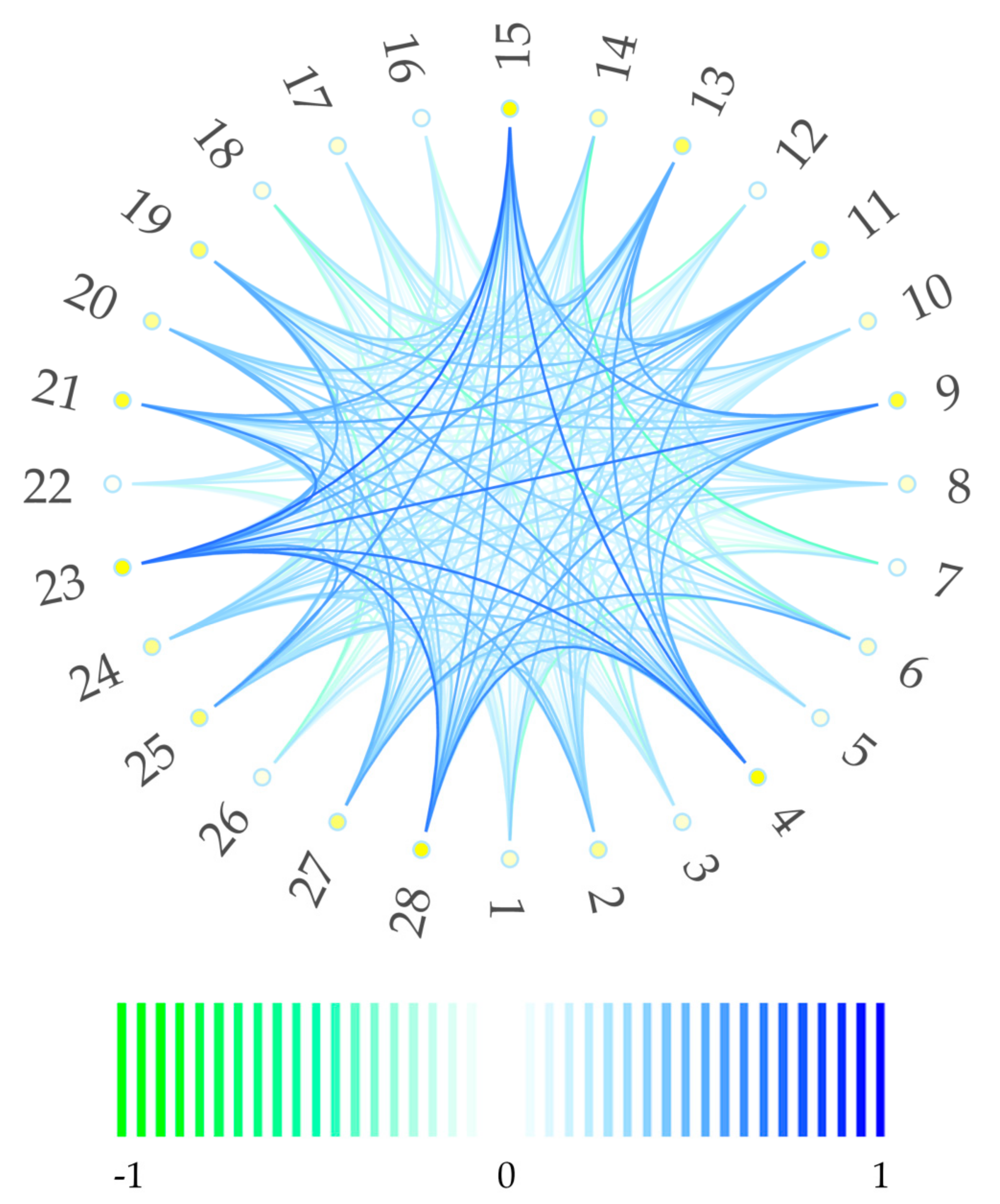
The correlations between the participants in their mixing behavior, as illustrated in Figure 4, shows a small group of highly correlated participants (4, 9, 15, 23, 28, and to a lower degree 11, 13, 19, 20, 25, 27) and a large group of other participants behaving independently to those two groups and each other. The correlations go as high as 0.74 for some of the participants.
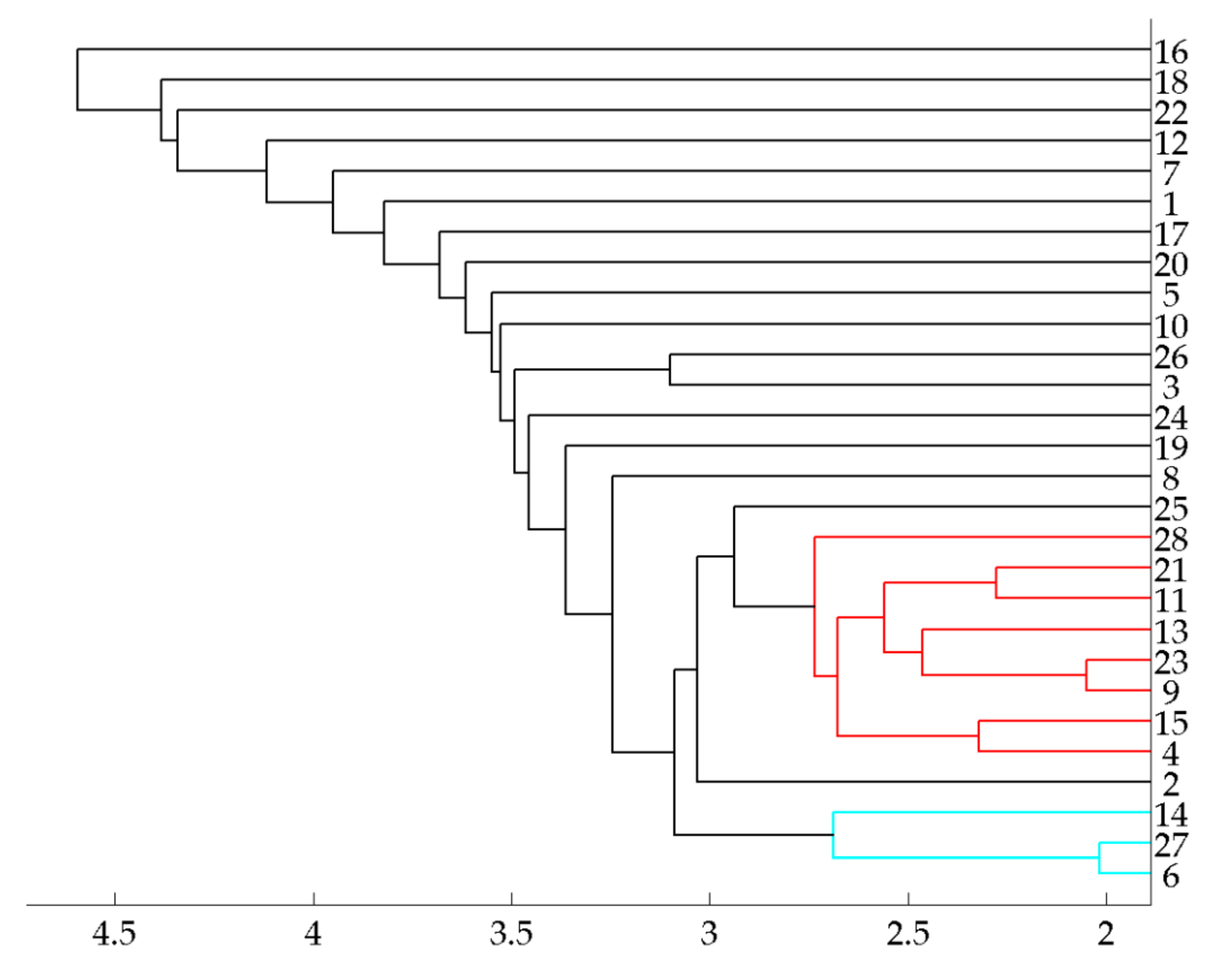
A hierarchical clustering of the same data (divided by participants), done with the linkage and dendrogram functions of Matlab 2014, shows a similar result (Figure 5), but identifies two groups of participants clustering with shorter data point distances (6, 27, 14 and 4, 15, 9, 23, 13, 11, 21, 28) and the larger group of other participants further apart.
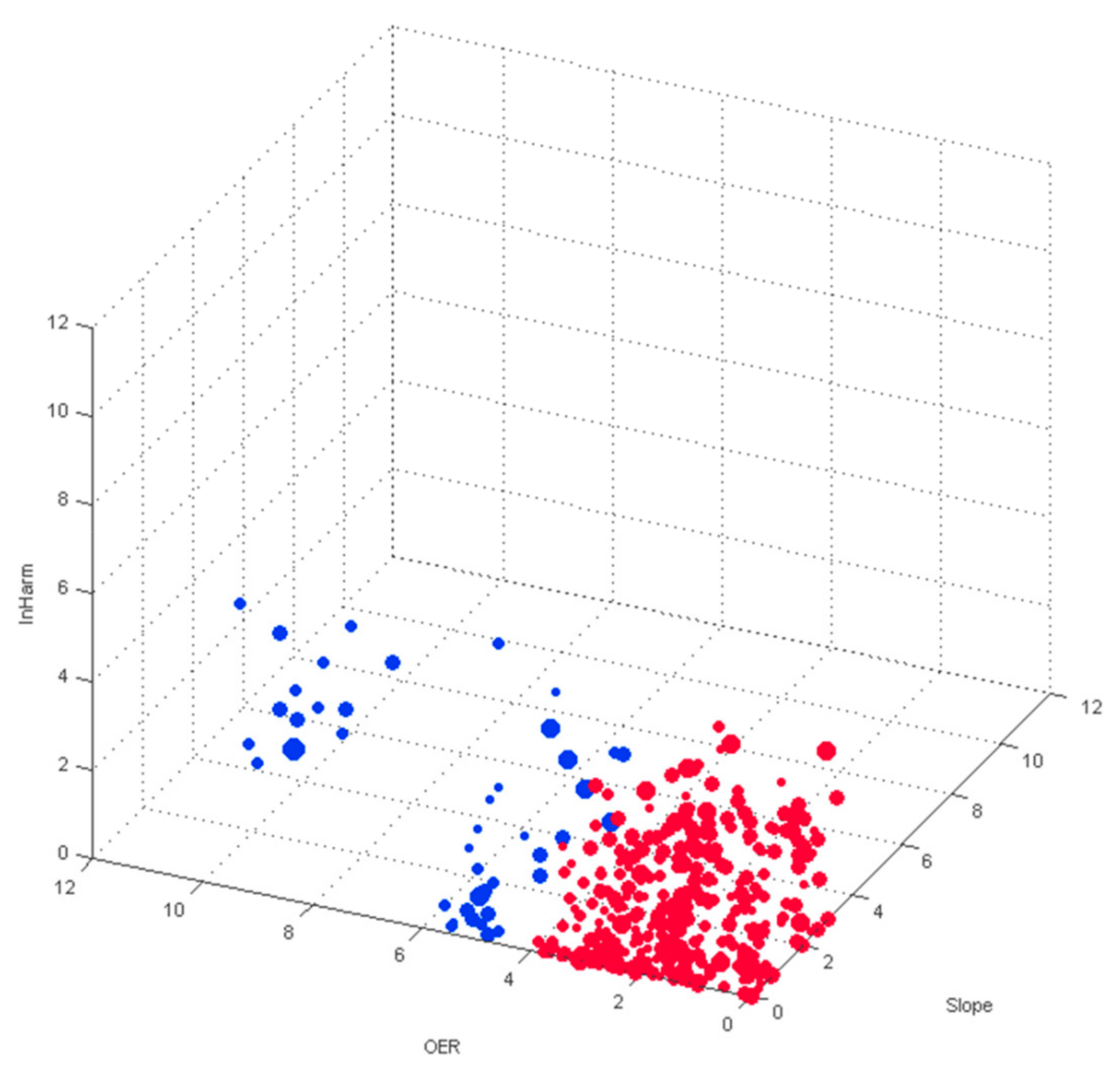
A k-means cluster analysis of the slider data was conducted to find specific mixing clusters that might arise. The result shows the silhouette value for a clustering into two groups being highest. Plotting all slider settings in a 4-D space and splitting into the two clusters in Figure 6 suggest the OER value to be the primary deciding factor between the two groups.
In the post-task questions, all of the participants, save for one, indicated thinking to have been able to improve on the mixes at least to some degree. Most of them used a mixture of “SOLO” and “FullMix” modes. They usually utilized either no particular mixing strategy or a variety of different ones. Participants either tried to eliminate unpleasant parts of the sound to adjust the level of sounds by timbral means or to overall improve “clarity”, although some answers are difficult to interpret (“[…] the strategy was P H A T, with a capital P!”).
7. Discussion and Conclusions
The results from the Bayesian model of the mix ratings show that participants generally prefer their own mixes over the others and also display a significantly lower ranking of the unmixed sawtooth mix. Also, as shown in Table 2, participants seem to expect to like their mix better than others, independent of whether they correctly identify their own mix, which, in general, they did not. An interesting sidenote to this is, as shown in the cluster analysis and the correlations of participants: the individual mix approaches seem to differ considerably for a majority of participants, but still lead to participants generally preferring their own mix. This confirms parts of [13], where experienced audio engineers would consistently rate their own mixes best. This finding seems to translate to novice engineers as well, who demonstrably are not able to recognize their own mix. This implies that listeners’ preferences are relatively individual and consistently preferred to an expert’s attempt. With regard to the initially stated aim of investigating which particular mixing choices would inform preference ratings, the conclusion would, therefore, be a “no consensus”. It might also indicate that, in this case, our expert was just particularly bad at the job.
Musical sophistication turned out to be a strong predictor only in the case of interaction with rankings for MixS (Estimate: −0.56, Evidence Ratio = 32.06), indicating participants with higher musical sophistication disliked the starting sawtooth mix slightly less than those with lower musical sophistication. At the present time, we have no explanation for this.
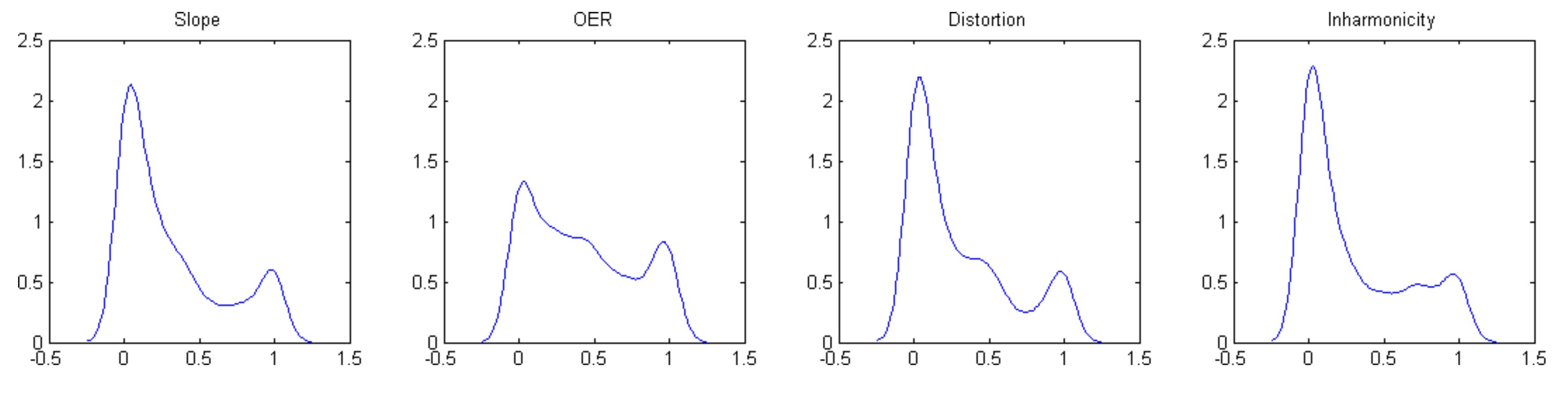
A look at a probability density function plot for the sliders (Figure 7) seems to imply a common archetype for the synth settings, with slope, distortion, and harmonicity close to zero and OER mainly close to zero or close to one; however, this archetype then would roughly approximate the sawtooth sound (for OER set at 0) or a square wave sound (for OER set at one), the former being generally ranked as the least favorite of the mixes. The implication would be that even tiny deviations from the sawtooth sound go a long way in terms of transforming timbral liking.
To get a better understanding of these ‘tiny deviations’, we expressed the median of the participants’ synth settings in units of Perception Threshold (PT: as established in [13]). These represent the amount of timbral change in units of minimum perceivable change, expressing the slider settings in a quasi-comparable distance of perceived change. The units used represent the average PT over the three originally tested F1 (80 Hz, 240 Hz, and 600 Hz) for the FX starting values of zero, Slope, OER, and Distorted Inharmonicity. Since distortion was a set value in the original paper, no unit could be attached to the slider from this experiment, but since distortion was used in 84% of melodies, and the average amount of distortion used was even higher than the amount used in [13], distorted inharmonicity was used as the PT Unit for the inharmonicity manipulation. Displaying the remaining values’ median in their corresponding PT gives the following list (Table 4).
Given the nature of the OER manipulation, with the even harmonics ranging from a minimum of not present to a maximum of equal amplitude to odd harmonics, the perceptual range of this specific manipulation can only have a maximum perceptual distance of 7.3 PT. Out of those three manipulations, the OER, therefore, apparently would have the least perceptual impact, an impact that arguably decreases even further with higher values of slope or distortion. The probability density function, shown in Figure 7, also suggests a substantial impact of the user interface on the final settings of this slider: all of the sliders have local maxima at their maximum and minimum settings, with most sliders having a pronounced one at the minimum, but OER actually has fairly equal maxima at both extremes (the median PT for the low and high halves of the OER settings are 1.84 and 5.4, respectively).
Despite multiple statements from participants about difficulties with the inharmonicity manipulation (“only used 4th slider, if the sound was high pitched”, “I wanted to make ‘smoother’ sounds, did not like the 4th slider, very inharmonious!”, “alien-slider (4) was fun, but I didn’t use it much”, etc...), according to the median PT of the slider settings, the most perceptually relevant timbral change was apparently induced by it. This is despite the fact that the harmonicity slider actually being left at its zero position most often out of the four (see Table 5). The main timbral change was achieved predominantly with drastic changes in inharmonicity (in relation to its PT) compared with the changes used in the other sliders.
A notable restriction to the usage of PT is that the given values theoretically only represent the given value from the zero position of their slider, with all other sliders being set at zero as well, so they only ever represent a rough estimate. This means that the PT expression of the median values can only represent the perceptual distance from the starting sound (the sawtooth). Secondly, the perceptual impact of, for example, inharmonicity would most likely be reduced for higher settings of slope due to the higher partials, which are affected by the inharmonicity slider, being attenuated by the slope manipulation.
Regarding the clustering of the mixing settings, the perceptual impact of OER also contextualizes the results of the k-means/silhouette readings of the slider data. The clustering seems to indicate two strong clusters, which are predominantly characterized by their OER value, something that looks equally convincing in Figure 7. To test whether this binary split of the OER settings represents two distinct mixing clusters, a mixed effects model was run in R, with the OER settings (rounded to either zero or one) as the response variable, slider settings for Slope, Distortion, and Inharmonicity as fixed effects, and participant id as random effects. This did not show any power of the other sliders in predicting OER, implying that there is no distinct grouping of the other settings related to the chosen OER values. This in combination with the low perceptual impact of OER supports the suggestion that the distinct clustering in the k-means analysis is predominantly due to the affordances of the user interface (UI). Alternatively, it could be interpreted as there is a preference for those two extremes over more middling values since 7.9 PTs of the range should still be clearly audible, but the effect is still subtle; hence participants chose the extremes because intermediate settings were less distinct.
7.1. Future Work
With the present study suggesting listeners prefer their own mixes, an interesting follow-up would be to determine whether such preferences for their mixes apply also to new (inexpert) listeners when rating them. With new participants, perhaps the expert mix might be given time to shine when compared to the previous participant mixes by a new group of inexpert listeners. Additionally, it would make sense to incorporate multiple experts’ mixes in a study. To this end, a study that asks participants to rank random mixes, expert mixes, novice mixes, and the sawtooth mix would reveal whether experts might still have a “leg up” on novices in their own field. Furthermore, this would show whether the mixes of the group of novices, which showed a high correlation in their mix approaches in the circular diagram and the hierarchical clustering, stand out in any way. If there are mixes with significantly higher ratings in this approach, following up with a spectral feature analysis of these specific mixes might reveal underlying audio features for these preferences. Possibly, the preferences of expert audio mixing engineers could be tuned more fully to those of their (necessarily largely inexpert) audience.
Supplementary Materials
The following are available online at https://0-www-mdpi-com.brum.beds.ac.uk/2076-3417/9/8/1695/s1, Audio S1: Song01—MixS, Audio S2: Song01—MixE, Audio S3: Song02—MixS, Audio S4: Song02—MixE, Audio S5: Song03—MixS, Audio S6: Song03—MixE, Audio S7: Song04—MixS, Audio S8: Song04—MixE, Audio S9: Song05—MixS, Audio S10: Song05—MixE.
Author Contributions
Conceptualization, F.A.D., A.J.M., and R.T.D.; methodology, F.A.D., A.J.M., and R.T.D.; software, F.A.D.; validation, A.J.M. and R.T.D.; formal analysis, F.A.D.; investigation, F.A.D.; data curation, F.A.D.; writing—original draft preparation, F.A.D.; writing—review and editing, A.J.M. and R.T.D.; visualization, F.A.D.; supervision, A.J.M. and R.T.D.; project administration, F.A.D.
Funding
This research received no external funding.
Acknowledgments
We would like to acknowledge Steffen A. Herff for additional critical review on later drafts of the manuscript.
Conflicts of Interest
The authors declare no conflict of interest.
References
- Wishart, T. Audible Design: A Plain and Easy Introduction to Practical Sound Composition; Orpheus The Pantomime: York, UK, 1994. [Google Scholar]
- Bregman, A.S. Auditory Scene Analysis: The Perceptual Organization of Sound; MIT Press: Cambridge, MA, USA, 1994. [Google Scholar]
- Martin, K.D. Sound-Source Recognition: A Theory and Computational Model. Ph.D. Thesis, Massachusetts Institute of Technology, Cambridge, MA, USA, 1999. [Google Scholar]
- Fung, C.V. Musicians’ and Nonmusicians’ Preferences for World Musics: Relation to Musical Characteristics and Familiarity. J. Res. Music Educ. 1996, 44, 60–83. [Google Scholar] [CrossRef]
- Saldanha, E.L.; Corso, J.F. Timbre Cues and the Identification of Musical Instruments. J. Acoust. Soc. Am. 1964, 36, 2021–2026. [Google Scholar] [CrossRef]
- Agostini, G.; Longari, M.; Pollastri, E. Musical Instrument Timbres Classification with Spectral Features. EURASIP J. Adv. Signal Process. 2003, 2003, 943279. [Google Scholar] [CrossRef]
- McAdams, S.; Giordano, B.L. The Perception of Musical Timbre. In The Oxford Handbook of Music Psychology; Oxford University Press: Oxford, UK, 2009; pp. 72–80. [Google Scholar]
- Hailstone, J.C.; Omar, R.; Henley, S.M.D.; Frost, C.; Kenward, M.G.; Warren, J.D. It’s Not What You Play, It’s How You Play It: Timbre Affects Perception of Emotion in Music. Q. J. Exp. Psychol. 2009, 62, 2141–2155. [Google Scholar] [CrossRef] [PubMed]
- Aucouturier, J.-J.; Pachet, F.; Sandler, Ma. “The Way It Sounds”: Timbre Models for Analysis and Retrieval of Music Signals. IEEE Trans. Multimed. 2005, 7, 1028–1035. [Google Scholar] [CrossRef]
- Fortney, P.M.; Boyle, J.D.; DeCarbo, N.J. A Study of Middle School Band Students’ Instrument Choices. J. Res. Music Educ. 1993, 41, 28–39. [Google Scholar] [CrossRef]
- Delzell, J.K.; Leppla, D.A. Gender Association of Musical Instruments and Preferences of Fourth-Grade Students for Selected Instruments. J. Res. Music Educ. 1992, 40, 93–103. [Google Scholar] [CrossRef]
- De Man, B.; Boerum, M.; Leonard, B.; King, R.; Massenburg, G.; Reiss, J.D. Perceptual Evaluation of Music Mixing Practices. Paper presented at the 138th Audio Engineering Society Convention, Warsaw, Poland, 7–10 May 2015. [Google Scholar]
- Dobrowohl, F.A.; Milne, A.J.; Dean, R.T. Controlling Perception Thresholds for Changing Timbres in Continuous Sounds. Organ. Sound 2019, 24. in press. [Google Scholar]
- Peeters, G.; Giordano, B.L.; Susini, P.; Misdariis, N.; McAdams, S. The Timbre Toolbox: Extracting Audio Descriptors from Musical Signals. J. Acoust. Soc. Am. 2011, 130, 2902–2916. [Google Scholar] [CrossRef] [PubMed]
- Laitinen, M.-V.; Disch, S.; Pulkki, V. Sensitivity of Human Hearing to Changes in Phase Spectrum. J. Audio Eng. Soc. 2013, 61, 860–877. [Google Scholar]
- Dannenberg, R.B.; Derenyi, I. Combining Instrument and Performance Models for High-Quality Music Synthesis. J. New Music Res. 1998, 27, 211–238. [Google Scholar] [CrossRef]
- Moog, R.A. Electronic Music Synthesizer. U.S. Patents US 4,050,343, 27 September 1977. [Google Scholar]
- Järveläinen, H.; Välimäki, V.; Karjalainen, M. Audibility of Inharmonicity in String Instrument Sounds, and Implications to Digital Sound Synthesis. Paper presented at the ICMC, Beijing, China, 22–27 October 1999. [Google Scholar]
- Schuck, O.H. Observations on the Vibrations of Piano Strings. J. Acoust. Soc. Am. 1943, 15, 1–11. [Google Scholar] [CrossRef]
- Cohen, E.A. Some Effects of Inharmonic Partials on Interval Perception. Music Percept. Interdiscip. J. 1984, 1, 323–349. [Google Scholar] [CrossRef]
- Berger, H.M.; Fales, C. “Heaviness” in the Perception of Heavy Metal Guitar Timbres. In Wired for Sound: Engineering and Technologies in Sonic Cultures; Wesleyan University Press: Middletown, CT, USA, 2010; pp. 181–197. [Google Scholar]
- Van Nort, D. Noise/Music and Representation Systems. Organ. Sound 2006, 11, 173–178. [Google Scholar] [CrossRef]
- Lee, K.M.; Skoe, E.; Kraus, N.; Ashley, R. Selective Subcortical Enhancement of Musical Intervals in Musicians. J. Neurosci. 2009, 29, 5832–5840. [Google Scholar] [CrossRef] [PubMed] [Green Version]
- Cullari, S.; Semanchick, O. Music Preferences and Perception of Loudness. Percept. Motor Skills 1989, 68, 186. [Google Scholar] [CrossRef] [PubMed]
- ISO BS. 226:2003: Acoustics-Normal Equal-Loudness-Level Contours; International Organization for Standardization: Geneva, Switzerland, 2003. [Google Scholar]
- Bürkner, P.-C. Brms: An R Package for Bayesian Multilevel Models Using Stan. J. Stat. Softw. 2016, 80, 1–28. [Google Scholar] [CrossRef]
- Kruschke, J.K. Rejecting or Accepting Parameter Values in Bayesian Estimation. Adv. Methods Pract. Psychol. Sci. 2018, 1, 270–280. [Google Scholar] [CrossRef] [Green Version]
Figure 1.
Screenshot of the mixing interface. Sliders from left to right were affecting Slope, OER (odd/even ratio), Distortion, Inharmonicity. The ‘X’ buttons below the sliders toggle the sliders’ output between zero and its’ set value for an easy A/B comparison to the start setting.
Figure 1.
Screenshot of the mixing interface. Sliders from left to right were affecting Slope, OER (odd/even ratio), Distortion, Inharmonicity. The ‘X’ buttons below the sliders toggle the sliders’ output between zero and its’ set value for an easy A/B comparison to the start setting.

Figure 2.
Representation of the process of part one of the experiment. MIDI = Musical Instrument Digital Interface.
Figure 2.
Representation of the process of part one of the experiment. MIDI = Musical Instrument Digital Interface.

Figure 3.
Screenshot of ranking interface for a single musical piece.

Figure 4.
Schemaball illustration of Pearson correlations between participants. The numbers around the circle represent the participants, the color of the connecting lines (green to white to blue) represents the coefficient, and the color of the dots next to the number represents the average coefficient of the participant.

Figure 5.
Dendogram of hierarchical clustering of participants; the x-axis represents the relative distance of individual participants, with the color cut-off being 60% of the biggest distance.
Figure 5.
Dendogram of hierarchical clustering of participants; the x-axis represents the relative distance of individual participants, with the color cut-off being 60% of the biggest distance.

Figure 6.
Scatterplot, with the “Distortion” settings being displayed as the dot size. Colors indicate the two different clusters as calculated by the k-means analysis. All displayed values are z-scores as distance in standard deviations (per participant) from zero.
Figure 6.
Scatterplot, with the “Distortion” settings being displayed as the dot size. Colors indicate the two different clusters as calculated by the k-means analysis. All displayed values are z-scores as distance in standard deviations (per participant) from zero.

Figure 7.
Probability density plot of slider distributions, X = Slider Value, Y = Probability density estimate. The bandwidth of the kernel smoothing window = 0.08. OER = odd/even ratio.
Figure 7.
Probability density plot of slider distributions, X = Slider Value, Y = Probability density estimate. The bandwidth of the kernel smoothing window = 0.08. OER = odd/even ratio.


Table 1.
The output of the hypothesis testing for values of the coefficients of the Bayesian model is greater or smaller than 0 for any given reference mix. An Evidence Ratio of 3–10 indicates “substantial” evidence for the reported observation; Evidence Ratios of 10+ indicate strong evidence for the observation [27]. Since lower numbers for rank indicate a greater preference, negative coefficients in the “estimate” column indicate a preference for the tested mix, and positive ones indicate a preference for the reference mix. Reported are results with evidence ratio ≥3. MixS = Sawtooth Mix, MixP = Personal Mix, MixE = Expert Mix, MixR = Random Mix, CI—Confidence Interval.
| Hypothesis | Estimate | Est.Error | CI.Lower | CI.Upper | Evid.Ratio | Reference Mix |
|---|---|---|---|---|---|---|
| MixS > 0 | 0.36 | 0.21 | 0.0 | Inf | 19.51 | Random |
| MixP < 0 | −0.23 | 0.21 | −Inf | 0.11 | 6.34 | Random |
| MixS > 0 | 0.31 | 0.22 | −0.04 | Inf | 13.18 | Expert |
| MixP < 0 | −0.28 | 0.22 | −Inf | 0.07 | 9.1 | Expert |
| MixE < 0 | −0.3 | 0.22 | −Inf | 0.06 | 10.66 | Saw |
| MixR < 0 | −0.35 | 0.22 | −Inf | 0.01 | 16.78 | Saw |
| MixP < 0 | −0.59 | 0.22 | −Inf | −0.24 | 499 | Saw |
| MixS > 0 | 0.59 | 0.22 | 0.24 | Inf | 332.33 | Personal |
| MixE > 0 | 0.28 | 0.22 | −0.08 | Inf | 8.93 | Personal |
| MixR > 0 | 0.23 | 0.22 | −0.14 | Inf | 6.18 | Personal |
Table 2.
The output of the Bayesian model with MixS as the reference level. The Estimate is the mean of each effect’s posterior distribution, l–95% and u–95% are the lower and upper bounds of the effects’ 95% credibility interval (the data tell us that the effect’s true size has a 95% probability of falling in this interval), respectively. If the 95% CI (Confidence Interval) does not cross zero, the effect can be considered “significant”. MixY:GMSI effects are the interaction effects between Goldsmith Music Sophistication Index (GMSI) and the specified mix ratings. MixS = Sawtooth Mix, MixP = Personal Mix, MixE = Expert Mix, MixR = Random Mix.Population-Level Effects.
| Effect | Estimate | Est.Error | l–95% CI | u–95% CI |
|---|---|---|---|---|
| MixE | −0.3 | 0.22 | −0.74 | 0.13 |
| MixR | −0.35 | 0.22 | −0.77 | 0.08 |
| MixP | −0.59 | 0.22 | −1.01 | −0.16 |
| MyMix | −0.95 | 0.18 | −1.31 | −0.58 |
| MixS:GMSI | −0.53 | 0.3 | −1.12 | 0.07 |
| MixE:GMSI | −0.32 | 0.29 | −0.88 | 0.25 |
| MixR:GMSI | 0.16 | 0.32 | −0.47 | 0.78 |
| MixP:GMSI | −0.05 | 0.30 | −0.64 | 0.54 |
Table 3.
Percentage of mixes being identified as the participants own.
| Mix | Identified as Own |
|---|---|
| Personal: | 28% |
| Random: | 17% |
| Sawtooth: | 25% |
| Expert: | 30% |
Table 4.
Median slider setting in units of PT (Perception Threshold). In the special bi-modal case of OER (odd/even ratio), the median PT values for the slider range 0.0–0.5 and 0.5–1.0 are 2.05 and 5.91, respectively. FX = timbre manipulations.
Table 4.
Median slider setting in units of PT (Perception Threshold). In the special bi-modal case of OER (odd/even ratio), the median PT values for the slider range 0.0–0.5 and 0.5–1.0 are 2.05 and 5.91, respectively. FX = timbre manipulations.
| FX | Median PT | Slider Range in PT |
|---|---|---|
| Slope | 21.04 | 145.5 |
| OER | 4.63 | 7.3 |
| Inharmonicity | 219.67 | 1550.0 |
Table 5.
Percentages of individual sliders being left at their starting (zero-) positions. OER = odd/even ratio, FX = timbre manipulations.
Table 5.
Percentages of individual sliders being left at their starting (zero-) positions. OER = odd/even ratio, FX = timbre manipulations.
| FX | % of Manipulation Being Left at 0-Value |
|---|---|
| Slope: | 9.28% |
| OER: | 20.24% |
| Distortion: | 16.19% |
| Inharmonicity: | 30.23% |
© 2019 by the authors. Licensee MDPI, Basel, Switzerland. This article is an open access article distributed under the terms and conditions of the Creative Commons Attribution (CC BY) license (http://creativecommons.org/licenses/by/4.0/).
Share and Cite
MDPI and ACS Style
Dobrowohl, F.A.; Milne, A.J.; Dean, R.T. Timbre Preferences in the Context of Mixing Music. Appl. Sci. 2019, 9, 1695. https://0-doi-org.brum.beds.ac.uk/10.3390/app9081695
AMA Style
Dobrowohl FA, Milne AJ, Dean RT. Timbre Preferences in the Context of Mixing Music. Applied Sciences. 2019; 9(8):1695. https://0-doi-org.brum.beds.ac.uk/10.3390/app9081695
Chicago/Turabian StyleDobrowohl, Felix A., Andrew J. Milne, and Roger T. Dean. 2019. "Timbre Preferences in the Context of Mixing Music" Applied Sciences 9, no. 8: 1695. https://0-doi-org.brum.beds.ac.uk/10.3390/app9081695
Note that from the first issue of 2016, this journal uses article numbers instead of page numbers. See further details here.