Evaluation and Improvement of Lidar Performance Based on Temporal and Spatial Variance Calculation

Abstract

Poisson distributions have the characteristic of equality between their variance and mean values. By constructing a calculation model of the temporal variance and spatial variance, the relationship between the variance and mean values of lidar analog data and photon-counting data can be analyzed. The calculation results show that the photon-counting data from far field have the distribution property of equality between the variances and the corresponding mean values, while the analog data for the whole probing traces do not. In this paper, by analyzing the distribution properties of the spatial variance and temporal variance of lidar data, the dead time of photon-counting data was estimated, and the threshold voltage of the photon-counting system and the linear working range of photomultiplier tube were evaluated. The results show that the linear working range of the high voltage for the photomultiplier tube in the ultraviolet elastic scanning lidar is between −500 V and −1000 V, and the dead time and threshold voltage of the photon-counting system in the Licel transient recorder are 3.488 ns and 1.20 mV, respectively. Meanwhile, a novel gluing method between analog data and photon-counting data is presented, based on the calculation results of the variance distribution of lidar data. The linear transfer coefficients were determined by minimizing the differences between the variance and mean of the transformed photon-counting data in the near filed with high signal to noise ratio. The glued data were distributed to express the atmospheric conditions uniformly.

1. Introduction

Lidar has proven to be an active remote sensing tool for atmospheric sciences and environmental research applications, one which can provide the atmospheric temperature, humidity, wind velocity, and aerosol optical properties by analyzing the spectra and intensity of laser echo signals [1]. The multi-wavelength polarization can be used to measure the depolarization ratio and microphysical properties by analyzing the variation of the polarization and the intensity of the lidar returns, and plays an important role in evaluating cirrus cloud and aerosol direct radiative effects [2,3]. Vibrational Raman lidar can be used to measure aerosol extinction, water vapor, and carbon dioxide concentration by extracting the vibrational Raman spectra of nitrogen, water vapor, and carbon dioxide [4,5]. Rotational Raman lidar can be used to measure atmospheric temperature, as the intensity of an individual pure rotational Raman line of nitrogen and oxygen depends on temperature, due to Boltzmann distribution [6]. High-spectral-resolution lidar (HSRL) is an important remote sensing tool in the application of atmospheric physics measurement, which utilizes narrow band spectral filters to separate the Mie scattering and Rayleigh scattering signals, or to measure the width (FWHM) of Rayleigh spectra, or to discriminate the frequency shift of Mie and Rayleigh spectra to realize accurate measurements of atmospheric aerosols, temperature, and wind velocity [7,8,9]. In atmospheric lidars, the stored lidar data not only presents the variation of atmospheric conditions, but also shows the connections with the hardware of the lidar system, especially the photo-electric converter and the data-acquisition subsystem [10,11].

The photo-electric converter plays an important role in lidar applications; it is utilized to “faithfully” convert the light pulse of the laser echo signal into a new electronic pulse signal. The pulse width of the electronic pulse signal is determined by the convolution of the pulse broadening of the laser echo signal, and the time response of the photo-electric detection circuit [12]. With the advantages of a wide spectral response range, high quantum efficiency, high gain, and low noise, the photomultiplier tube (PMT) is the most widely used photo-electric conversion device in atmospheric lidar applications, and can work in both analog detection mode and photon-counting (PC) detection mode. The analog detection mode has the advantage of high linearity and is suitable for the measurement of lower atmosphere, while the PC detection mode has the advantage of high sensitivity and is suitable for atmospheric measurement in far range [13].

Understanding the characteristics of the lidar data trace is meaningful in the recognition of the performance of the lidar system, although the lidar data trace presents the variation of the atmospheric information. Liu et al. found that the PC data of solar background and lidar echo signals are distributed to be Poissonian [14]. Whiteman et al. simultaneously utilized the analog detection mode and PC detection mode in Raman lidar for aerosol and water vapor measurements, and recognized that the PC data had the characteristics of a Poisson distribution, while the analog data should not be taken as a single data point in the variance calculation [15]. Gerrard et al. proposed a novel technique to correct the non-Poisson distributed lidar data to improve the accuracy of the lidar profile [16]. Meanwhile, the noise from PMT itself reduces the detection precision of lidar. Iikura et al. proposed a method to discriminate and eliminate the induced noise of PMT, and succeeded in lidar application for aerosol measurement in stratosphere [17]. Liu et al. utilized the calculation of the Poisson distribution to evaluate the random error of lidar returns due to the shot noise of PMT, and corrected the airborne aerosol lidar data [14]. Liu et al. introduced the concept of secondary electron emission with a Poisson distribution for each dynode of the PMT, which optimizes the performance of airborne lidar for cloud measurement [18].

Variance is a measure of the spread of a distribution in probability theory and statistics, and equality between the variance and mean is the necessary condition for a Poisson distribution [19]. Estimation of the variance is a good method to evaluate data characteristics in the applications of distance sampling and terrestrial laser scanning [20,21,22]. Astrup et al. utilized the variance estimator to estimate the stand-level volume in the single-scan mode of terrestrial laser scanning [21]. Schenider et al. implemented a variance component estimation procedure to enhance the lateral precision of image data and the precision of laser scanner range measurement in a terrestrial laser scanner to determine 3D coordinates of an object [22]. In this paper, to understand the appropriate data characteristics of the lidar measurement profiles, the calculation models of the temporal variance and spatial variance were constructed and executed under consideration of the sample distributions of lidar data traces. Based on the analysis of the variance–mean scatter distribution of analog data and PC data, the dead time and the threshold voltage of the PC system and the linear working range of the photo-electric converter were estimated, which improved the lidar system performance. Moreover, a novel gluing method between analog data and PC data is presented, based on calculation of the variance distribution.

2. Calculation Models of the Temporal Variance and Spatial Variance

The single-scattering lidar equation can be expressed with the parameter of range r to describe the atmospheric information, including atmospheric extinction coefficient α and backscattering coefficient β, as:

$$P(r)=C{P}_0{r}^{-2}O(r)\beta (r)\exp \left[-2{\displaystyle {\int }_0^r\alpha (r^{\prime })}\mathrm{d}{r}^{\prime }\right]$$

(1)

where P(r) is the instantaneous received power from range r, C is the lidar system constant (function of detector quantum efficiency and optical efficiencies, telescope diameter, etc.), P₀ is the laser transmitted power, and O(r) is the overlap function, depending on intersection between the respective telescope and laser field of view. 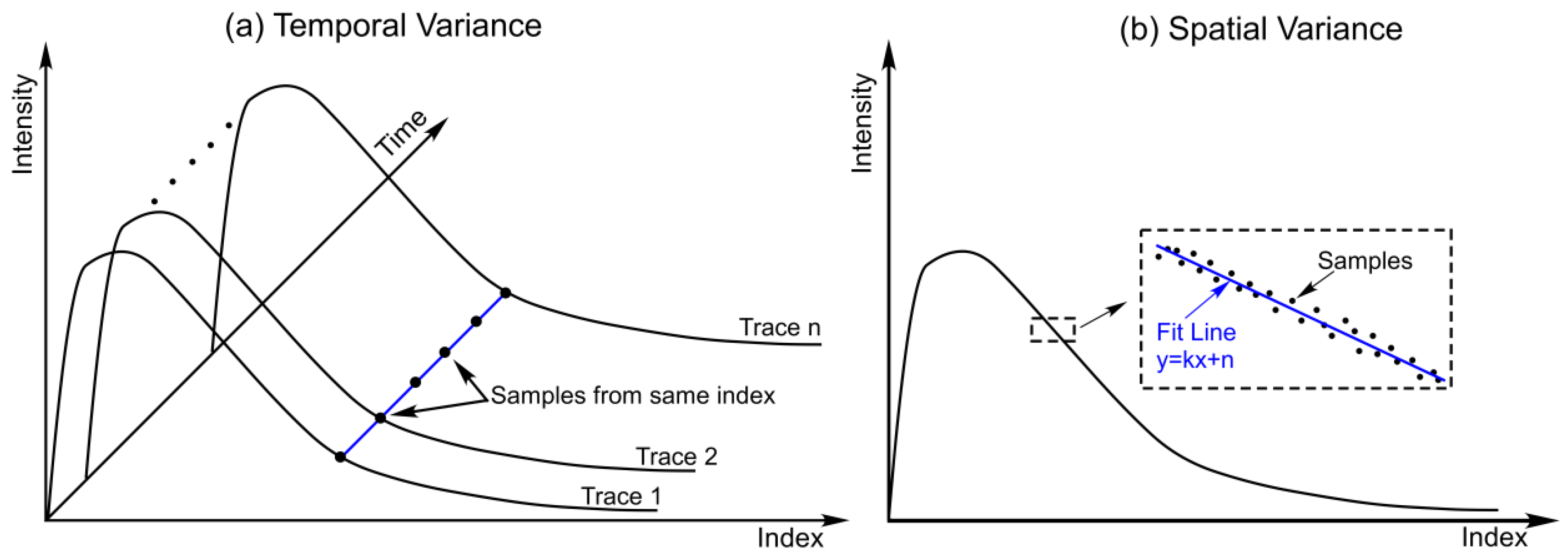It can be seen that the lidar returns are inversely proportional to the range squared r². Moreover, the temporal integrations of lidar measurements are performed to construct one probing profile in the data acquisition procedure to increase the signal to noise ratio. Therefore, the sample data distributions can be constructed in two ways for variance calculation: one is to select the data points from the fixed bin index (fixed range) in the successive probing traces, for expressing the atmospheric variation with time at a fixed height, which is called temporal variance; the other is to select consecutive data points from a fixed probing profile for expressing the atmospheric variation with a limited range interval at a fixed time, which is called spatial variance. The calculation models of temporal variance and spatial variance are shown in Figure 1.

In the calculation of temporal variance (Figure 1a), N_tv consecutive probing profiles with the same parameters of data acquisition are selected as the analysis objects. The sample data distribution is constructed using the data points at the same bin index (same range) from these probing profiles, the variance of which is to measure the spread of atmospheric information with time variation. In the calculation of temporal variance, the unbiased estimate of the variance σ² is expressed as:

$${\sigma }^2=\frac{1}{N_{tv}-1}{\displaystyle \sum _{i=1}^{N_{tv}}{\left(y_i-\mu \right)}^2}$$

(2)

where μ is the mean of the sample data distribution, and y is the data from the sample data distribution. For one lidar measurement, the number of sample data distributions for temporal variance calculation should be the number of data points N of the whole probing profile.

In the calculation of spatial variance (Figure 1b), only one probing profile is selected as the analysis objects. The sample data distribution is constructed using the data points from the N_sv consecutive bin indices along the probing trace, the variance of which measures the spread of atmospheric information with space variation. A linear fit parameterized with the slope k and the intercept n is done in each sample data distribution, as the lidar return signals are normally decreasing along the probing trace. As two additional parameters are introduced in the calculation of spatial variance, the unbiased estimate of the variance σ² should be modified as:

$${\sigma }^2=\frac{1}{N_{sv}-2}{\displaystyle \sum _{i=1}^{N_{sv}}{\left[y_i-\left(k{x}_i+n\right)\right]}^2}$$

(3)

where y is the data in the sample data distribution, and x could be the bin index in the sample distribution or the bin index along the trace. For one probing profile, the number of sample data distributions for spatial variance calculation should be (N − N_sv + 1), where N is the number of data points of the whole probing trace.

3. Data Distribution Characteristics of the Lidar Probing Traces

In principle, the variance calculation models for evaluating the data distribution characteristics of lidar probing traces can be applied to any atmospheric lidar system. In this paper, the ultraviolet elastic scanning lidar was taken as the research object [23,24], and a probing profile with a summed result of 20 laser shots or the lidar scanning profiles with a fixed elevation angle was analyzed to calculate the spatial and temporal variance. Based on the variance calculation results, the techniques for evaluating and improving the lidar performance were studied and implemented.

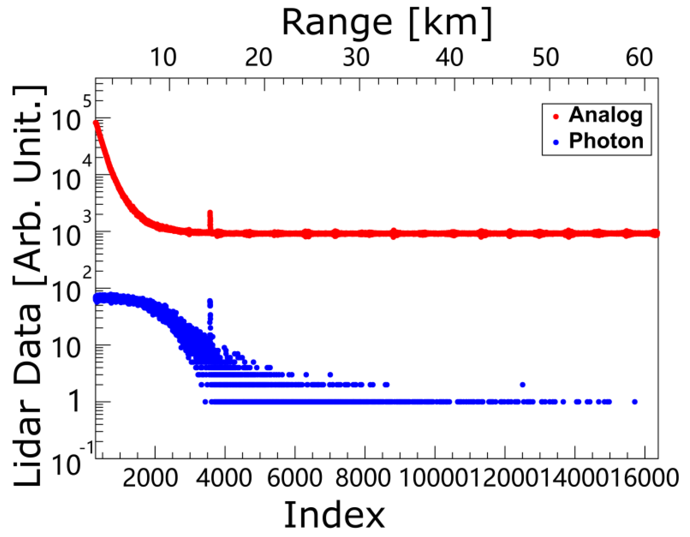
In ultraviolet elastic scanning lidar, the PMT of Hamamatsu R9880 (Hamamatsu Photonics K. K., Hamamatsu, Japan) was selected as the photo-electric converter, and the Licel transient recorder TR40-160 (Licel GmbH, Berlin, Germany) was chosen as the data acquisition system, as it can provide the analog detection mode and PC detection mode simultaneously. It has a range resolution of 3.75 m and a maximum detection range of 61.4 km. Figure 2 shows the raw probing traces of analog data and PC data from the ultraviolet elastic scanning lidar, which is a summed result of 20 laser shots. The raw data in PC mode is expressed using photons, while the raw data in analog mode is expressed by the values from the A/D acquisition card (for a 12 bit A/D, the maximum value is 4095, corresponding to 500 mV). Compared with the PC data, the analog data were more easily affected by the electronic noise of the data acquisition card.

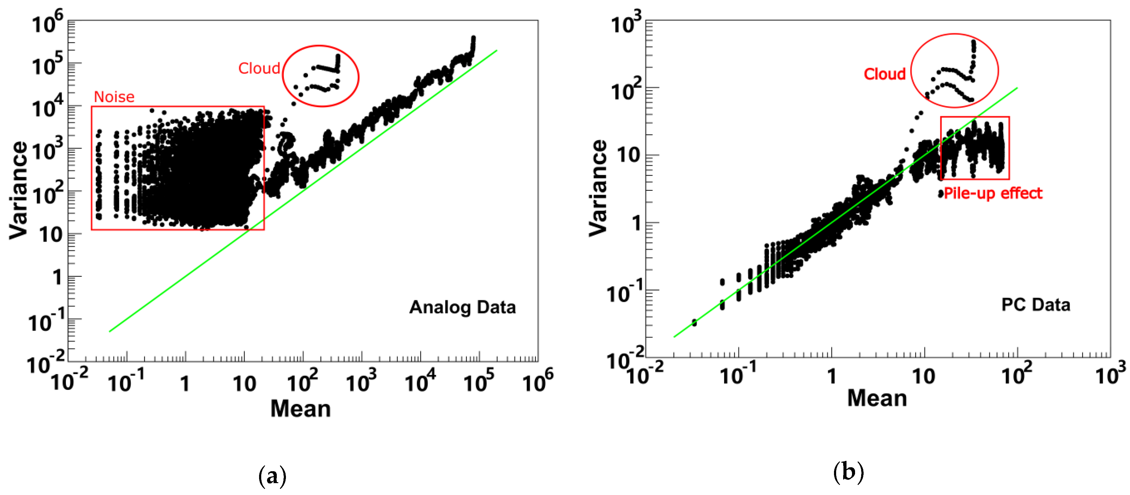
In the calculation of temporal variance, the successive probing profiles with a fixed elevation angle from the ultraviolet elastic lidar scanning measurements were selected as the study objects, as these probing profiles have the same lidar system constant. Figure 3 shows an example of the calculation results of temporal variance for both analog and PC data, which selected 14 successive probing profiles at the fixed elevation angle of 15° as the study objects and express the atmospheric variation within 14 s. It can be seen clearly that the data points of the noise signal in analog data are at the tail of the variance–mean scatter plot, and the data points of the PC data that suffered from the pile up effect are at the head of the variance–mean scatter plot. The data points of the cloud signals in both the analog and PC data are distributed in a disordered way in the variance–mean scatter plot. The variance values from the sample distributions of the normal lidar return signals in analog data are distributed parallel to the line of μ = σ², while the variance values from the sample distributions of the normal lidar return signals in PC data are distributed along the line of μ = σ². This shows that the PC data have the necessary condition of Poisson distribution, while the analog data do not have Poisson properties and have the potential to be converted to photon-like data using a linear transformation.

In the calculation of spatial variance, a single probing profile with a fixed elevation angle from the ultraviolet elastic lidar scanning measurements is selected was the study object. Figure 4 shows an example of the calculation results of spatial variance for both analog and PC data, which set N_sv to be 30 and expressed the atmospheric variation within a range interval of 112.5 m. The scatter plots of the spatial variance distributions from the analog data and PC data are similar, with the scatter plots of the temporal variance distribution, including the noise components in the analog data, the pile-up effect in PC data, and the cloud signals in both analog data and PC data. Compared with variance values from the sample distributions of the normal lidar return in the PC data along the line of μ = σ², the spatial variance values from the sample distributions of the normal lidar return signal in the analog data are parallel to the line of μ = σ², showing the potential of analog data to be converted to photon-like data using a linear transformation.

If we count the number of sample distributions displayed in the scatter plots of the temporal variance and spatial variance, it is found that not all of the sample distributions are confined within the theoretical number of the sample distributions in the temporal variance and spatial variance calculations (Figure 5). As the analog data are the summed results of the lidar returns and the electrical noises are from A/D cards, the effective number of sample distributions displayed in the scatter plots is coincident with the theoretical number. However, the effective number of sample distributions for both the temporal variance and spatial variance of PC data is less than the theoretical number, because in the far field, the PC system cannot detect extremely weak signals and return a PC data record with zero value. The effective number of the lidar data is measured using variance calculation results, with the consideration of avoiding the random effect of zero value. Based on this phenomenon displayed on the scatter plots of spatial variance and temporal variance, especially for the PC data, optimization of data acquisition parameters and calibration of lidar data were performed, including evaluation of the linear working range of the photo-electronic device, the estimations of the optimal discriminator level and dead time of PC system, and a novel technique of data gluing between analog data and PC data, which are described in detail in the following sections.

4. Optimization of Data Acquisition Parameters and Calibration of Lidar Data

A Licel transient recorder provides two detection modes simultaneously for PMT application: one is the analog detection mode, which uses the A/D card; the other is the PC detection mode, which uses the PC system. The high voltages applied in PMTs must be set in the linear working range to get the optimal gain for enhancing the performance of the lidar system, and the working range is influenced by weather conditions or specifications of lidar system. The evaluation of the linear working range of PMT is meaningful in the calibration of lidar data.

Moreover, the PC detection system comprises a discriminator and a counter. The discriminator is used to discriminate the voltage level of the pulse height of the PMT output, while the counter is to count the number of effective light pulse signals. Therefore, the preset threshold voltage of the discriminator is important in data acquisition procedures, as the final results of PC data is determined by this preset threshold voltage. Meanwhile, with the increase of the light intensity, the response of the PC system becomes nonlinear, because the output count rate is no longer proportional to the incident light intensity [25]. The estimation of the dead time plays an important role in the correction of pile-up effects in PC data.

Finally, a novel technique based on variance calculation for data gluing between analog data and PC data is presented in order to produce a uniform expression of a lidar trace.

4.1. Estimation of Dead Time of Photon-Counting System for Corrections of Pile-Up Effects

Due to the existence of dead time in a PC detection system, the observed count rate will be increased or decreased compared with the true count rate, resulting in pile-up effects of the electronic pulse in the data acquisition system. In a Licel transient recorder, the PC system is the non-paralyzable system [26], with a maximum count rate of 250 MHz and sample time of 25 ns. The relationship between the true photons N′ and observed photons N from a single photon pulse is:

$$N^{\prime }=\frac{N}{1-N\frac{{\tau }_d}{{\tau }_s}}$$

(4)

where τ_s is the sampling time and τ_d the dead time. When the lidar data is a summed result of laser echo signals excited by m laser pulses, the true photons n′ and the observed photons n have the following relationship:

$$n^{\prime }=\frac{n}{1-\frac{n}{m}\frac{{\tau }_d}{{\tau }_s}}$$

(5)

From the scatter plots of spatial variance and temporal variance of PC data, it can be seen that the variance values from the sample distributions of the PC data that suffered from the pile-up effect are out of the line of μ = σ². However, when the PC data is calibrated using Equation (5), the variance distribution is changed as well, which shows that the dead time of the PC system can be investigated by minimizing the differences between the variance and the mean as:

$${\chi }^2={{\displaystyle \sum _i[{\sigma }^2(P_i)-\mu (P_i)]}}^2$$

(6)

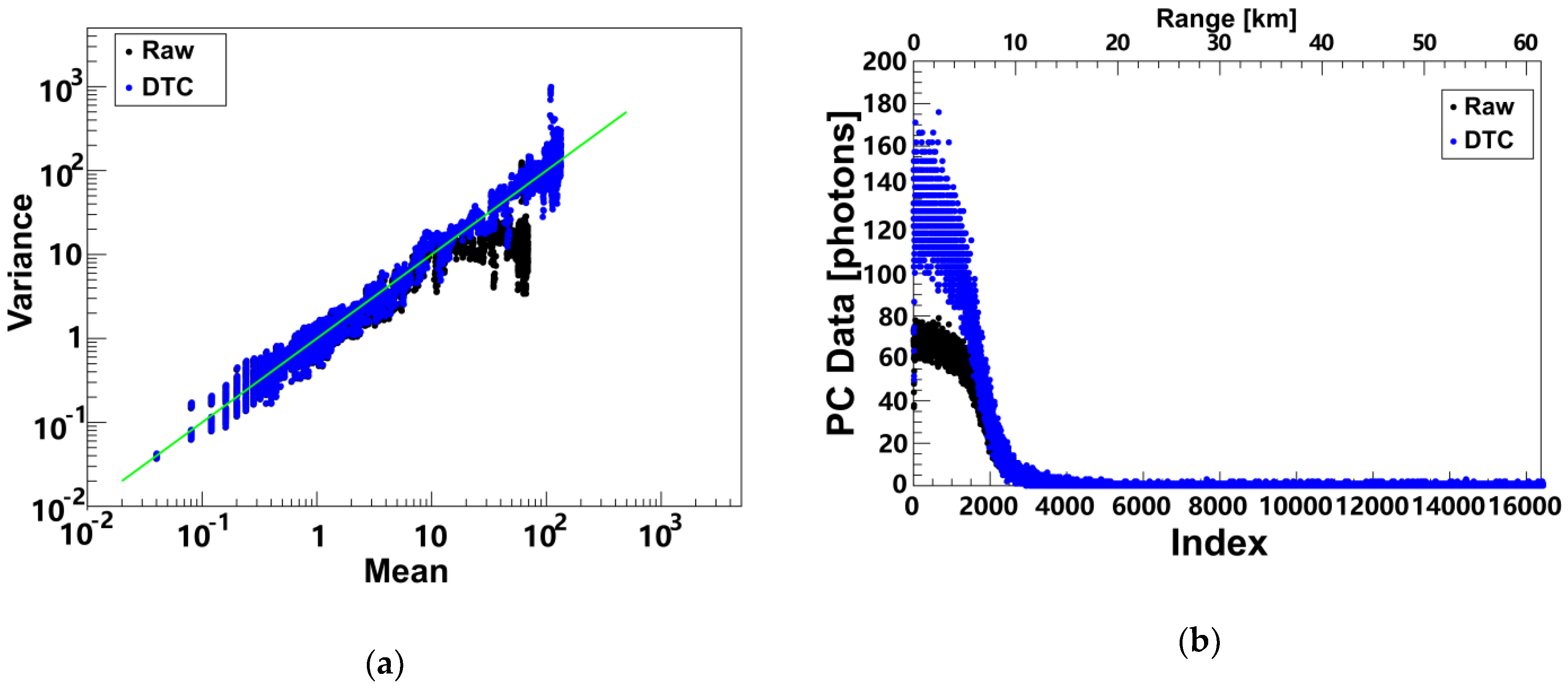
The calibrated PC data trace will have the maximum data distributions to be contributed Poissonian, which has the characteristics of the equality between the variance and the mean. The dead time of the PC system of the Licel TR40-160 transient recorder was estimated to be 3.488 ns by processing the 48 probing profiles from the scanning measurements of the ultraviolet elastic scanning lidar [27]. Figure 6 shows the estimations of the dead time of the PC system for the correction of pile-up effects. It can be seen that after the dead time correction (DTC), the PC data are mostly distributed according to a Poisson distribution, and more PC data points in near range can be used to express the atmospheric information.

4.2. Estimations of the Optimal Threshold Voltage of Photon-Counting System

In a PC system, when the voltages of the pulse heights of the PMT outputs are higher than the threshold voltage, the discriminator will produce a series of electronic pulses with a standard shape and height and send them to the counter. Therefore, the setting principle of the threshold voltage of a PC system is to record the actual lidar return signals and suppress the noise signal maximally, which can be analyzed based on the distributions of the pulse heights of the PMT outputs.

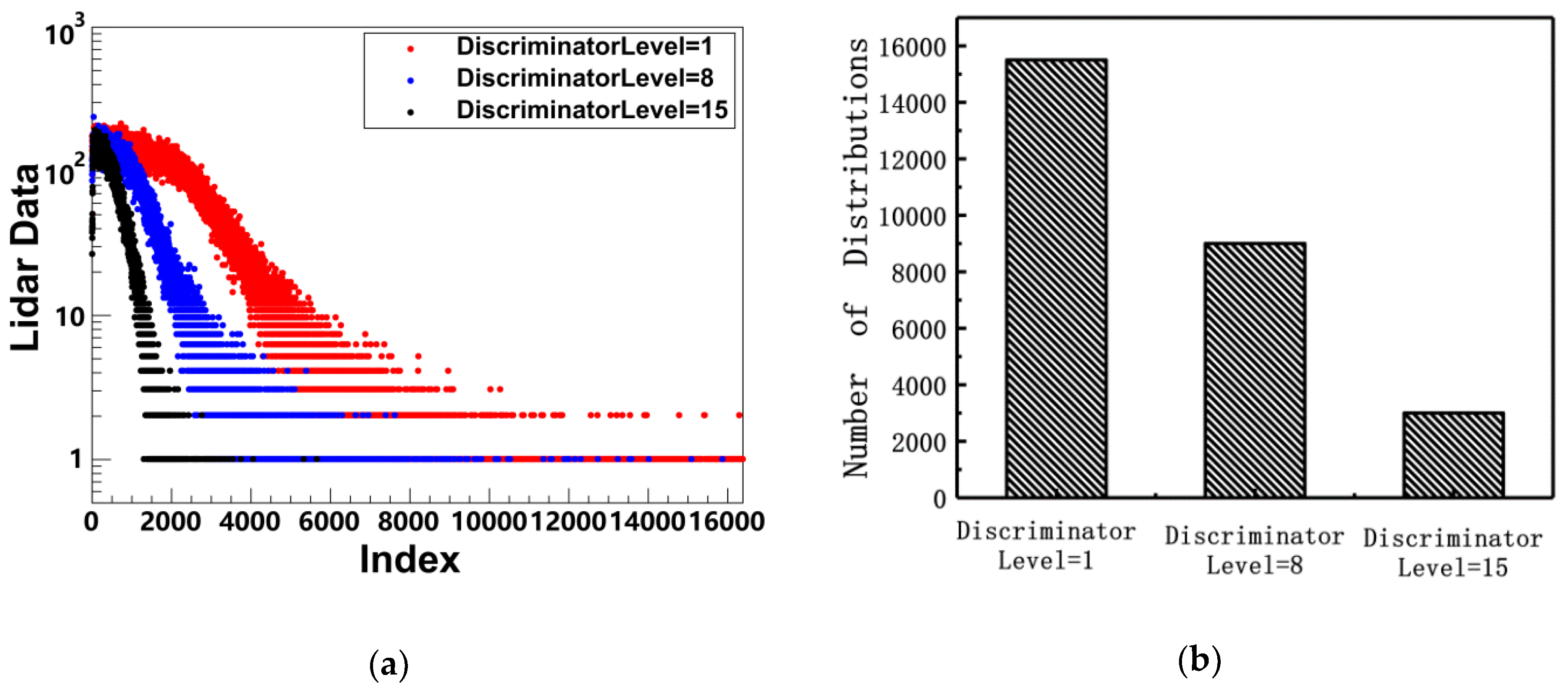
For the Licel transient recorder TR40-160, the threshold voltage can be preset between 0 mV and 25 mV using 64 discriminator levels, which means the step voltage is 0.40 mV. Figure 7a shows examples of the lidar profile of the PC data with different settings of threshold voltage at the same atmospheric conditions. The discriminator levels of 1, 8, and 15 correspond to the threshold voltages of 0.40 mV, 3.20 mV, and 6.00 mV, respectively. Not only is the lidar detection range related to the setting of the discriminator levels (Figure 7a), but the number statistics of non-zero data distributions are also related to the settings of the threshold voltage (Figure 7b).

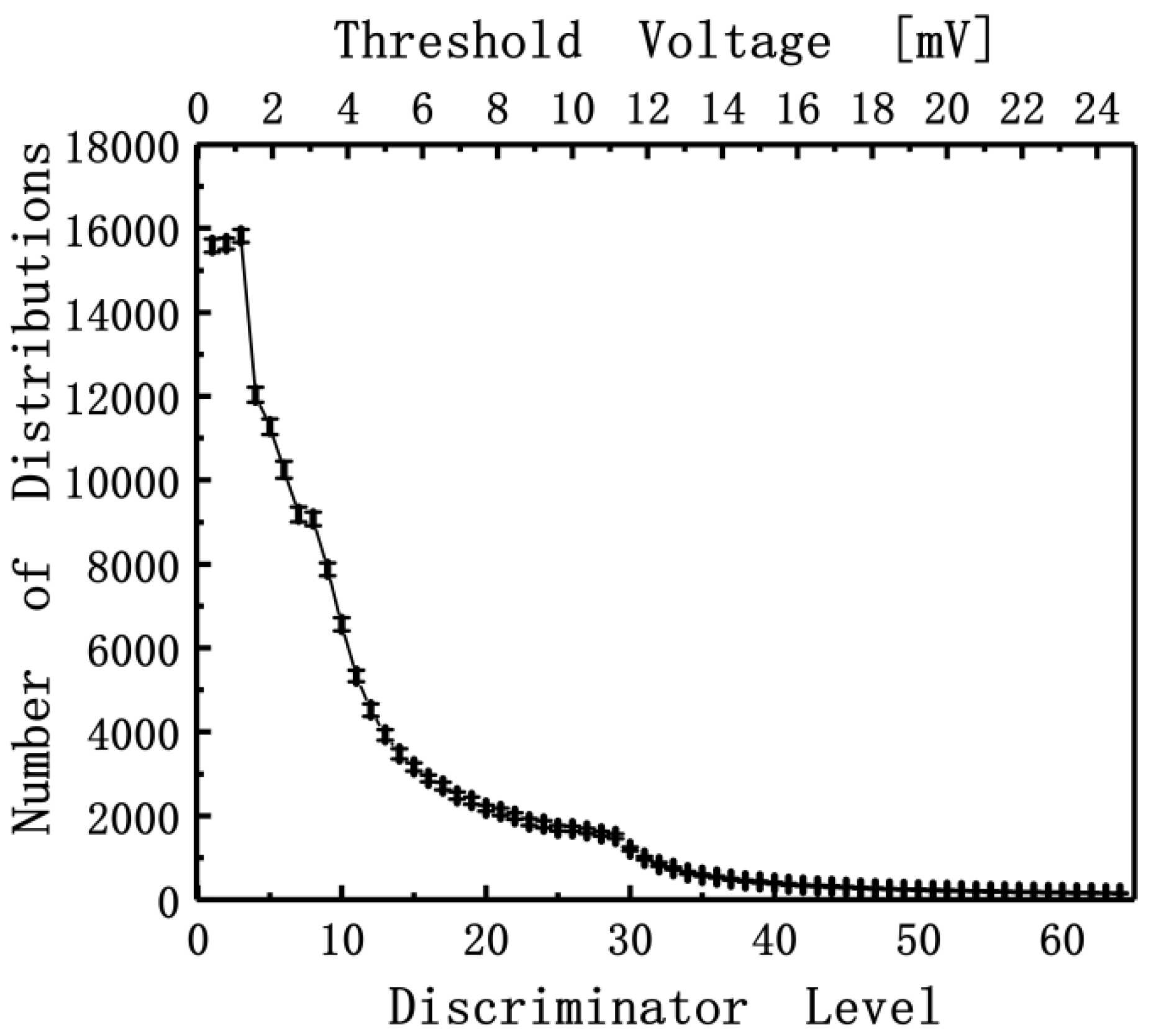
Figure 8 shows the number statistics of non-zero data distributions in the clear atmospheric conditions. It can be seen that the number of non-zero PC data points had its maximum value at the discriminator level of 3 (corresponding to the threshold voltage of 1.20 mV). When the preset threshold voltage was less than the threshold voltage of discriminator level 3, the PC system was susceptible to RF noise, combined with the pulse pile-up effect in near range, resulting in fewer non-zero points compared with that of discriminator level 3. When the preset threshold voltage was greater than the threshold voltage of discriminator level 3, the PC system was not powerful enough to discriminate the lidar echo signal from the far field. The number of non-zero data points in the probing profile decreased with the increased preset of the threshold voltage. Based on such analysis, it was concluded that the optimal discriminator level of Licel transient recorder TR40-160 in the ultraviolet elastic scanning lidar is 3, corresponding to the threshold voltage of 1.20 mV, which makes the maximum lidar detection range of the ultraviolet elastic scanning lidar.

4.3. Evaluation of the Linear Working Range of the PMT

With a power supply providing high voltage up to kilovolts, the PMT can work and convert the light pulse to the electrical signal. Meanwhile, the high voltage must be set in a linear working range, which results in a gain in the linear transform region. However, in lidar applications, the intensities of the lidar returns are inversely proportional to the range squared, which may result in a strong detection capability in far range but a saturation signal in near range. In Raman lidar or high-spectral-resolution lidar with multi-channels, the intensities of the separated spectral radiant flux in different channels are different, and the PMT may be set with different high voltages to achieve the optimal detection performance. Therefore, to make the received lidar returns normalized in the procedure of data retrieval, the evaluation of the linear working range of the PMT is necessary in the construction of the lidar system.

In order to explore the linear working range of the PMT, a programmable high voltage system of PMT is designed to realize fast data acquisition of real-time laser echo signals with different high voltages under the clear atmospheric conditions. Figure 9 shows the spatial variance distribution of the PC data with different high voltages of PMT settings in clear atmospheric conditions. It can be seen that the detection capability of the ultraviolet elastic scanning lidar changes significantly with the settings of the PMT high voltages. Although the phenomenon of the pile-up effect in PC data is lessened with the decrease of the high voltages, the maximum value of PC data with a high voltage of 900 V was more than ten times of the PC data value with a high voltage of 600 V.

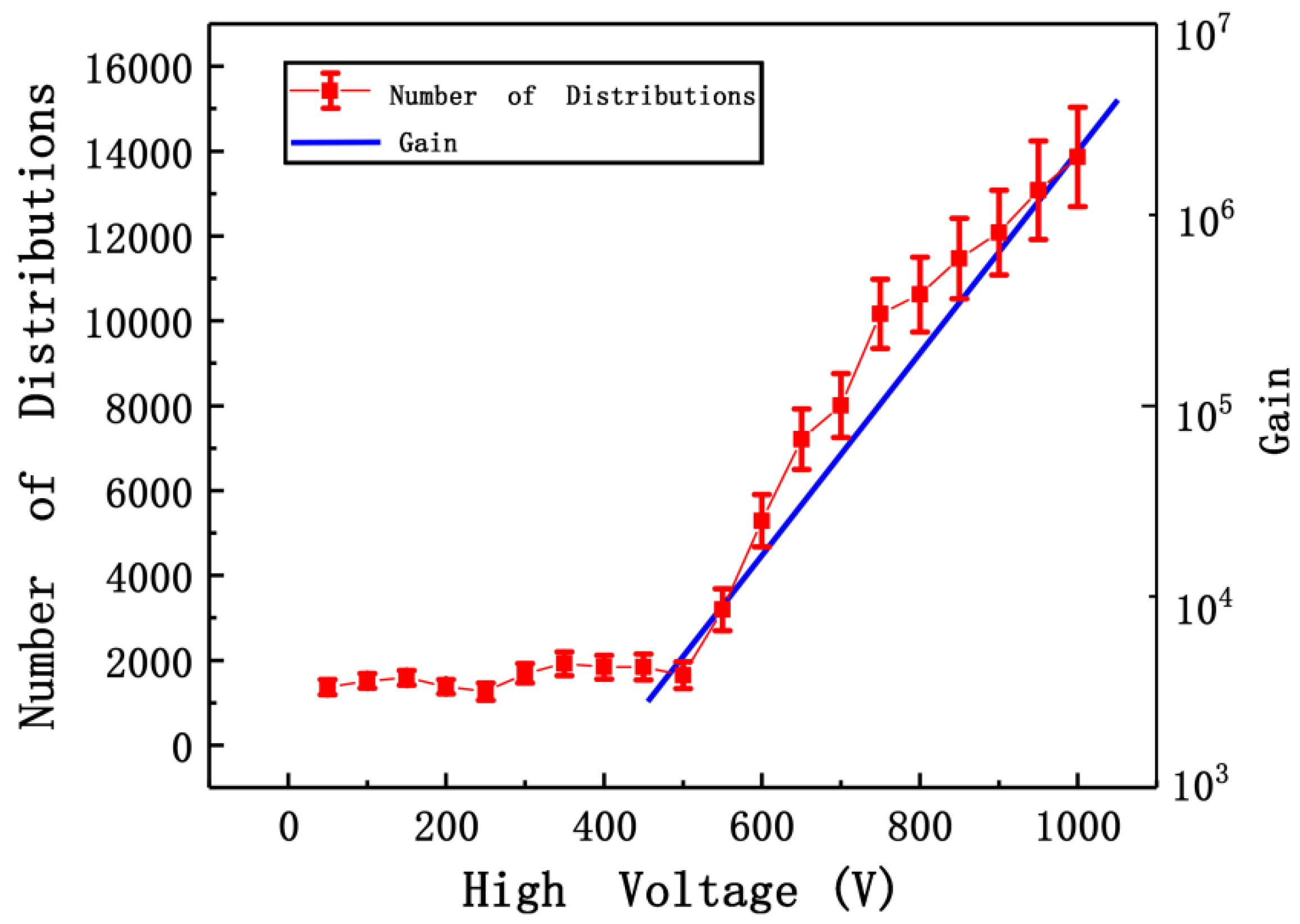
Figure 10 shows the statistics results of the non-zero PC data with different high voltages of the PMT settings under clear atmospheric conditions. It can be seen that when the absolute values of high voltage were less than 500 V, the number of non-zero PC data were less than 3000 and remained constant. However, when the absolute values of high voltage were larger than 500 V, the number of non-zero PC data linearly increased with the high voltage settings, which indicates that the linear working range of the PMT is between −500 V and −1000 V and corresponds to the gain curve of the PMT.

4.4. Data Gluing between Analog Data and Photon-Counting Data

Whatever the calculation results of temporal variance and spatial variance, the analog data is not distributed according to a Poisson distribution, as its variance distribution is not equal to the corresponding mean values. However, the scatter plot of the variance–mean distribution is parallel to the straight line y = x, indicating that the analog data can be transformed to the PC-like data by a linear transformation, and the transformed PC-like data will have the characteristic of equality between the variance values and the mean values. If both analog data and PC data have an identical variance–mean distribution, the data traces could be uniformly merged by definition without any further requirement. The merging could thus be achieved by modifying analog data (A) into the transformed PC data (A′), using a linear transformation:

$$A^{\prime }=aA+b$$

(7)

and the transfer coefficients a and b can be determined by minimizing the distance between the mean and the variance for all transformed PC data points (A′) as:

$${\chi }^2={{\displaystyle \sum _i[{\sigma }^2(A_i^{\prime })-\mu (A_i^{\prime })]}}^2$$

(8)

In the retrieval of the transfer coefficients, only the analog data with a high signal to noise ratio (>10) can contribute to the retrieval procedure. Figure 11 shows the retrieval results of the transfer coefficients a and b, which are 0.2431 and −225.0, respectively. The variance–mean scatter plots of the raw analog data (SNR > 10 in near field) and the transformed PC data show that most of the transformed PC data have the necessary condition of Poisson distribution, in which the variance and its corresponding mean are basically equal.

By linear transformation using the transfer coefficients a and b, the analog data are shifted to the transformed PC data. Figure 12a shows the matching conditions between the transformed PC data and the PC data after dead time correction. It can be seen that within the bin index of 2000–3000, these two data traces are basically coincident. The merging point is selected at the position with the smallest dispersion between these two data traces, which makes the normalized lidar data trace constructed with the transformed PC data in the near field and the PC data after dead time correction in the far field (Figure 12b). The normalized lidar data trace improves the lidar detection capability and expresses the atmospheric condition uniformly.

5. Discussion

In this paper, most of the works were implemented using spatial variance, considering that the lidar system constant remains unchanged in a single probing trace. Within a limited range interval, the distributions of the spatial variance were more stable than the distributions of the temporal variance, in which multiple lidar probing traces were used to construct the sample distributions. The results of the temporal variances not only show the variation of atmospheric condition with time, but also present the variations of the lidar system constant in different probing profiles, especially the influences of the laser jitter. The concept of temporal variance was proposed for studies of the time scale of the atmosphere. Although the technique of data merging is performed using the spatial variance calculation, the calculation of temporal variance can be applied using data merging as well, which produces a similar result as the spatial variance.

The traditional method for data merging between analog data and PC data is to investigate the transfer coefficients a and b by minimizing the differences between the transformed PC data and the raw PC data within a linear region with the count rate range of 1–20 MHz [15,28]. The lower count rate and upper count rate of the linear region are affected by atmospheric conditions and by the performance of the data acquisition hardware, as the A/D card for analog detection mode and the PC system for PC detection mode are two independent devices [15]. Recorded data can be affected by ground noise in the analog detection chain and by discriminator level in the PC detection chain, which makes the linear region system-dependent and results in relatively large transformation errors due to different linear intervals [29]. The distributions of the transfer coefficients a and b for a number of data traces obtained from the scan measurements were investigated using both the variance-based gluing method and the traditional method, which are shown in Figure 13. For both merging methods, an identical linear relationship between a and b was found, with about 5% difference in the slope. The longitudinal distribution of trace characteristics (points with coordinates defined by a and b values) along the fitted line was found to be Gaussian in the case of variance-based gluing. In the case of the traditional method, no smooth functional dependence cloud be found, which implies that this method was more affected by the variation of the atmospheric condition in the lidar field of view. This paper provides a new idea for data merging between analog data and PC data, which makes the glued profiles have the uniform properties of variance–mean distributions.

In both investigations of the dead time of the PC system and the transfer coefficients a and b in variance-based data gluing (Equations (6) and (7)), the results were weighted by the larger values due to the large dynamic range. In the estimation of the dead time of the PC system, the research purpose was to correct the pile-up effect of PC data, which influenced the accuracy heavily when using the head part of the PC data with larger values. However, in the data gluing, only the analog data with a range interval starting at the head of the trace to where the signal to noise ratio was continuously greater than 10 were contributed to the retrieval procedure. The transfer coefficients a and b were used to transform the analog data to PC-like data using a linear transformation, especially the head of the analog data, which is the head part of the normalized lidar data trace used to uniformly express atmospheric conditions.

6. Conclusions

The equivalence between the variance and the mean is the characteristic of the Poisson distribution of this data set. In this paper, calculation models for temporal variance and spatial variance were constructed to evaluate the variance–mean distribution characteristics of lidar analog data and PC data. The calculation results show that both the spatial variance and the temporal variance of the PC data distributions in far field were basically equal to their mean, while the PC data in the near field do not conform to the Poisson distribution due to the pile up effect. The variances of the analog data were not equal to their mean, meaning that the analog data do not conform to the Poisson distribution, but the data in near field had the potential to be converted to PC-like data using linear transformation.

To make the spatial variance equal to their corresponding mean in the variance–mean plots, the dead time of the Licel TR40-160 in ultraviolet elastic scanning lidar was estimated to be 3.488 ns. The optimal threshold voltage of the PC system and the linear working range of the PMT were evaluated using the number of non-zero PC data, which was counted using the variance distribution. The experimental results show that the optimal threshold voltage of the PC system in Licel TR40-160 is 1.20 mV, and the linear working range of the high voltages of the PMT is between −500 V and −1000 V.

A novel method for data gluing between analog data and PC data is proposed based on variance calculation. The analog data can be transformed to PC-like data by a linear transformation, in which the transfer coefficients are investigated by minimizing the differences between the variances and their corresponding means. The experimental results show that the normalized lidar data trace improved the lidar detection capability and expressed the atmospheric condition uniformly.