A Comparative Study of Various Methods for Handling Missing Data in UNSODA

Abstract

UNSODA, a free international soil database, is very popular and has been used in many fields. However, missing soil property data have limited the utility of this dataset, especially for data-driven models. Here, three machine learning-based methods, i.e., random forest (RF) regression, support vector (SVR) regression, and artificial neural network (ANN) regression, and two statistics-based methods, i.e., mean and multiple imputation (MI), were used to impute the missing soil property data, including pH, saturated hydraulic conductivity (SHC), organic matter content (OMC), porosity (PO), and particle density (PD). The missing upper depths (DU) and lower depths (DL) for the sampling locations were also imputed. Before imputing the missing values in UNSODA, a missing value simulation was performed and evaluated quantitatively. Next, nonparametric tests and multiple linear regression were performed to qualitatively evaluate the reliability of these five imputation methods. Results showed that RMSEs and MAEs of all features fluctuated within acceptable ranges. RF imputation and MI presented the lowest RMSEs and MAEs; both methods are good at explaining the variability of data. The standard error, coefficient of variance, and standard deviation decreased significantly after imputation, and there were no significant differences before and after imputation. Together, DU, pH, SHC, OMC, PO, and PD explained 91.0%, 63.9%, 88.5%, 59.4%, and 90.2% of the variation in BD using RF, SVR, ANN, mean, and MI, respectively; and this value was 99.8% when missing values were discarded. This study suggests that the RF and MI methods may be better for imputing the missing data in UNSODA.

1. Introduction

Soil properties, including bulk density (BD), water content (WC), particle density (PD), porosity (PO), saturated hydraulic conductivity (SHC), organic matter content (OMC), and pH, can be divided into physical properties and chemical properties [1]. OMC and pH are the most important chemical properties. They have significant effects on plant growth [2,3,4]. Physical properties, such as SHC, BD, WC, PD, and PO are frequently measured to calculate soil’s hydraulic properties [5,6,7,8,9] or to characterize soil compaction [10,11]. BD is also widely used as an essential parameter for soil weight-to-volume conversion, especially when calculating the carbon and nutrient contents of a soil layer [12]. SHC is also used to calculate water flux in a soil profile and to design irrigation and drainage systems [13].

In theory, data on these soil properties can be obtained directly through experiments, but in practice, direct measurements are difficult and labor-intensive, and the data are highly variable, particularly for properties such as BD [12,14,15,16,17]. In addition, the measurement of soil–water characteristic curves and unsaturated soil hydraulic conductivity is also time-consuming and labor-intensive [9,18]. For these reasons, methods have been developed to use property data with low variability to estimate soil properties which are difficult to measure directly; these estimation methods are called pedotransfer functions (PFTs) [19,20], and they are commonly data-driven. One of the advantages of these data-driven models is that they are usually far more flexible than standard statistical models and can capture higher-order interactions between the data, resulting in better predictions. For this reason, the role of soil property data is becoming more and more important, and a number of soil property datasets have been established. Among them, the Unsaturated Soil Database (UNSODA) [21,22], the European Database of Soil Hydraulic Properties (HYPRES) [23], SoilVision, and the Harmonized World Soil Database (HWSD) [24] are the most representative. The UNSODA database has been widely used because it provides a large amount of information free of charge. For example, Huang and Zhang [25], Hwang and Powers [26], Hwang et al. [27], Mohammadi and Vanclooster [28], and Chang and Cheng [29] predicted SWCCs using particle size distribution data; Ghanbarian-Alavijeh et al. [30] used soil texture data; and Haverkamp et al. [31], Seki [32], Ghanbarian and Hunt [33], Pham et al. [34], and Vaz et al. [35] used soil properties such as BD, PO, and others.

However, there are missing soil property data in UNSODA for pH [pH] (pH), saturated hydraulic conductivity [k_sat] (SHC), organic matter content [OM_content] (OMC), porosity [porosity] (PO), particle density [particle_density] (PD), and bulk density [bulk_ density] (BD). The square brackets represent the features in the original tables and round brackets represent the features used in this study.

Missing data, a real-world problem often encountered in scientific settings, is problematic because many statistical analyses require complete data. Researchers who want to perform a statistical analysis that requires complete data are forced to choose between imputating data and discarding missing values; the latter is the most common method of using the UNSODA. However, discarding missing data may not be reasonable when the proportion of missing data is not small, as valuable information may be lost and inferential power compromised [36]. According to Strike et al. [37] and Raymond and Roberts [38], when the dataset contains a very small amount of missing data, e.g., the missing rate is less than 10% or 15% across the whole dataset, missing data can simply be removed without loss of valuable information. However, when the missing rate exceeds 15%, the missing information may reduce insights into the data [39], especially when dealing with the extraction of knowledge from a given dataset; therefore, careful consideration should be given to handling of missing data. Missing values are of different types, and some of them are discussed below [40]:

(i)

Missing completely at random (MCAR): The missing data are not related to known values. With this type of missing data, we assume that a whole distribution of data is completely missing.

(ii)

Missing at random (MAR): The missing value depends on an already known value and does not depend upon the missing value itself.

(iii)

Not missing at random (NMAR): The missing value does not depend upon any given or missing value.

These different types of anomaly generally arise from different sources. Data MCAR may arise from sensor recording failure, and there may be no other data dependent on the missing data. By contrast, MAR may arise when some survey questions are not answered, yet there are other questions related to the unanswered items.

The data in UNSODA were mainly contributed by individual scientists, and some of the datasets were taken from the literature. A questionnaire based on suggestions from participants at an international workshop on soil hydraulic properties held in Riverside in 1989 was also used to request information for UNSODA [22,41].

The above discussion explains how UNSODA was created, but we still cannot confirm its type(s) of missing data. For imputation purposes, the missing values in UNSODA were supposed to be MAR.

The objective of this paper was to impute missing values in UNSODA; to our knowledge, this work has not been undertaken previously. The main missing features, such as pH, SHC, OMC, PO, and PD, were all included. After reviewing of existing missing value imputation techniques, we used the random forest (RF) regression method to impute the missing values in UNSOD. Its performance was then compared with the performances of both machine learning-based methods, i.e., support vector (SVR) regression and artificial neural network (ANN) regression, and statistics-based methods, i.e., mean and multiple imputation (MI) methods.

2. A Brief Review of Existing Missing Value Imputation Techniques

Imputation methods involve replacing one missing value with another value that has been estimated based on data mining of available information in the dataset [39]. Imputation methods can be divided into single and multiple imputation methods based on the number of values imputed [39,42]. According to the construction approach used for data imputation, these technologies can also be classified into statistics-based and machine learning-based (or model-based) methods [39]; the details of these approaches are listed in Table 1.

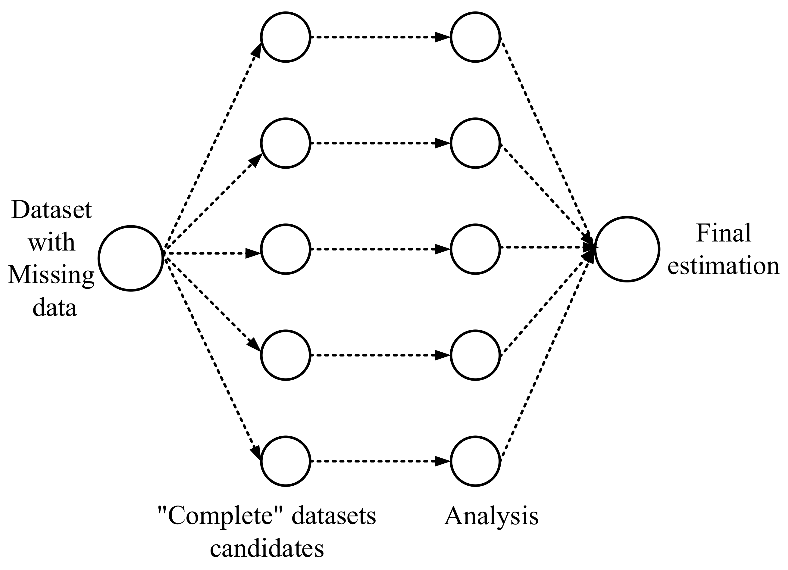
Statistics-based methods are a popular approach for missing data imputation in which a statistic (such as mean) is calculated for each column, and all missing values for that column are replaced with the statistic. The MI method is another widely used statistics-based method, which was first proposed by Rubin in the late 1970s [43]. Instead of imputing a single value for each missing data, multiple imputation creates many completed candidate datasets according to the missing data case, and then combines these candidate datasets into one estimate for the missing data. Machine learning techniques, such as the k nearest neighbor (KNN), RF, ANN, and SVR methods, have been widely employed in the last 20 years [44]. It should be noted that KNN approaches tend to perform poorly in high-dimensional and large-scale data settings.

Table 1. The main statistical-based and machine learning based imputation methods.

Statistics-Based	Machine Learning-Based
Expectation maximization (EM) [45]	Random forest (RF) * [36,46]
Hot deck (HD) [47,48]	Artificial neural networks (ANN) * [49]
Multiple imputation (MI) * [50]	Support vector regression (SVR) * [51]
Mean/mode * [52]	K-nearest neighbor (KNN) [53]
Gaussian mixture model (GMM) [54]	Decision tree (DT) [55]
	Clustering [55,56]

Note: * the imputation method used in this study.

Table 1. The main statistical-based and machine learning based imputation methods.

Statistics-Based	Machine Learning-Based
Expectation maximization (EM) [45]	Random forest (RF) * [36,46]
Hot deck (HD) [47,48]	Artificial neural networks (ANN) * [49]
Multiple imputation (MI) * [50]	Support vector regression (SVR) * [51]
Mean/mode * [52]	K-nearest neighbor (KNN) [53]
Gaussian mixture model (GMM) [54]	Decision tree (DT) [55]
	Clustering [55,56]

Note: * the imputation method used in this study.

3. The UNSODA Dataset and Procedure for Missing Value Imputation

3.1. The UNSODA Dataset

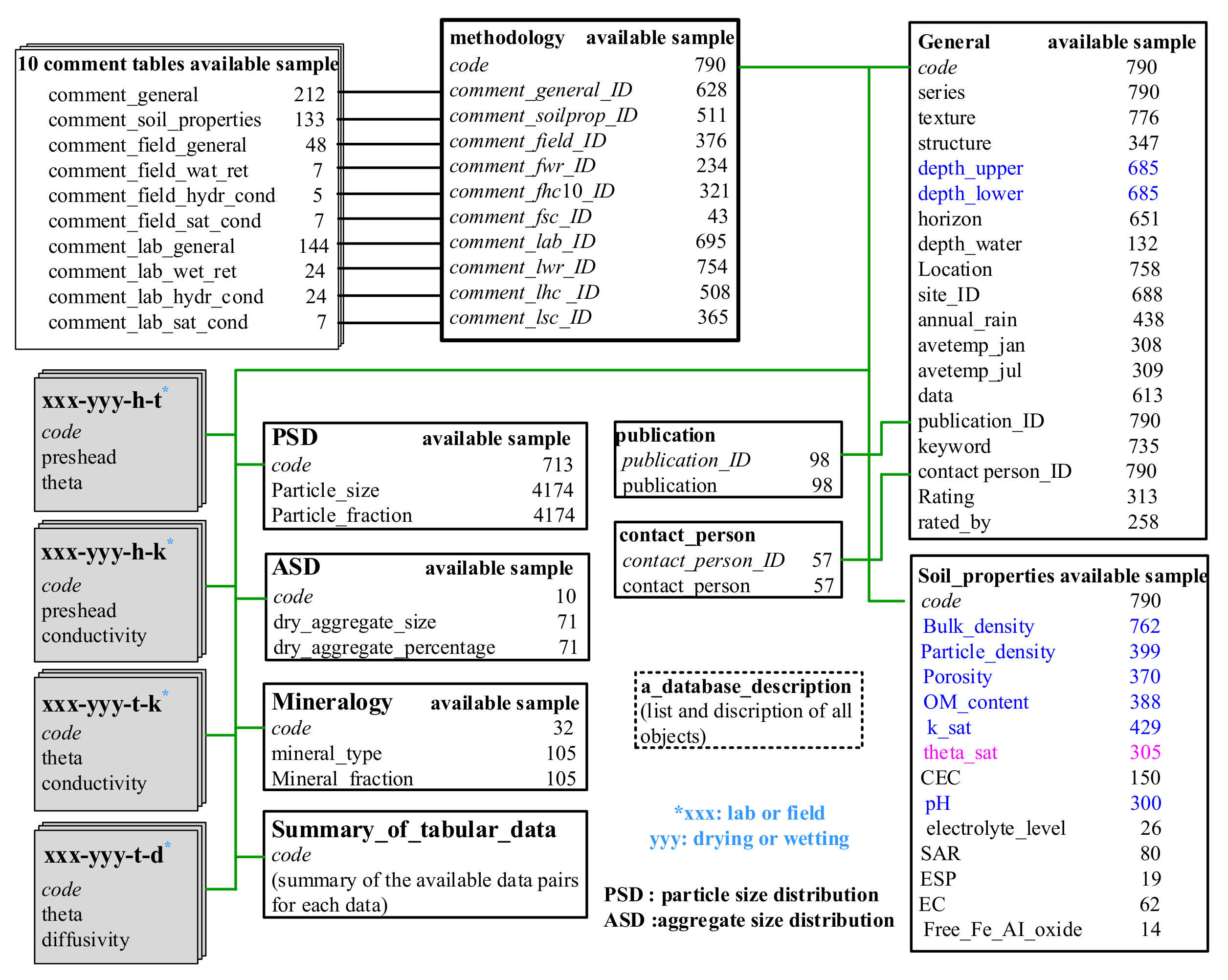
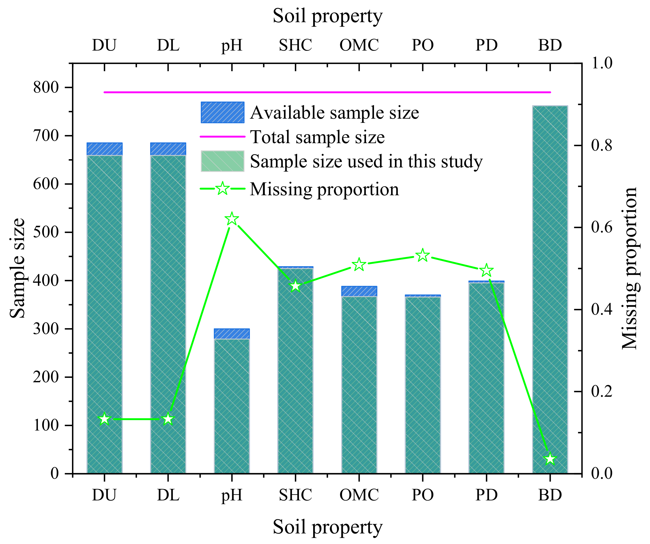
The structure of the database, names of tables, and links between tables are summarized in Figure 1. The main table of UNSODA is called “general”. It holds essential information about the soils, such as the geographic location, texture, classification, and environment of each. The “soil_properties” table contains physical and chemical properties for each soil, such as pH, SHC, OMC, PO, PD, and BD.

Table 2. Statistical descriptions of soil properties in UNSODA.

Soil Property	Effective Sample	Data Sample *	Range	Mean	Q1 (25%)	Q2 (50%)	Q3 (75%)	Missing Proportion **
DU	685	659	0∼325	41.231	5.000	30.000	61.000	0.1329
DL	685	659	0∼3000	72.466	30.000	56.000	95.000	0.1329
pH	300	279	3.1∼8.6	6.259	4.900	6.700	7.540	0.6203
SHC	429	425	0.019∼27,648	613.559	20.818	95.900	459.400	0.4570
OMC	388	367	0.01∼88.4	2.942	0.340	0.940	2.500	0.5089
PO	370	366	0.175∼0.915	0.469	0.405	0.456	0.510	0.5316
PD	399	395	1.65∼2.93	2.642	2.610	2.650	2.690	0.4949
BD	762	762	0.17∼2.1	1.444	1.340	1.490	1.600	0.0354

NOTE: * The data sample was deleted when BD was missing. ** Missing Proportion = missing sample/total sample (790).

summarizes the statistical descriptions for the distribution of soil properties. Figure 2 presents the available sample size, total sample size, and missing proportion of each soil property. Table 2 and Figure 2 show that there are a number of missing values for BD, PD, PO, SHC, OMC, and pH, and the missing proportions for these features are 0.0354, 0.4949, 0.5316, 0.4570, 0.5089, and 0.6203, respectively. To analyze the relationships between variables as comprehensively as possible, the upper depth [depth_upper] (DU) and lower depth [depth_lower] (DL) of the sampling locations are specified. The missing proportions of DU and DL are only 0.1329 and 0.1329, respectively. It should be noted that the sample size used in this study was smaller than available sample size. The main reason was that the available sample was deleted when the corresponding BD was missing.

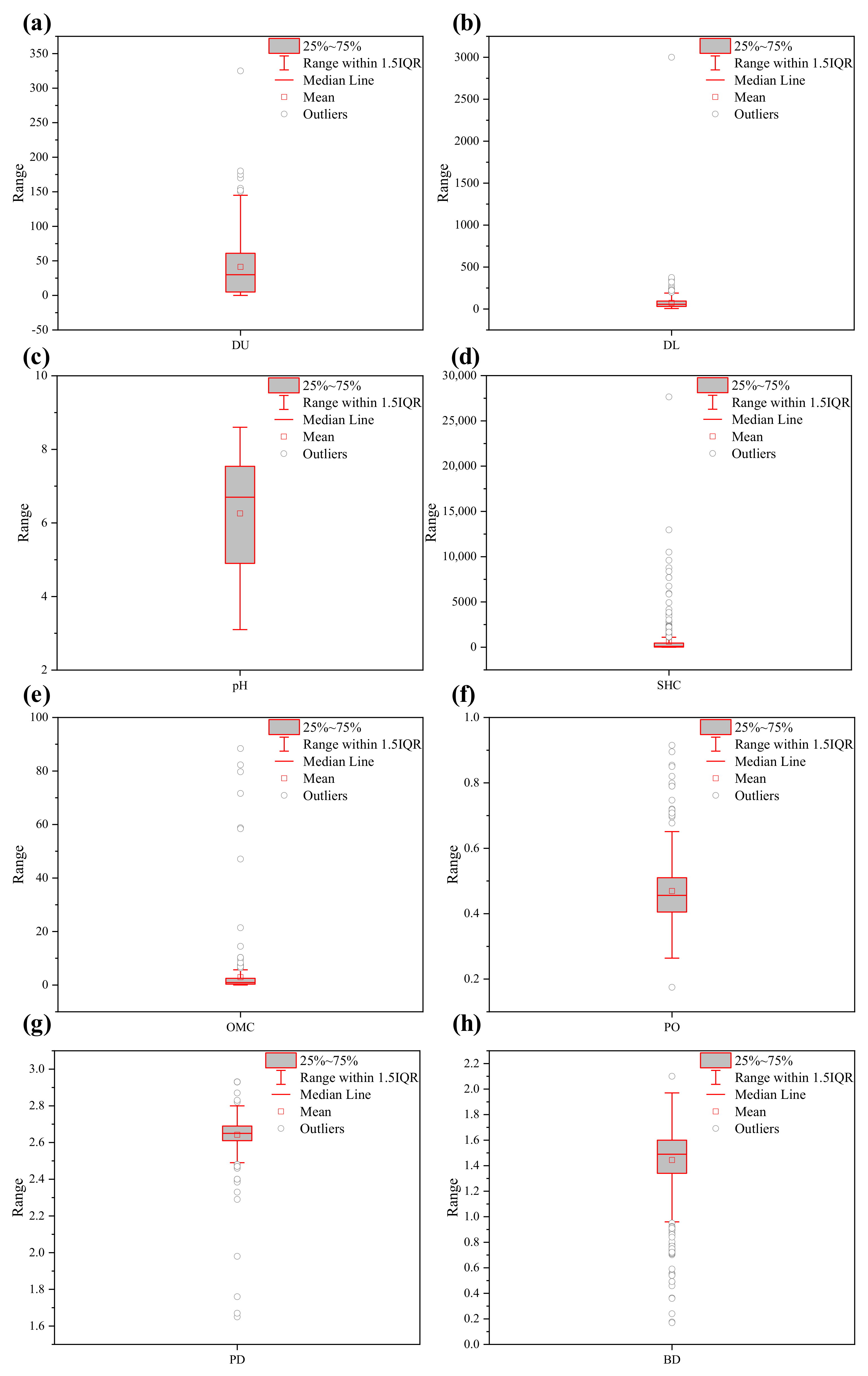
Figure 3 presents boxplots for the distributions of these soil properties. The statistical descriptions indicate that these features cover different scales. Among them, the SHC had the broadest range, i.e., 0.019–27,648, in which the distribution was mostly skewed toward low values in the range of 20.818 to 459.400. On the other hand, the distribution ratio of PO had the narrowest range, i.e., 0.175–0.915, which centered on the range of 0.405–0.510.

Furthermore, according to Tukey’s rule, 176 outliers, whose values were either higher than $Q3+1.5IQR$ or lower than $Q1-1.5IQR$ ($IQR=Q3-Q1$ is the interquartile range of the dataset; $Q3$ and $Q1$ are the first and third quartiles of the dataset, respectively) were detected in cases of DU, DL, pH, SHC, OMC, PO, PD, and BD, as shown in Figure 3. It should be noted that most of the outliers were observed in case of the SHC, i.e., 43 out of 176 outliers.

3.2. Procedure for Missing Values Imputation

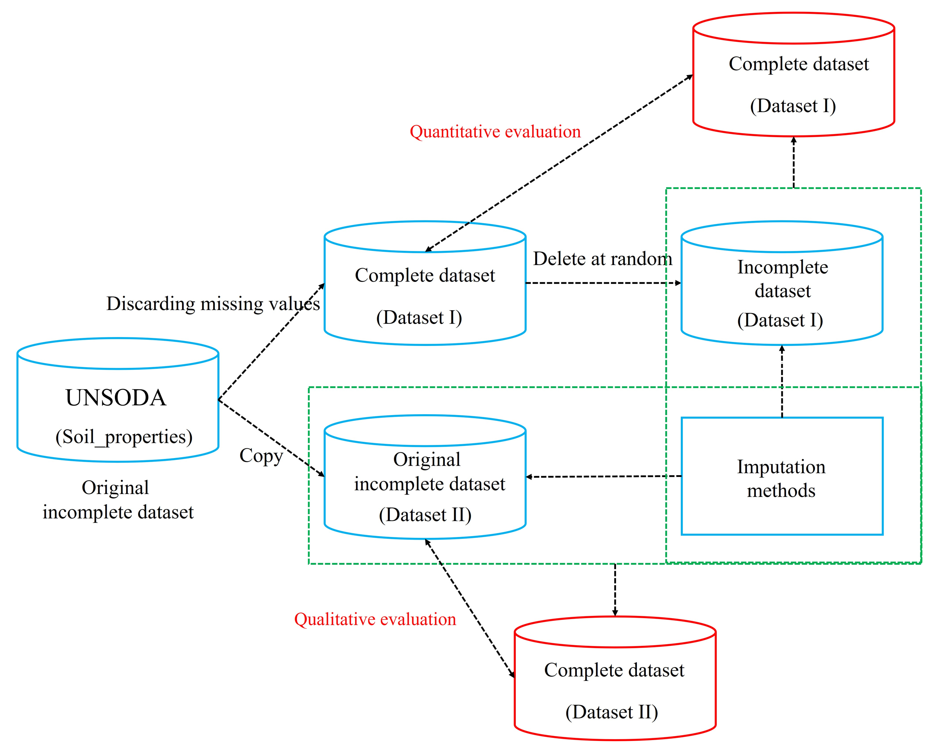
The experimental procedure for missing value imputation is shown in Figure 4. Before imputing the missing values in the original incomplete dataset, we first considered one complete dataset (Dataset I) (i.e., with missing values discarded). Once missing values were discarded, the number of datasets decreased significantly ($n=109$). Second, a missing value simulation was performed. That is, dataset I was simulated with different missing proportions (e.g., 3%, 7%, 11%, 15%, 19%, and 23%) using an MAR approach. Different incomplete datasets were produced with different proportions of missing data. The purpose of this design was to simulate and compare quantitatively the advantages and the drawbacks of the different imputation methods.

4. Methodology

In this Section, we introduce and describe the methods used to impute the dataset with the values deleted at random (Dataset I) and the original incomplete dataset (Dataset II).

(i)

Statistics-based methods, including mean and MI.

(ii)

Machine learning-based methods, including RF, SVR, and ANN.

4.1. General Notation

Let X be our $n\times p$ matrix of predictors that requires imputation [57]:

$$X=\left(X_1,X_2,X_3,\dots ,X_p\right)=\left(\begin{array}{ccc}{x}_{11}& \dots & x_{1p}\\ ⋮& \ddots & ⋮\\ x_{n1}& \cdots & a_{np}\end{array}\right)$$

(1)

An arbitrary variable $X_s$ contains missing values at entries $i_{mis}^{\left(s\right)}\subseteq \left\{1,2,\dots ,n\right\}$.

For every variable $X_s$ that contains missing values, we can separate the dataset into four categories:

(i)

Non-missing values of variable $X_s$, denoted by $y_{obs}^{\left(s\right)}$.

(ii)

Missing values of variable $X_s$, denoted by $y_{mis}^{\left(s\right)}$.

(iii)

Variables other than $X_s$, with observation $i_{obs}^{\left(s\right)}=\left\{1,2,...,n\right\}\setminus i_{mis}^{\left(s\right)}$, denoted by $x_{obs}^{\left(s\right)}$.

(iv)

Variables other than $X_s$, with observation $i_{mis}^{\left(s\right)}$, denoted by $x_{mis}^{\left(s\right)}$.

4.2. Statistics-Based Methods

4.2.1. Mean Imputation

Mean imputation is a simple imputation technique that calculates the mean of $y_{obs}^{\left(s\right)}$ and uses the mean of $y_{obs}^{\left(s\right)}$ to predict the missing values of $X_s$, i.e., $y_{mis}^{\left(s\right)}$. The mean imputation method is easy to perform, simple in process, insensitive to extreme values of the variable, and has good robustness.

4.2.2. Multiple Imputation

As shown in Figure 5, the MI method does not attempt to provide an accurate estimate for the missing data, but rather tries to represent a random sample of the missing data by constructing valid statistical inferences that properly reflect the uncertainty due to missing data. Hence, it retains the advantages of single imputation while allowing the data analyst to obtain valid assessments of uncertainty. In this study, we used SPSS 22.0 to impute the missing values, whose algorithm is predictive mean matching (PMM).

4.3. Machine Learning-Based Methods

4.3.1. RF Imputation Method

RF is an ensemble technique capable of performing regression and classification with the use of multiple decision trees and a technique called bootstrap aggregation, commonly known as bagging, which involves training each decision tree on a different data sample, where sampling is performed with replacement [58,59].

We used binary decision trees (i.e., CART) as the base learner for the RF, as shown in Figure 6. It was necessary to consider how to choose split variables (features) and split points, and how to estimate the quality of the split variable and split point; the calculation formula was as follows:

$$F\left(x_i,v_{ij}\right)=\frac{n_{left}}{N_s}H\left(x_i^{left}\right)+\frac{n_{right}}{N_s}H\left(x_i^{right}\right)$$

(2)

where $x_i$ is the split variable, $v_{ij}$ is the value of the split variable, $n_{left}$ is the sample size of the left node, $n_{right}$ is the sample size of the right node, and $N_s$ is the total sample size of the variable $x_i$. $H\left(x\right)$ is the impurity function, which can be calculated as:

$$H\left(x_m\right)=\frac{1}{N_m}\sum _{i\in N_m}{\left(y-{\overline{y}}_m\right)}^2$$

(3)

By substituting Equation (3) into (2), we can obtain:

$$F\left(x_i,v_{ij}\right)=\frac{1}{N_s}\left[\sum _{y_i\in X_{left}}{\left(y_i-{\overline{y}}_{left}\right)}^2+\sum _{y_i\in X_{right}}{\left(y_i-{\overline{y}}_{right}\right)}^2\right]$$

(4)

The training process of a node in the decision tree is mathematically equivalent to the following optimization problem:

$$\left(x_i^{*},v_{ij}^{*}\right)=arg\underset{x,v}{min}F\left(x_i,v_{ij}\right)$$

(5)

The above discussion explains how to train a CART; it should be noted that the prediction results of the RF involve averaging all results of all CARTs. The RF can be used to estimate missing values by fitting an RF to predict the non-missing values of $X_s$, i.e., $y_{obs}^{\left(s\right)}$∼$x_{obs}^{\left(s\right)}$, and using this to predict the missing values of $X_s$, i.e., $y_{mis}^{\left(s\right)}$∼$x_{mis}^{\left(s\right)}$. BD was considered to be the label because it had the lowest missing proportion (0.0354). The RF imputation Algorithm 1 can be described as follows [57]:

Algorithm 1: The RF imputation.

4.3.2. SVR Imputation Method

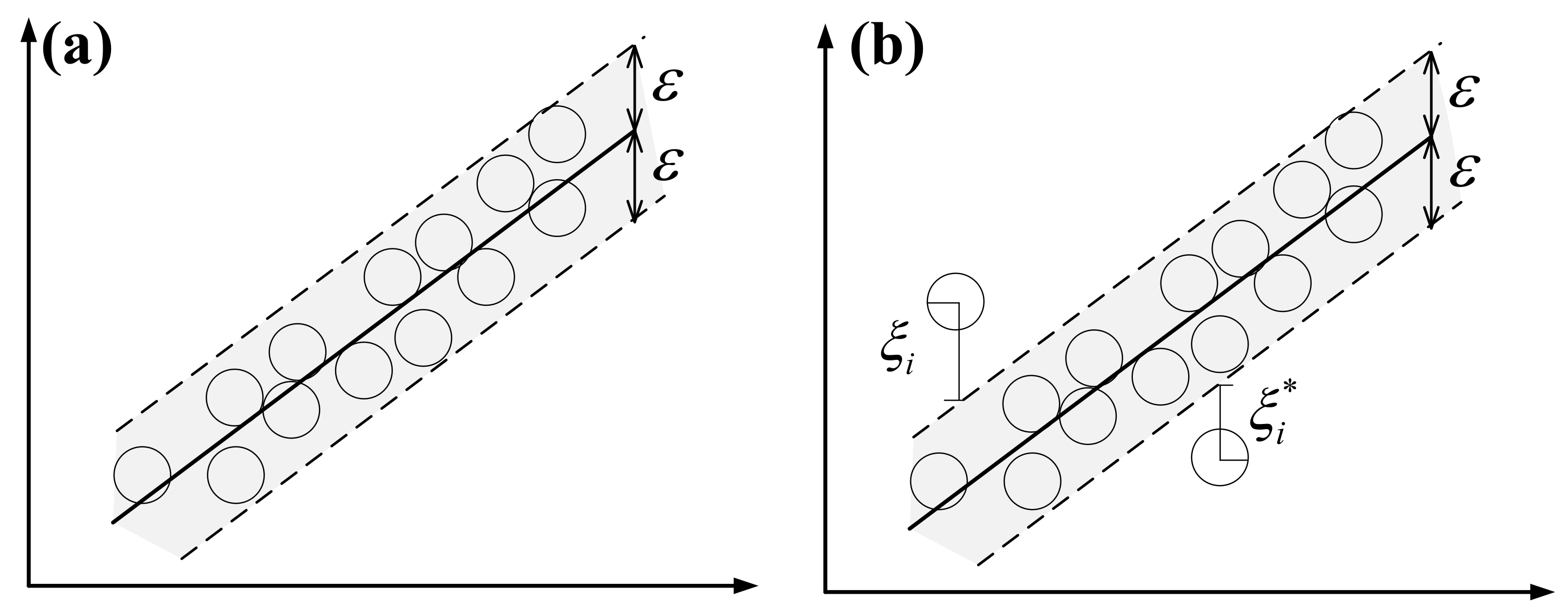
SVR regression is an adaptation of the support vector machine (SVM) algorithm used for regression problems [60]. The SVR can be divided into two types, i.e., hard margin and soft margin [61]. To illustrate the basic idea behind the SVR, we first introduce the case of linear functions, as shown in Figure 7a,b. In the hard margin model, there are no points outside the shaded region; the parameter $\epsilon$ affects the number of support vectors used in the regression function. That is, the smaller the value of $\epsilon$, the greater the number of support vectors that will be selected. However, this may not be the case, or we may also want to allow for some errors, as shown in Figure 7b; therefore, the soft margin SVR model was proposed. In the soft margin model, another important parameter, the cost parameter (C), is involved; it determines the tolerance for deviations larger than $\epsilon$ from the real value. That is, smaller deviations are tolerable for larger values of C. The training process of SVR is mathematically equivalent to the following optimization problem:

Minimize:

$$\frac{1}{2}{∥\mathbf{w}∥}^2+C\sum _{i=1}^n\left({\xi }_i+{\xi }_i^{*}\right)$$

(6)

Subject to:

$$\left\{\begin{array}{c}{y}_i-\mathbf{w}·\mathbf{x}-b⩽\epsilon +{\xi }_i\hfill \\ b+\mathbf{w}·\mathbf{x}-y_i⩽\epsilon +{\xi }_i^{*}\hfill \\ {\xi }_i,{\xi }_i^{*}⩾0\hfill \end{array}\right.$$

(7)

where C is the cost parameter and $C\ge 0$. $\mathbf{w}$ is the coefficient matrix.

The SVR formulations described above make up a linear decision boundary to fit the training dataset. Kernel functions are commonly used for non-linear SVR; they transform the data into a higher-dimensional feature space to enable linear fitting. There are two commonly used kernel functions, the polynomial and Gaussian radial basic functions.

The SVR can be used to estimate missing values by fitting an SVR to predict the non-missing values of $X_s$, i.e., $y_{obs}^{\left(s\right)}$∼$x_{obs}^{\left(s\right)}$, and using this to predict the missing values of $X_s$, i.e., $y_{mis}^{\left(s\right)}$∼$x_{mis}^{\left(s\right)}$. The SVR imputation algorithm is similar to RF.

4.3.3. ANN Imputation Method

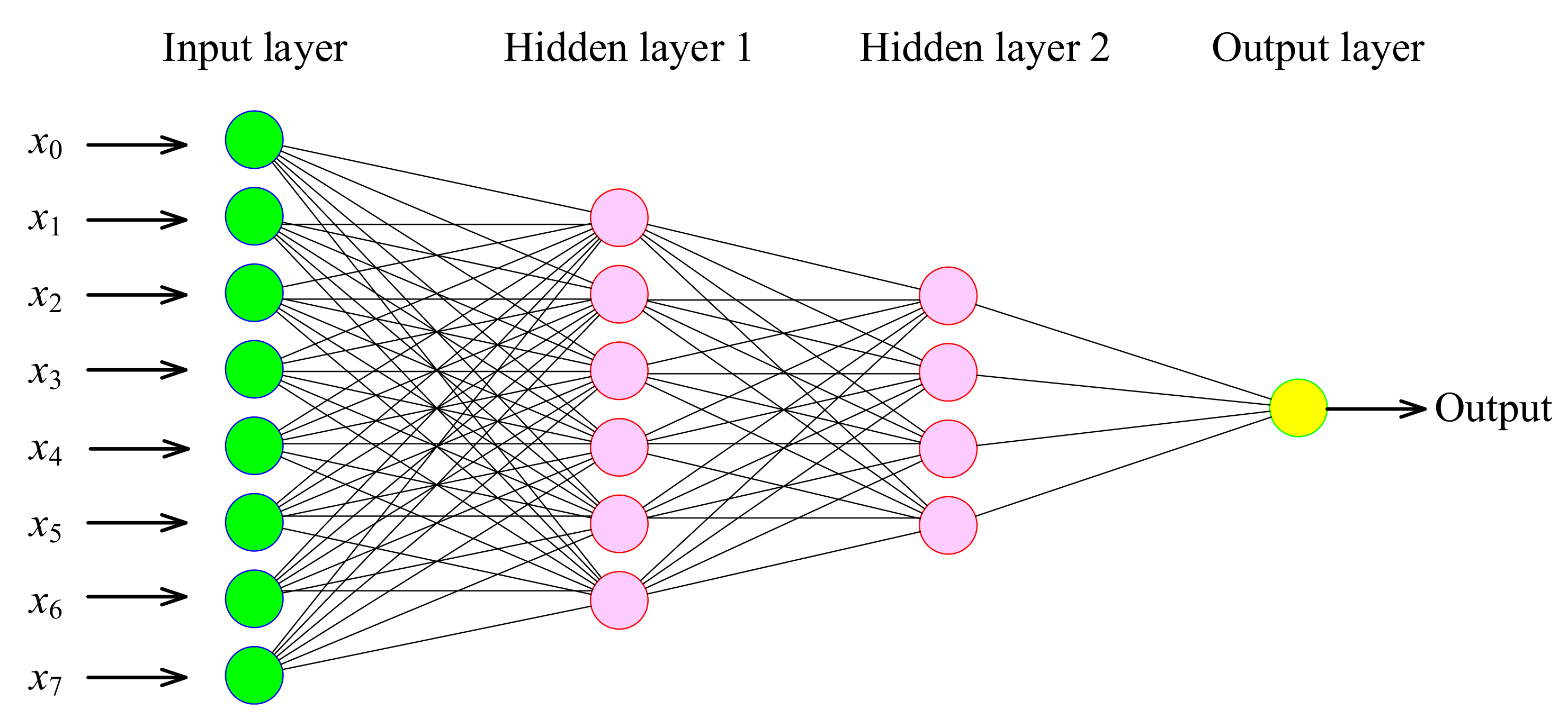
An artificial neural network (ANN) is a computing system designed to simulate the way that the human brain analyzes and processes information. It is the foundation of artificial intelligence and solves problems that would prove impossible or difficult by human or statistical methods. Feed-forward multi-layer perceptron ANNs are frequently used in engineering applications [62], as shown in Figure 8. Here, we use a standard ANN with one hidden layer as an example. Weights of the first layer connect the input data variables to the H hidden units (neurons), and the second layer’s weights connect these hidden neurons to the output units. First, given a p dimensional input vector $\mathbf{x}$, the H hidden neuron outputs are computed in the form [44]:

$$z_h=\sigma \left(\sum _{j=1}^p{w}_{hj}^{\left(1\right)}{x}_j+w_{h0}^{\left(1\right)}\right)$$

(8)

where $h=1,2,...,H$, $z_h$ is the hidden neuron output, $w_{hj}^{\left(1\right)}$ is the first layer weight, $w_{h0}^{\left(1\right)}$ is the corresponding bias parameter, the superscript (1) indicates that the corresponding parameters are in the first layer, and $\sigma$ is the activation function chosen as the ReLU function in this study. By analogy, considering $z_h$ as another input, the output can be calculated.

The ANN can be used to estimate missing values by fitting an ANN to predict the non-missing values of Xs, i.e., $y_{obs}^{\left(s\right)}$∼$x_{obs}^{\left(s\right)}$, and using this to predict the missing values of $X_s$, i.e., $y_{mis}^{\left(s\right)}$∼$x_{mis}^{\left(s\right)}$. The ANN imputation algorithm is also similar to RF.

5. Model Evaluation

5.1. Quantitative Evaluation

To assess the quality of the RF, SVR, ANN, mean, and MI predictions in the complete dataset (Dataset I), it was essential to establish metrics that allow the comparison of the different methods. This evaluation had to consist of a comparison between the prediction results and the actual results. We used two common statistical measurements, the root mean square error (RMSE) and the mean absolute error (MAE):

$$\mathrm{RMSE}=\sqrt{\frac{1}{n}\sum _{i=1}^n{\left(x_i-{\widehat{x}}_i\right)}^2}$$

(9)

$$\mathrm{MAE}=\frac{1}{n}\sum _{i=1}^n\left|x_i-{\widehat{x}}_i\right|$$

(10)

where $x_i$ is the actual value, ${\widehat{x}}_i$ is the predicted value, and n is the total number of missing value.

5.2. Qualitative Evaluation

RMSE and MAE of the imputation should also be used to determine which method performs better for imputing the missing values in UNSODA. However, the real values of these missing values are unknown, and we therefore used nonparametric tests (the reasons for not using ANOVA follow) to analyze whether there were any statistically significant differences between different features before and after imputation. As the missing values in UNSODA are supposed to be MAR, the data before and after the imputation were expected to not show significant differences. Before the ANOVA analysis, all features before and after imputation had to be tested for normality. In this study, the values of skewness and kurtosis were used. In addition, we used a multiple linear regression model to quantitatively determine which imputation method performed better for UNSODA.

6. Parameter Determination and Sensitivity Analysis

In this study, scikit-learn (version: 0.22), an open-source machine learning library, was used to perform the model training. We took the RF as an example to explain how to calibrate the parameters.

As discussed in Section 4.3.1, RF is a meta estimator that fits a number of CARTs on various sub-samples of the dataset and uses averaging to improve the predictive accuracy and control over-fitting.

The main parameters include the number of trees in the forest (n_estimators), the maximum depth of the tree (max_depth), and the minimum number of samples required to split an internal node (min_samples_split, default = 2). It should be noted that the number of features and sample sizes in Datasets I and II were not enough; therefore, the maximum depth of the tree was considered to be none, which meant nodes were expanded until all leaves were pure or until all leaves contained less than min_samples_split samples.

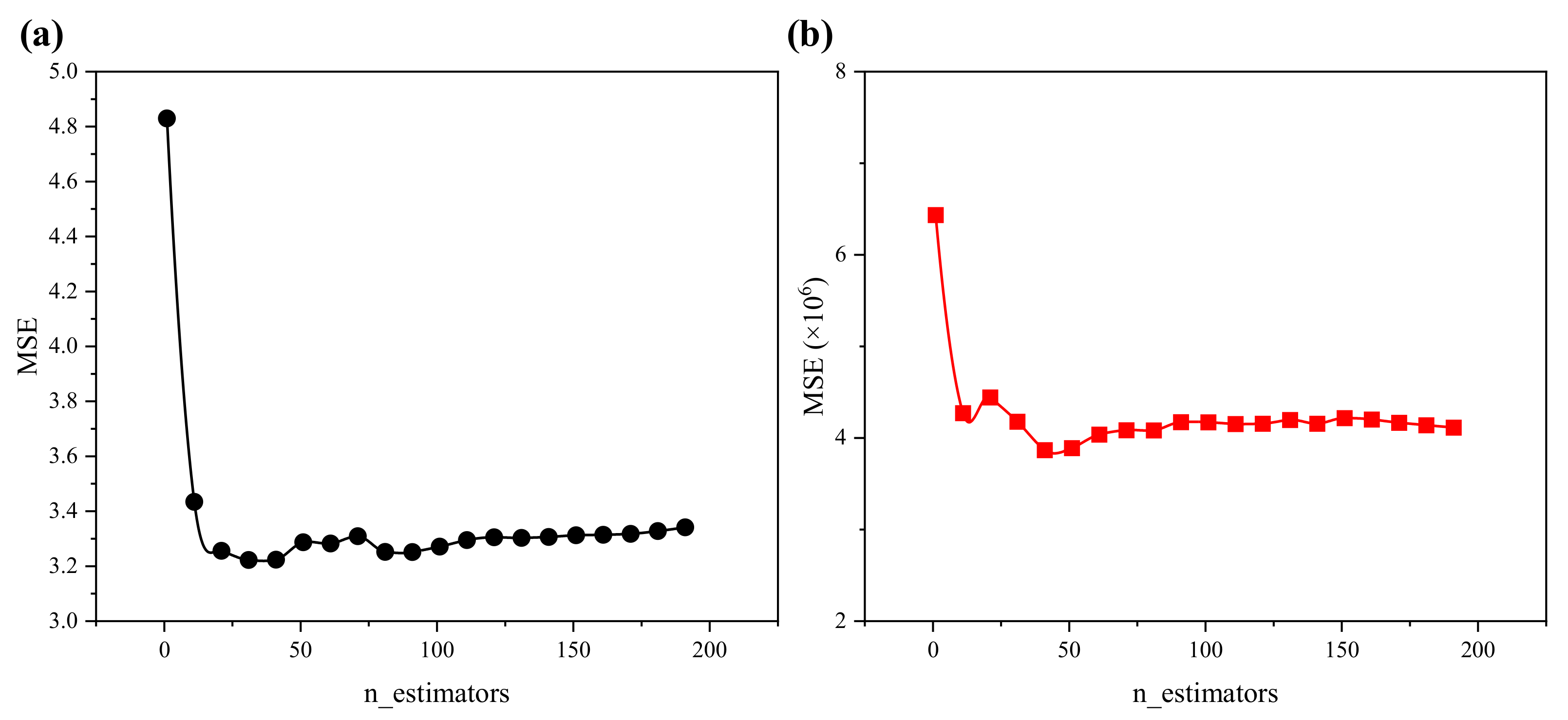
According to Bisong [63] and Pham et al. [64], the number of trees in the forest has a significant effect on the model accuracy and the RF will converge to a lower generalization error as the number of trees increases. Dataset I with a missing proportion = 0.15 was used to estimate the number of trees. As shown in Figure 9, the mean squared errors (MSEs) of pH and SHC did not decline when the numbers of trees exceeded 31 and 41, respectively. However, considering the size of the sample and the number of features, the n_estimators were considered to be 100. By analogy, the parameters of the SVR and ANN can be calibrated; the details are listed in

Table 3. Parameters used for model training.

Imputation Methods	Parameters
RF	n_estimators
	100
SVR	C	$\epsilon$	kernel
	100 (50)	0.01	rbf
ANN	learning_rate_init	activation	solver	alpha
	0.005 (0.06)	relu	adam	0.001 (1)

Note: the value in the round brackets used for Dataset II.

.

7. Results

7.1. Quantitative Measures for Dataset I

Table 4. Statistical measurements for RF, SVR, ANN, mean, and MI imputations in Dataset I.

Feature	Missing Proportion	RMSE RF	SVR	ANN	Mean	MI	MAE RF	SVR	ANN	Mean	MI
DU	0.03	5.99	15.39	32.2	26.68	5.5	6.61	16.17	39.28	23.27	4.8
	0.07	12.39	24.74	16.12	36.57	17.68	10.32	21.43	11.57	32	14.2
	0.11	33.32	39.23	34.2	40.24	28.19	19.8	27.78	18.93	29.06	21.8
	0.15	20.98	40.91	18.23	39.81	23.82	12.07	32.42	15	31.71	16.55
	0.19	25.58	42.73	45.38	64.12	44.16	17.07	32.43	38.88	49.03	30.62
	0.23	25.91	37.49	20.4	44.6	21.98	16.87	30.03	15.09	36.83	17.08
DL	0.03	6.43	23.72	59.07	40.9	15.57	5.36	20.81	43.67	34.97	9.93
	0.07	19.3	57	28.89	69.87	51.48	15.26	39.6	23.43	51.66	42.44
	0.11	33.26	34.85	42.43	42.29	54.19	21.54	27.27	32.77	36.79	46.8
	0.15	35.75	67.96	38.1	70.98	63.37	21.34	47.33	25.55	52.49	42.68
	0.19	26.54	28.76	61.14	31.64	44.12	17.57	21.65	42.71	27.82	32.73
	0.23	36.56	52.57	34.76	54.58	49.47	24.57	36.55	26.23	39.99	37.49
pH	0.03	0.86	0.91	0.32	1.32	1.08	0.81	0.8	0.27	1.29	0.83
	0.07	1.32	1.02	2.11	1.46	1.53	1.16	0.92	1.66	1.27	1.39
	0.11	1.86	1.69	2	1.61	1.88	1.76	1.49	1.82	1.53	1.57
	0.15	1.35	1.27	1.33	1.35	0.97	1.01	0.98	1	1.17	0.78
	0.19	1.65	1.98	1.95	1.66	1.71	1.43	1.71	1.65	1.51	1.51
	0.23	1.66	1.98	2.16	1.77	1.91	1.39	1.69	1.77	1.63	1.75
SHC	0.03	854.75	825.83	1200.1	662.66	953.15	679.27	519.22	935.43	576.29	751.7
	0.07	2818.95	3867.88	1710.57	3756.35	1887.4	1236.26	1256.13	751.89	1560.21	736.49
	0.11	1594.87	1906.36	1026.96	1839.52	303.95	710.16	582.82	563.94	901.18	202.68
	0.15	1896.67	1951.17	1697.06	1867.5	1933.28	682.14	630.66	984.73	903.6	738.41
	0.19	2299.21	2986.01	1794.31	2867.45	2003.19	1098.22	995.45	852.43	1252.13	790.91
	0.23	1264.22	938.44	1328.83	899.61	879.01	717.31	384.24	805.91	674.99	428.77
OMC	0.03	0.69	0.64	3.65	1.78	0.76	0.48	0.53	2.96	1.78	0.53
	0.07	1.78	1.83	1.7	2.51	1.37	1.36	1.32	1.01	2.15	1.24
	0.11	0.49	1.37	0.97	1.52	1.14	0.45	1.02	0.8	1.41	0.88
	0.15	1.69	1.86	3.28	1.98	1.97	0.84	1.35	2.13	1.69	1.21
	0.19	1.7	1.45	2.19	2	2.07	0.92	1.06	1.32	1.8	1.37
	0.23	1.35	1.4	2.75	1.7	1.58	0.91	1.06	1.64	1.63	1.1
PO	0.03	0.005	0.101	0.18	0.077	0.002	0.005	0.061	0.128	0.059	0.002
	0.07	0.017	0.077	0.057	0.088	0.011	0.013	0.059	0.051	0.072	0.005
	0.11	0.01	0.074	0.083	0.074	0.004	0.008	0.064	0.075	0.064	0.004
	0.15	0.023	0.199	0.088	0.09	0.016	0.014	0.117	0.062	0.065	0.011
	0.19	0.015	0.065	0.13	0.065	0.019	0.013	0.056	0.097	0.051	0.012
	0.23	0.008	0.056	0.131	0.057	0.007	0.007	0.046	0.103	0.045	0.004
PD	0.03	0.09	0.1	0.17	0.03	0.02	0.07	0.07	0.16	0.02	0.02
	0.07	0.09	0.05	0.22	0.06	0.03	0.06	0.04	0.19	0.05	0.02
	0.11	0.06	0.05	0.13	0.11	0.02	0.05	0.04	0.1	0.06	0.02
	0.15	0.2	0.2	0.25	0.21	0.1	0.11	0.12	0.17	0.12	0.05
	0.19	0.06	0.05	0.26	0.07	0.08	0.05	0.04	0.22	0.05	0.05
	0.23	0.05	0.08	0.24	0.09	0.03	0.05	0.06	0.19	0.07	0.02

summarizes statistical measurements for the performances of RF, SVR, ANN, mean, and MI methods on Dataset I. The obtained results revealed that the missing proportion has a potential effect on the performances of the imputation methods. RF and MI outperformed the other imputation methods examined in this study; the mean and ANN had inferior performances.

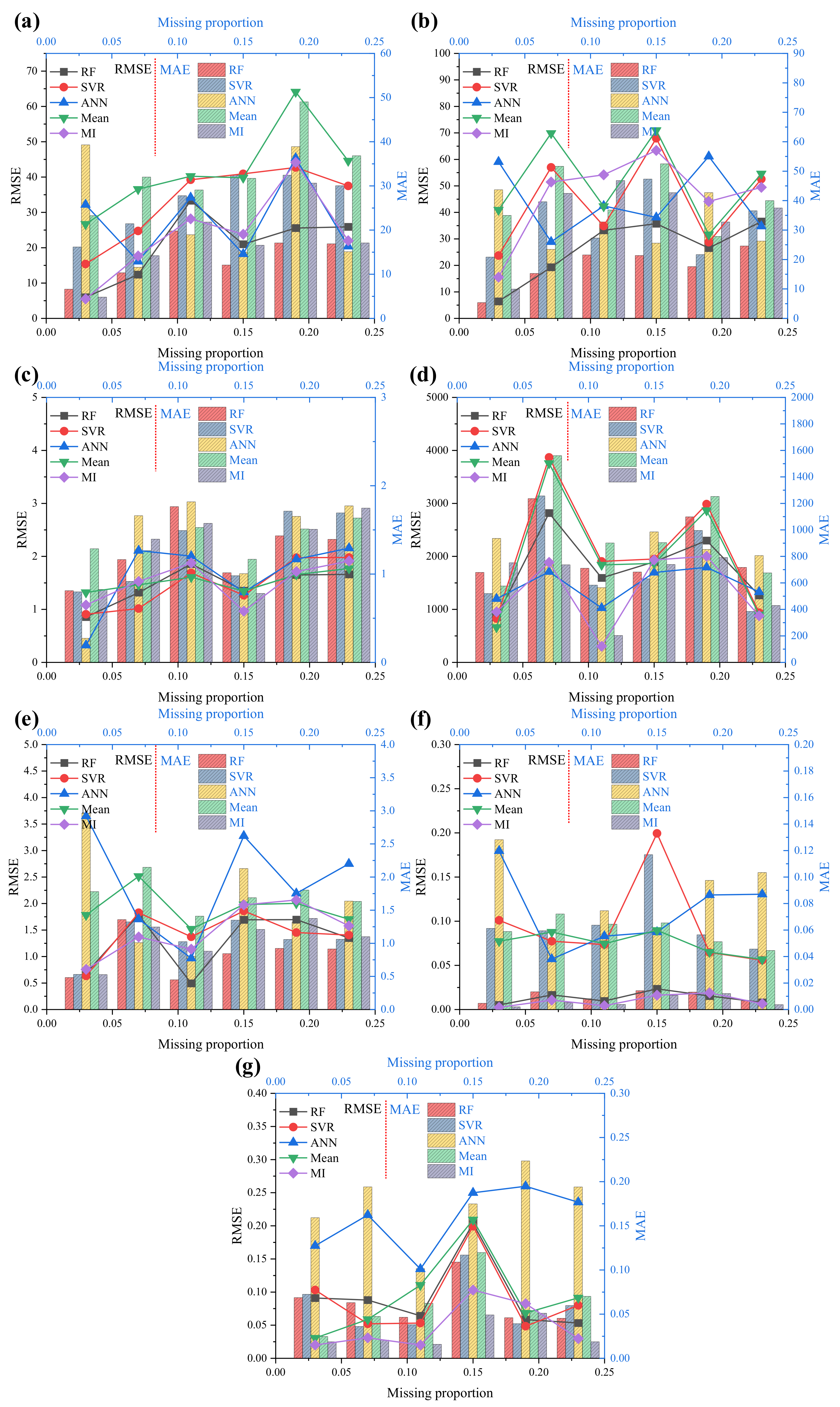
For further discussions, Figure 10 presents the relationship between the missing proportion and the statistical measurements for each imputation method. For RF imputation, when the missing proportion increased from 0.03 to 0.11, the RMSE of the DU increased from 5.99 to 33.32, and the MAE increased from 6.61 to 19.80. However, when the missing proportion increased from 0.11 to 0.15, the RMSE was decreased significantly from 33.32 to 20.98, and the MAE from 19.80 to 12.07. When the missing proportion further increased from 0.15 to 0.23, the RMSE increased from 20.98 to 25.91, and the MAE from 12.07 to 16.87. Similar behavior was obtained for DL, pH, SHC, OMC, PO, and PD.

For SVR imputation, when the missing proportion increased from 0.03 to 0.19, the RMSE of the DU increased from 15.39 to 42.73, and the MAE increased from 16.17 to 32.43. However, when the missing proportion increased from 0.19 to 0.23, the RMSE was gradually reduced from 42.73 to 37.49, and the MAE decreased from 32.43 to 30.3. Similar behavior was obtained for DL, pH, SHC, OMC, PO, and PD. The ANN, mean, and MI imputations performed similarly to the RF and SVR imputations.

The above discussion cannot clearly explain which methods performed better for Dataset I, because the RMSEs and MAEs of all features fluctuated within accepted ranges, except for SHC. It should be noted that the RMSE and MAE of SHC were high using every imputation method, probably because of the outliers in the raw data, as shown in Figure 3d. These results indicate that RF, SVR, ANN, mean, and MI methods are adequate and could be used to impute the missing values in the original incomplete dataset (Dataset II).

7.2. Qualitative Measures for Dataset II

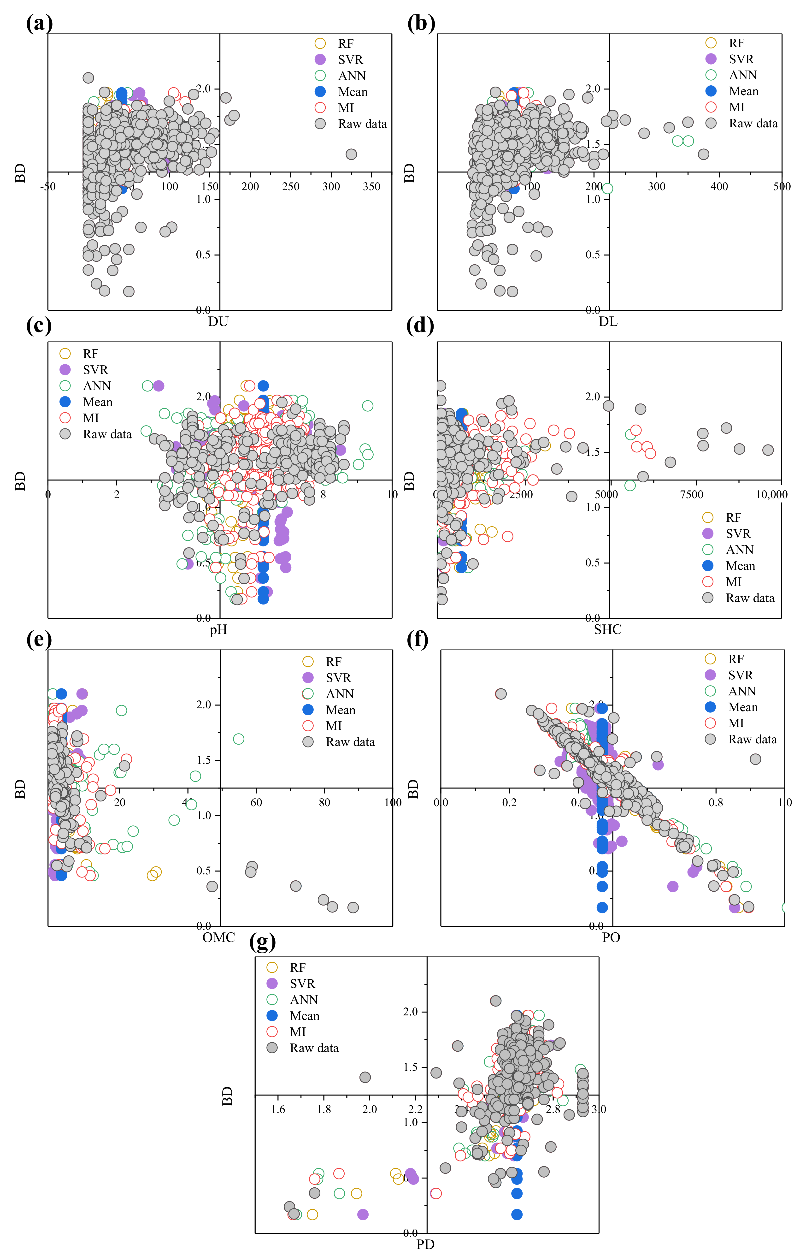
After imputing missing values in dataset II, we took the features (or independent variables) DU, DL, pH, SHC, OMC, PO, and PD as the x-axis variables, and the label (or dependent variable) BD as the y-axis variable. We also assumed that XXR referred to the feature after RF imputation, XXS to the feature after SVR imputation, XXA to the feature after ANN imputation, XXM to the feature after mean imputation, XXMI to the feature after MI imputation, and XXO to the feature before imputation (i.e., the raw data).

Figure 11 shows the distributions of DU, DL, pH, SHC, OMC, PO, and PD before and after imputation. The results demonstrate that the data for each feature were distributed well in the major quadrants after RF, SVR, ANN, mean, and MI, indicating that these imputation methods are feasible. The sample size, minimum value, maximum value, mean value, standard deviation, and standard error; and the median, skewness, kurtosis, coefficient of variation, and variance of each feature before and after imputation are listed in

Table 5. The basic information of the features before and after imputation.

Feature	Name	Sample Size	Min	Max	Mean	Standard Deviation	Standard Error	Median	Kurtosis	Skewness	Coefficient of Variation	Variance
DU	DUO	659	0	325	41.231	40.316	1.57	30	3.517	1.357	97.78%	1625.378
	DUR	762	0	325	39.736	37.752	1.368	30	4.562	1.541	95.01%	1425.22
	DUS	762	0	325	40.704	37.85	1.371	33.205	4.348	1.473	92.99%	1432.658
	DUA	762	0	325	41.234	37.936	1.374	35	4.258	1.441	92.00%	1439.103
	DUM	762	0	325	41.231	37.488	1.358	40	4.532	1.459	90.92%	1405.386
	DUMI	762	0	325	41.701	38.497	1.395	33	3.79	1.351	92.32%	1482.011
DL	DLO	659	6	3000	72.466	124.601	4.854	56	464.535	19.855	171.94%	15,525.368
	DLR	762	6	3000	70.533	116.087	4.205	57.21	534.314	21.27	164.59%	13,476.125
	DLS	762	6	3000	70.87	116.049	4.204	55.284	534.77	21.283	163.75%	13,467.300
	DLA	762	6	3000	79.92	155.859	5.646	60	213.387	13.278	195.02%	24,291.898
	DLM	762	6	3000	72.466	115.862	4.197	65	537.058	21.344	159.89%	13,424.037
	DLMI	762	6	3000	71.48	116.176	4.209	59.9	531.973	21.197	162.53%	13,496.809
pH	pHO	279	3.1	8.6	6.259	1.513	0.091	6.7	−1.219	−0.355	24.17%	2.288
	pHR	762	3.1	8.6	6.298	1.039	0.038	6.441	0.176	−0.526	16.49%	1.079
	pHS	762	3.1	8.6	6.407	1.104	0.04	6.744	0.182	−0.846	17.23%	1.219
	pHA	762	2.857	10.413	6.178	1.185	0.043	6.334	−0.056	−0.24	19.19%	1.405
	pHM	762	3.1	8.6	6.259	0.914	0.033	6.259	1.884	−0.584	14.61%	0.836
	pHMI	762	3.1	8.6	6.29	1.064	0.039	6.36	0.027	−0.484	16.91%	1.131
SHC	SHCO	425	0.019	27,648	613.559	1935.074	93.865	95.9	97.723	8.448	315.39%	3,744,509.62
	SHCR	762	0.019	27,648	540.376	1472.962	53.36	229.387	165.31	10.812	272.58%	2,169,617.99
	SHCS	762	0.019	27,648	384.797	1467.129	53.148	96.737	172.699	11.23	381.27%	2,152,468.57
	SHCA	762	0.019	27,648	501.111	1501.694	54.401	135.307	154.204	10.371	299.67%	2,255,085.69
	SHCM	762	0.019	27,648	613.559	1444.402	52.325	613.559	176.677	11.294	235.41%	2,086,297.08
	SHCMI	762	0.019	27,648	619.756	1585.248	57.427	207.092	122.024	8.941	255.79%	2,513,012.29
OMC	OMCO	367	0.01	88.4	2.942	9.727	0.508	0.94	50.679	6.976	330.61%	94.611
	OMCR	762	0.01	88.4	2.217	7.01	0.254	0.958	96.343	9.395	316.15%	49.147
	OMCS	762	−0.732	88.4	1.953	6.864	0.249	0.92	105.92	9.946	351.45%	47.111
	OMCA	762	0.01	88.4	2.824	7.794	0.282	1.128	64.553	7.507	276.01%	60.742
	OMCM	762	0.01	88.4	2.942	6.746	0.244	2.942	107.704	10.031	229.28%	45.503
	OMCMI	762	0.01	88.4	2.48	7.459	0.27	1.116	84.869	8.843	300.78%	55.642
PO	POO	366	0.175	0.915	0.469	0.104	0.005	0.456	3.001	1.298	22.08%	0.011
	POR	762	0.175	0.915	0.456	0.091	0.003	0.442	4.52	1.598	20.02%	0.008
	POS	762	0.175	0.915	0.464	0.077	0.003	0.458	8.156	1.989	16.66%	0.006
	POA	762	0.175	1.008	0.468	0.091	0.003	0.448	5.628	1.8	19.50%	0.008
	POM	762	0.175	0.915	0.469	0.072	0.003	0.469	9.445	1.869	15.29%	0.005
	POMI	762	0.174	0.915	0.457	0.092	0.003	0.444	4.489	1.593	20.05%	0.008
PD	PDO	395	1.65	2.93	2.642	0.126	0.006	2.65	26.025	−3.401	4.76%	0.016
	PDR	762	1.65	2.93	2.644	0.106	0.004	2.652	37.489	−4.462	4.01%	0.011
	PDS	762	1.65	2.93	2.642	0.099	0.004	2.648	40.998	−4.4	3.73%	0.01
	PDA	762	1.65	2.93	2.639	0.116	0.004	2.65	34.429	−4.43	4.40%	0.013
	PDM	762	1.65	2.93	2.642	0.091	0.003	2.642	52.684	−4.716	3.43%	0.008
	PDMI	762	1.65	2.93	2.644	0.113	0.004	2.65	36.35	−4.484	4.26%	0.013

. The mean value was computed from the sample data. It should be noted that the standard deviation differs from the standard error: the standard deviation indicates approximately how far individuals are from the mean values, whereas the standard error estimates the variability of the sample mean—i.e., approximately how far it is from the population mean [65].

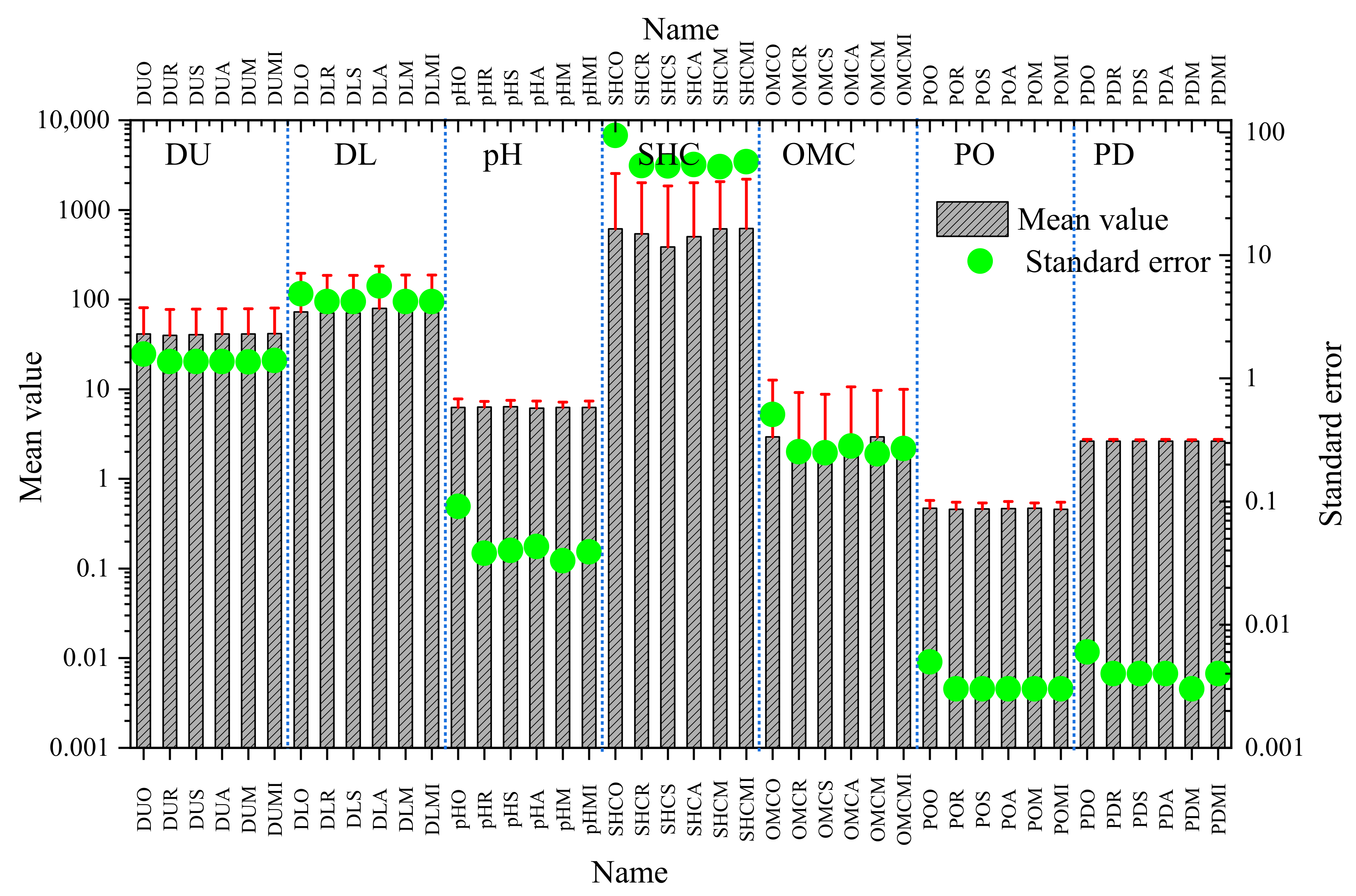
Table 5 shows that the standard errors of DU, DL, pH, SHC, OMC, PO, and PD decreased from 1.570, 4.854, 0.091, 93.865, 0.508, 0.005, and 0.006 to 1.368, 4.205, 0.038, 53.360, 0.254, 0.003, and 0.004 after RF imputation; to 1.371, 4.204, 0.040, 53.148, 0.249, 0.003, and 0.004 after SVR imputation; to 1.374, 5.646, 0.043, 54.401, 0.282, 0.003, and 0.004 after ANN imputation, to 1.358, 4.197, 0.033, 52.325, 0.244, 0.003, and 0.003 after mean imputation; and to 1.395, 4.209, 0.039, 57.427, 0.270, 0.003, and 0.004 after MI imputation, indicating that the sample means became closer to the population means. The decreased coefficients of variation and standard deviations indicated that individuals were closer to the sample mean values.

Table 5 also shows that the maximum values of DUO, DLO, SHCO, and OMCO were three standard deviations away from the mean values; and the maximum values of DUR, DUS, DUA, DLR, DLS, DLA, SHCR, SHCS, SHCA, OMCR, OMCS, OMCA, DUM, DLM, SHCM, OMCM, DUMI, DLMI, SHCMI, and OMCMI were still three standard deviations away from the mean values, indicating that the raw data fluctuate greatly. To more clearly visualize this finding, the means, standard deviations, and standard errors for all features before and after imputation are plotted in Figure 12.

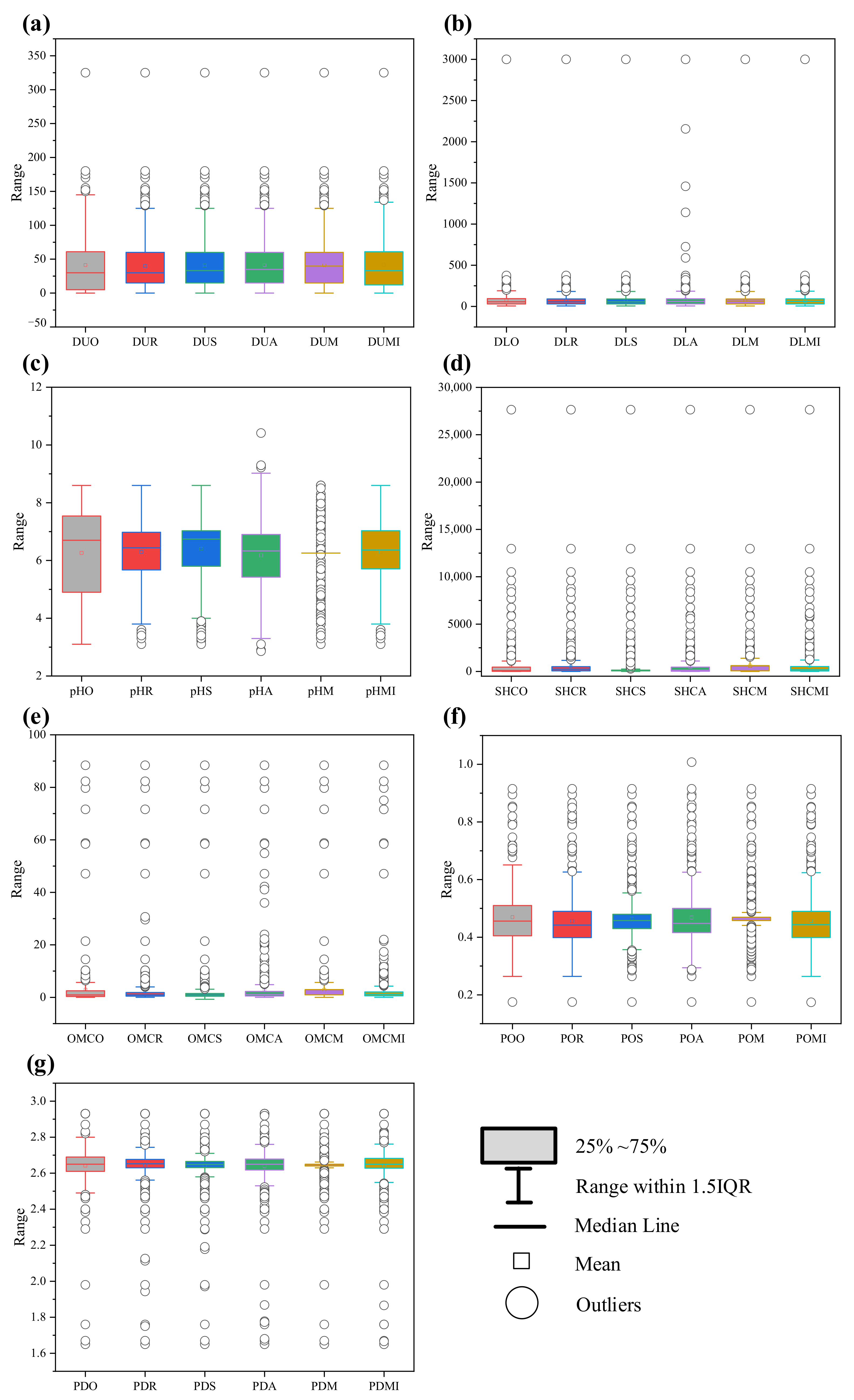
Figure 13 presents the boxplots for the DU, DL, pH, SHC, OMC, PO, and PD before and after mean, MI, RF, SVR, and ANN imputation. The statistical descriptions indicate that the same features lay within the same scales. Among them, the SHC still had the broadest range, i.e., 0.019–27,648, in which the distribution was mostly skewed toward the low value in the range from 60.415 to 512.541 after RF imputation; 61.836 to 144.250 after SVR imputation; 22.722 to 455.400 after ANN imputation; 69.600 to 613.559 after mean imputation; 53.272 to 518.500 after MI imputation. On the other hand, the distribution ratio of PO had the narrowest range, i.e., 0.174–0.915, which centered in the range of 0.399–0.490 after RF imputation; 0.430–0.480 after SVR imputation; 0.416–0.500 after ANN imputation; 0.458–0.469 after mean imputation; 0.399 to 0.491 after MI imputation. Figure 13 also shows that mean imputations generated many outliers, such as for pH and PO, which shows that the mean imputation cannot be used for pH and PO. It is worth noting that ANN imputation also generated outliers for DL.

Skewness measures the relative symmetry of a distribution, and a value of zero indicates symmetry. The larger the absolute value of skewness, the more asymmetric the distribution. A positive value indicates a long right tail, and a negative value indicates a long left tail. By contrast, kurtosis measures the relative peakedness. The values of skewness and kurtosis for DUO, DUR, DUS, DUA, DUM, DUMI, DLO, DLR, DLS, DLA, DLM, DLMI, pHO, pHR, pHS, pHA, pHM, pHMI, SHCO, SHCR, SHCS, SCHA, SHCM, SHCMI, OMCO, OMCR, OMCS, OMCA, OMCM, OMCMI, POO, POR, POS, POA, POM, POMI, PDO, PDR, PDS, PDA, PDM, and PDMI are also listed in Table 5. All of these features did not strictly meet the criterion for normality. Therefore, nonparametric tests rather than ANOVA were used to investigate whether there were differences before and after imputation, and the results are listed in

Table 6. Nonparametric test results.

Feature	Median($\mathit{Q}25$,$\mathit{Q}75$)		MannWhitney U	MannWhitney z	p	Feature	Median ($\mathit{Q}25$,$\mathit{Q}75$)		MannWhitney U	MannWhitney z	p
DU	Raw data (n = 659)	RF (n = 762)	250,299.5	−0.101	0.919		Raw data (n = 425)	Mean (n = 762)	116,598.5	−8.098	0.000 **
	30.000(5.0,61.0)	30.000(15.0,60.0)				SHC	95.900(20.8,459.4)	613.559(69.6,613.6)
		SVR (n = 762)	247,602.5	−0.453	0.651			MI (n = 762)	135,141.5	−4.73	0.000 **
		33.205(15.0,60.0)						207.092(53.3,518.5)
		ANN (n = 762)	245,348.5	−0.746	0.456		Raw data (n = 367)	RF (n = 762)	137,024	−0.546	0.585
		35.000(15.0,60.0)					0.940(0.3,2.5)	0.958(0.5,1.9)
		Mean (n = 762)	243,611.5	−0.973	0.331			SVR (n = 762)	132,498.5	−1.428	0.153
		40.000(15.0,60.0)						0.920(0.4,1.5)
		MI (n = 762)	245,028	−0.788	0.431	OMC		ANN (n = 762)	126,483.5	−2.6	0.009 **
		33.000(12.0,61.0)						1.128(0.5,2.3)
DL	Raw data (n = 659)	RF (n = 762)	250,327.5	−0.097	0.922			Mean (n = 762)	97,759.5	−8.379	0.000 **
	56.000(30.0,95.0)	57.210(30.0,91.0)						2.942(1.0,2.9)
		SVR (n = 762)	249,248.5	−0.237	0.812			MI (n = 762)	127,130.5	−2.474	0.013 *
		55.284(30.0,91.0)						1.116(0.6,2.1)
		ANN (n = 762)	246,019.5	−0.656	0.512		Raw data (n = 366)	RF (n = 762)	128,268	−2.182	0.029 *
		60.000(30.0,93.0)					0.456(0.4,0.5)	0.442(0.4,0.5)
		Mean (n = 762)	243,199.5	−1.022	0.307			SVR (n = 762)	137,856	−0.31	0.756
		65.000(30.0,91.0)						0.458(0.4,0.5)
		MI (n = 762)	247,989	−0.401	0.689	PO		ANN (n = 762)	139,339	−0.021	0.983
		59.900(30.0,92.0)						0.448(0.4,0.5)
pH	Raw data (n = 279)	RF (n = 762)	100,975.5	−1.239	0.215			Mean (n = 762)	128,358	−2.213	0.027 *
	6.700(4.9,7.5)	6.441(5.7,7.0)						0.469(0.5,0.5)
		SVR (n = 762)	104,703.5	−0.371	0.71			MI (n = 762)	128,777.5	−2.083	0.037 *
		6.744(5.8,7.0)						0.444(0.4,0.5)
		ANN (n = 762)	97,681.5	−2.006	0.045 *		Raw data (n = 395)	RF (n = 762)	140,712	−1.817	0.069
		6.334(5.4,6.9)					2.650(2.6,2.7)	2.652(2.6,2.7)
		Mean (n = 762)	96,880.5	−2.311	0.021 *			SVR (n = 762)	148,596.5	−0.353	0.724
		6.259(6.3,6.3)						2.648(2.6,2.7)
		MI (n = 762)	101,044.5	−1.223	0.221	PD		ANN (n = 762)	149,471.5	−0.19	0.849
		6.360(5.7,7.0)						2.650(2.6,2.7)
SHC	Raw data (n = 425)	RF (n = 762)	134,844.5	−4.783	0.000 **			Mean (n = 762)	148,109.5	−0.45	0.653
	95.900(20.8,459.4)	229.387(60.4,512.5)						2.642(2.6,2.6)
		SVR (n = 762)	161,420.5	−0.089	0.929			MI (n = 762)	144,380	−1.136	0.256
		96.737(61.8,144.3)						2.650(2.6,2.7)
		ANN (n = 762)	156,553.5	−0.949	0.343
		135.307(22.7,455.4)

* p < 0.05 ** p < 0.01.

.

Table 6 suggests that there were no significant differences before and after imputation, except for SHCO and SHCR, SHCO and SHCM, SHCO and SHCMI, POO and POR, POO and POM, POO and POMI, pHO and pHA, pHO and pHM, OMCO and OMCA, OMCO and OMCM, and OMCO and OMCMI. As discussed above, this result may have been caused by the raw data. Although there was a difference in SHC and PO before and after RF imputation, we assume that the RF imputation is still valid based on observations of the mean and median. The pH and OMC metrics before and after ANN imputation are similar.

After nonparametric tests, we used a multiple linear regression model to quantitatively determine which imputation method performed better for UNSODA. In the multiple linear regression model, DU, DL, pH, SHC, OMC, PO, and PD were still considered to be independent and BD dependent. However, it should be noted that DU and DL are collinear. Therefore, we should consider only one feature, and DU was used in this study. For comparison, multiple linear regression was also performed for these features when missing data were imputed by zero.

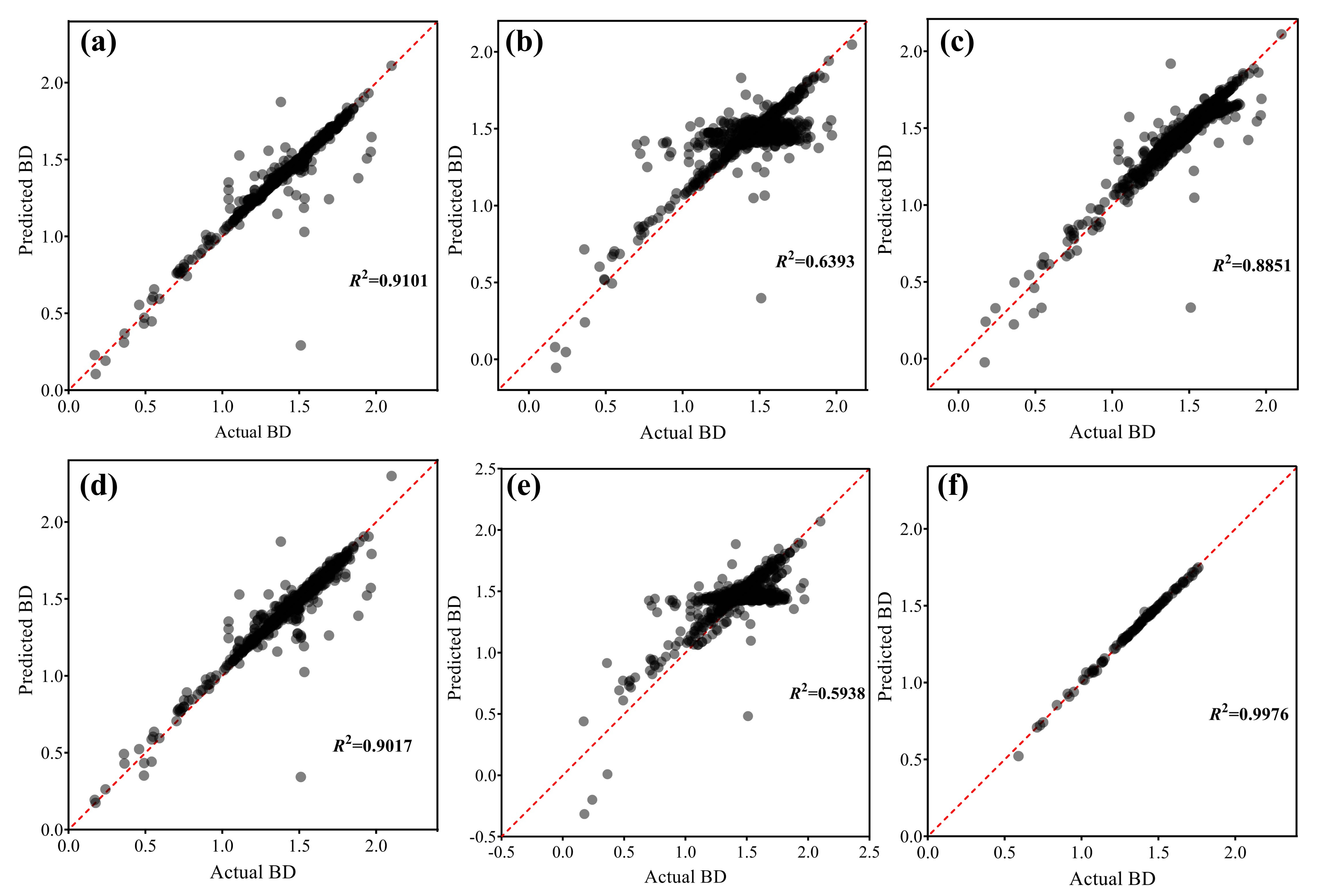
The results of multiple linear regression after RF, SVR, ANN, mean, MI, and zero imputations are presented in

Table 7. Multilinear regression analysis results.

Imputation Method	Independent Variable	Unstandardized Coefficients		t	p	VIF	${\mathit{R}}^2$	Adj ${\mathit{R}}^2$	F
		B	Standard Error
RF	Constant	1.483	0.11	13.426	0.000 **	-	0.910	0.909	F(6,755) = 1273.712, p = 0.000
	DU	0	0	2.579	0.010 *	1.055
	pH	−0.001	0.003	−0.193	0.847	1.052
	SHC	0	0	−0.325	0.745	1.035
	OMC	0.002	0.001	2.849	0.005 **	2.899
	PO	−2.481	0.036	−68.031	0.000 **	1.472
	PD	0.41	0.041	10.106	0.000 **	2.463
SVR	Constant	1.836	0.223	8.234	0.000 **	-	0.639	0.636	F(6,755) = 223.020, p = 0.000
	DU	0	0	−1.325	0.185	1.121
	pH	0.009	0.005	1.811	0.07	1.035
	SHC	0	0	0.659	0.51	1.064
	OMC	−0.003	0.001	−2.62	0.009 **	2.445
	PO	−2.322	0.085	−27.477	0.000 **	1.409
	PD	0.242	0.083	2.933	0.003 **	2.193
ANN	Constant	1.454	0.119	12.245	0.000 **	-	0.885	0.884	F(6,755) = 968.854, p = 0.000
	DU	0	0	−3.34	0.001 **	1.128
	pH	0.011	0.003	3.918	0.000 **	1.148
	SHC	0	0	−2.396	0.017 *	1.057
	OMC	0.003	0.001	4.78	0.000 **	3.123
	PO	−2.501	0.042	−58.998	0.000 **	1.554
	PD	0.416	0.045	9.319	0.000 **	2.79
Mean	Constant	2.633	0.215	12.226	0.000 **	-	0.594	0.591	F(6,755) = 183.955, p = 0.000
	DU	0	0	3.077	0.002 **	1.046
	pH	0.016	0.006	2.486	0.013 *	1.014
	SHC	0	0	−0.462	0.644	1.042
	OMC	−0.012	0.001	−11.496	0.000 **	1.376
	PO	−2.161	0.088	−24.682	0.000 **	1.159
	PD	−0.098	0.076	−1.293	0.197	1.382
MI	Constant	1.507	0.11	13.719	0.000**	-	0.902	0.901	F(6,755)=1154.513, p = 0.000
	DU	0	0	2.252	0.025 *	1.082
	pH	0.001	0.003	0.392	0.695	1.079
	SHC	0	0	−0.691	0.49	1.044
	OMC	0.003	0.001	4.179	0.000 **	2.772
	PO	−2.491	0.036	−69.058	0.000 **	1.325
	PD	0.399	0.042	9.59	0.000 **	2.66
Zero	Constant	1.48	0.013	112.448	0.000 **	-	0.379	0.374	F(6,755) = 76.715, p = 0.000
	DU	0.001	0	4.185	0.000 **	1.056
	pH	−0.001	0.002	−0.424	0.672	1.07
	SHC	0	0	4.029	0.000 **	1.021
	OMC	−0.016	0.001	−14.524	0.000 **	1.063
	PO	−0.493	0.049	−10.128	0.000 **	2.74
	PD	0.048	0.009	5.331	0.000 **	2.738
Discarding Missing values	Constant	1.069	0.04	26.925	0.000 **	-	0.998	0.997	F(6,102) = 6932.797, p = 0.000
	DU	0	0	2.027	0.045 *	1.341
	pH	−0.002	0.001	−2.084	0.040 *	1.076
	SHC	0	0	−2.762	0.007 **	2.747
	OMC	0.002	0.001	3.151	0.002 **	3.111
	PO	−2.551	0.019	−133.224	0.000 **	2.004
	PD	0.581	0.015	40.031	0.000 **	1.665

* p < 0.05 ** p < 0.01. Dependent variable: BD.

. Table 7 shows that $R^2$ was 0.910 for the RF imputation, which meant that DU, pH, SHC, OMC, PO, and PD could explain 91.0% of the variation in BD. The model passed the F-test (F = 1273.712, p = 0.000 < 0.05), indicating that at least one of DU, pH, SHC, OMC, PO, and PD affect BD, and the model’s formula was: BD = 1.483 + (0.000 × DU) − (0.001 × pH) + (0.000 × SHC) + (0.002 × OMC) − (2.481 × PO) + (0.410 × PD). A test for multicollinearity indicated that all the variance inflation factor (VIF) values in the model were less than five, which meant that there was no collinearity problem [66]. The results for SVR, ANN, mean, MI, and zero imputations were similar to those for RF imputation, but their $R^2$ values (0.639 for SVR imputation, 0.885 for ANN imputation, 0.594 for mean imputation, 0.902 for MI method, and 0.379 for zero imputation) were smaller. It should be noted that the $R^2$ value for MI imputation is close to those of the RF imputation method, and the model also passed the F-test (F = 1154.513, p = 0.000 < 0.05), indicating that the performance of the MI method was close to that of the RF imputation. We also considered the effect of discarding missing values, which decreased the number of datasets substantially (n = 109). The analysis results when missing values were discarded are presented in Table 7. The $R^2$ value was 0.998, which meant that DU, pH, SHC, OMC, PO, and PD could explain 99.8% of the variation in BD. This model still passed the F-test (F = 6932.797, p = 0.000 < 0.05), indicating that at least one of DU, pH, SHC, OMC, PO, and PD affect BD, and the model’s formula was: BD = 1.069 + (0.000 × DU) − (0.002 × pH) + (0.000 × SHC) + (0.002 × OMC) − (2.551 × PO) + (0.581 × PD). Although the $R^2$ values of the RF, SVR, and ANN imputation were smaller than those obtained after discarding missing values, the above discussion suggests that these imputation methods are feasible; and RF and MI methods may be better than SVR, ANN, mean, and zero imputation. The results of the actual BD and predicted BD are shown in Figure 14.

8. Discussion

The reason for using regression to impute the missing values is that the regression algorithm believes that there is some connection between the Eigen matrix and the label. That is, we can use features $X_1$, $X_2$, $X_3$, and $X_4$ to predict the label Y. Similarly, we can also use Y, $X_2$, $X_3$, and $X_4$ to predict $X_1$.

Before imputing the missing values in the original incomplete, Dataset I was simulated with different missing proportions (e.g., 3%, 7%, 11%, 15%, 19%, and 23%) using an MAR approach. It should be noted that the maximum simulated missing proportion was 23%, which is far below the average level of missing data in Dataset II. In fact, it would be difficult to simulate a high missing proportion considering the sample size of Dataset I. The main reason is the sample size of Dataset I is insufficient; the ANN imputation fails to converge with the increase of the missing proportion.

In this study, we mainly focused on the comparison of various methods of handling missing data in UNSODA. The imputed dataset was not used for modeling and applying in a case study. It will be more convincing if the quality of a real case study’s results can be improved after imputing the missing data using the proposed method. By observing multiple linear regression, we can infer that the data after RF and MI imputation can be used in a case study. We will use the imputed Dataset II to predict BD in the future according to PTFs proposed by Yi et al. [12], Curtis and Post [14], Adams [67] and Rawls [68].

In addition, the outliers were not deleted or replaced because of the imputation, which may have caused the large RMSEs and MAEs for SHC. In a subsequent study, we will further explore how to predict SHC well.

9. Conclusions

Three machine learning-based methods, i.e., random forest (RF) regression, support vector (SVR) regression, and artificial neural network (ANN) regression, and two statistics-based methods, i.e., mean and multiple imputation (MI) were used to impute the missing data for DU, DL, pH, SHC, OMC, PO, and PD in UNSODA. Both quantitative and qualitative methods were used to evaluate the feasibility. Based on the results, we can conclude that:

(1)

The RMSEs and MAEs of DU, DL, pH, SHC, OMC, PO, and PD for the complete dataset indicate that RF, SVR, ANN, mean, and MI methods are appropriate for imputing the missing values in UNSODA.

(2)

The standard error significantly decreased after imputation, indicating that the sample means had become closer to the population mean. The decreased coefficients of variation and standard deviations indicate that the individual data points were closer to the sample mean values.

(3)

There were no significant differences before and after imputation for DU, DL, pH, SHC, OMC, PO, and PD.

(4)

DU, pH, SHC, OMC, PO, and PD explained 91.0%, 63.9%, 88.5%, 59.4%, and 90.2% of the variation in BD after RF, SVR, ANN, mean, and MI imputation, respectively; and this value was 99.8% when missing values were discarded.

(5)

This study suggests that the RF and MI methods may be best for imputing the missing data in UNSODA.

References

- Hartemink, A.E. Soil chemical and physical properties as indicators of sustainable land management under sugar cane in Papua New Guinea. Geoderma 1998, 85, 283–306. [Google Scholar] [CrossRef]
- Chung, R.S.; Wang, C.H.; Wang, C.W.; Wang, Y.P. Influence of organic matter and inorganic fertilizer on the growth and nitrogen accumulation of corn plants. J. Plant Nutr. 2000, 23, 297–311. [Google Scholar] [CrossRef]
- Islam, A.; Edwards, D.; Asher, C. pH optima for crop growth. Plant Soil 1980, 54, 339–357. [Google Scholar] [CrossRef]
- Karapouloutidou, S.; Gasparatos, D. Effects of biostimulant and organic amendment on soil properties and nutrient status of Lactuca sativa in a calcareous saline-sodic soil. Agriculture 2019, 9, 164. [Google Scholar] [CrossRef] [Green Version]
- Bruand, A.; Fernández, P.P.; Duval, O. Use of class pedotransfer functions based on texture and bulk density of clods to generate water retention curves. Soil Use Manag. 2003, 19, 232–242. [Google Scholar] [CrossRef]
- Shwetha, P.; Varija, K. Soil water retention curve from saturated hydraulic conductivity for sandy loam and loamy sand textured soils. Aquat. Procedia 2015, 4, 1142–1149. [Google Scholar] [CrossRef]
- Zhang, J.; Ma, G.; Huang, Y.; Aslani, F.; Nener, B. Modelling uniaxial compressive strength of lightweight self-compacting concrete using random forest regression. Constr. Build. Mater. 2019, 210, 713–719. [Google Scholar] [CrossRef]
- Peters, A.; Hohenbrink, T.L.; Iden, S.C.; Durner, W. A simple model to predict hydraulic conductivity in medium to dry soil from the water retention curve. Water Resour. Res. 2021, 57, e2020WR029211. [Google Scholar] [CrossRef]
- Fu, Y.; Liao, H.; Chai, X.; Li, Y.; Lv, L. A Hysteretic Model Considering Contact Angle Hysteresis for Fitting Soil-Water Characteristic Curves. Water Resour. Res. 2021, 57, e2019WR026889. [Google Scholar] [CrossRef]
- Abu-Hamdeh, N.H. Compaction and subsoiling effects on corn growth and soil bulk density. Soil Sci. Soc. Am. J. 2003, 67, 1213–1219. [Google Scholar] [CrossRef]
- Ghezzehei, T.A. Errors in determination of soil water content using time domain reflectometry caused by soil compaction around waveguides. Water Resour. Res. 2008, 44, W08451. [Google Scholar] [CrossRef] [Green Version]
- Yi, X.; Li, G.; Yin, Y. Pedotransfer functions for estimating soil bulk density: A case study in the Three-River Headwater region of Qinghai Province, China. Pedosphere 2016, 26, 362–373. [Google Scholar] [CrossRef]
- Mohanty, B.; Bowman, R.; Hendrickx, J.; Van Genuchten, M.T. New piecewise-continuous hydraulic functions for modeling preferential flow in an intermittent-flood-irrigated field. Water Resour. Res. 1997, 33, 2049–2063. [Google Scholar] [CrossRef]
- Curtis, R.O.; Post, B.W. Estimating bulk density from organic-matter content in some Vermont forest soils. Soil Sci. Soc. Am. J. 1964, 28, 285–286. [Google Scholar] [CrossRef]
- Kaur, R.; Kumar, S.; Gurung, H. A pedo-transfer function (PTF) for estimating soil bulk density from basic soil data and its comparison with existing PTFs. Soil Res. 2002, 40, 847–858. [Google Scholar] [CrossRef]
- Shiri, J.; Keshavarzi, A.; Kisi, O.; Karimi, S.; Iturraran-Viveros, U. Modeling soil bulk density through a complete data scanning procedure: Heuristic alternatives. J. Hydrol. 2017, 549, 592–602. [Google Scholar] [CrossRef]
- Bagarello, V.; Baiamonte, G.; Caia, C. Variability of near-surface saturated hydraulic conductivity for the clay soils of a small Sicilian basin. Geoderma 2019, 340, 133–145. [Google Scholar] [CrossRef]
- Zapata, C.E.; Houston, W.N.; Houston, S.L.; Walsh, K.D. Soil–water characteristic curve variability. In Advances in Unsaturated Geotechnics; CRC Press: Boca Raton, FL, USA, 2000; pp. 84–124. [Google Scholar]
- Bouma, J. Using soil survey data for quantitative land evaluation. In Advances in Soil Science; Springer: Berlin/Heidelberg, Germany, 1989; pp. 177–213. [Google Scholar]
- Wösten, J.; Pachepsky, Y.A.; Rawls, W. Pedotransfer functions: Bridging the gap between available basic soil data and missing soil hydraulic characteristics. J. Hydrol. 2001, 251, 123–150. [Google Scholar] [CrossRef]
- Nemes, A.D.; Schaap, M.; Leij, F.; Wösten, J. Description of the unsaturated soil hydraulic database UNSODA version 2.0. J. Hydrol. 2001, 251, 151–162. [Google Scholar] [CrossRef]
- Leij, F.J. The UNSODA Unsaturated Soil Hydraulic Database: User’s Manual; National Risk Management Research Laboratory, Office of Research and Development, US Environmental Protection Agency: Cincinnati, OH, USA, 1996.
- Wösten, J.; Lilly, A.; Nemes, A.; Le Bas, C. Development and use of a database of hydraulic properties of European soils. Geoderma 1999, 90, 169–185. [Google Scholar] [CrossRef]
- Nachtergaele, F.; van Velthuizen, H.; Verelst, L.; Batjes, N.; Dijkshoorn, K.; van Engelen, V.; Fischer, G.; Jones, A.; Montanarela, L. The harmonized world soil database. In Proceedings of the 19th World Congress of Soil Science, Soil Solutions for a Changing World, Brisbane, Australia, 1–6 August 2010; pp. 34–37. [Google Scholar]
- Huang, G.; Zhang, R. Evaluation of soil water retention curve with the pore–solid fractal model. Geoderma 2005, 127, 52–61. [Google Scholar] [CrossRef]
- Hwang, S.I.; Powers, S.E. Using particle-size distribution models to estimate soil hydraulic properties. Soil Sci. Soc. Am. J. 2003, 67, 1103–1112. [Google Scholar] [CrossRef]
- Hwang, S.; Yun, E.; Ro, H. Estimation of soil water retention function based on asymmetry between particle-and pore-size distributions. Eur. J. Soil Sci. 2011, 62, 195–205. [Google Scholar] [CrossRef]
- Mohammadi, M.H.; Vanclooster, M. Predicting the soil moisture characteristic curve from particle size distribution with a simple conceptual model. Vadose Zone J. 2011, 10, 594–602. [Google Scholar] [CrossRef]
- Chang, C.; Cheng, D. Predicting the soil water retention curve from the particle size distribution based on a pore space geometry containing slit-shaped spaces. Hydrol. Earth Syst. Sci. 2018, 22, 4621–4632. [Google Scholar] [CrossRef] [Green Version]
- Ghanbarian-Alavijeh, B.; Liaghat, A.; Huang, G.H.; Van Genuchten, M.T. Estimation of the van Genuchten soil water retention properties from soil textural data. Pedosphere 2010, 20, 456–465. [Google Scholar] [CrossRef]
- Haverkamp, R.; Leij, F.J.; Fuentes, C.; Sciortino, A.; Ross, P. Soil water retention: I. Introduction of a shape index. Soil Sci. Soc. Am. J. 2005, 69, 1881–1890. [Google Scholar] [CrossRef]
- Seki, K. SWRC fit—A nonlinear fitting program with a water retention curve for soils having unimodal and bimodal pore structure. Hydrol. Earth Syst. Sci. Discuss. 2007, 4, 407–437. [Google Scholar]
- Ghanbarian, B.; Hunt, A.G. Improving unsaturated hydraulic conductivity estimation in soils via percolation theory. Geoderma 2017, 303, 9–18. [Google Scholar] [CrossRef]
- Pham, K.; Kim, D.; Yoon, Y.; Choi, H. Analysis of neural network based pedotransfer function for predicting soil water characteristic curve. Geoderma 2019, 351, 92–102. [Google Scholar] [CrossRef]
- Vaz, C.M.P.; Ferreira, E.J.; Posadas, A.D. Evaluation of models for fitting soil particle-size distribution using UNSODA and a Brazilian dataset. Geoderma Reg. 2020, 21, e00273. [Google Scholar] [CrossRef]
- Tang, F.; Ishwaran, H. Random forest missing data algorithms. Stat. Anal. Data Min. ASA Data Sci. J. 2017, 10, 363–377. [Google Scholar] [CrossRef]
- Strike, K.; El Emam, K.; Madhavji, N. Software cost estimation with incomplete data. IEEE Trans. Softw. Eng. 2001, 27, 890–908. [Google Scholar] [CrossRef] [Green Version]
- Raymond, M.R.; Roberts, D.M. A comparison of methods for treating incomplete data in selection research. Educ. Psychol. Meas. 1987, 47, 13–26. [Google Scholar] [CrossRef]
- Lin, W.C.; Tsai, C.F. Missing value imputation: A review and analysis of the literature (2006–2017). Artif. Intell. Rev. 2020, 53, 1487–1509. [Google Scholar] [CrossRef]
- Puri, A.; Gupta, M. Review on Missing Value Imputation Techniques in Data Mining. In Proceedings of the International Conference on Machine Learning and Computational Intelligence, Sydney, Australia, 6–11 August 2017; pp. 35–40. [Google Scholar]
- Van Genuchten, M.T.; Leij, F.; Lund, L. Indirect Methods for Estimating the Hydraulic Properties of Unsaturated Soils; U.S. Department of Agriculture: North Bend, WA, USA, 1992.
- Lin, J.; Li, N.; Alam, M.A.; Ma, Y. Data-driven missing data imputation in cluster monitoring system based on deep neural network. Appl. Intell. 2020, 50, 860–877. [Google Scholar] [CrossRef] [Green Version]
- Rubin, D.B. Multiple imputation after 18+ years. J. Am. Stat. Assoc. 1996, 91, 473–489. [Google Scholar] [CrossRef]
- Jerez, J.M.; Molina, I.; García-Laencina, P.J.; Alba, E.; Ribelles, N.; Martín, M.; Franco, L. Missing data imputation using statistical and machine learning methods in a real breast cancer problem. Artif. Intell. Med. 2010, 50, 105–115. [Google Scholar] [CrossRef]
- Ghorbani, S.; Desmarais, M.C. Performance comparison of recent imputation methods for classification tasks over binary data. Appl. Artif. Intell. 2017, 31, 1–22. [Google Scholar]
- Shah, A.D.; Bartlett, J.W.; Carpenter, J.; Nicholas, O.; Hemingway, H. Comparison of random forest and parametric imputation models for imputing missing data using MICE: A CALIBER study. Am. J. Epidemiol. 2014, 179, 764–774. [Google Scholar] [CrossRef] [Green Version]
- Reilly, M. Data analysis using hot deck multiple imputation. J. R. Stat. Soc. Ser. D Stat. 1993, 42, 307–313. [Google Scholar] [CrossRef]
- Nishanth, K.J.; Ravi, V. Probabilistic neural network based categorical data imputation. Neurocomputing 2016, 218, 17–25. [Google Scholar] [CrossRef]
- Kuligowski, R.J.; Barros, A.P. Using artificial neural networks to estimate missing rainfall data 1. JAWRA J. Am. Water Resour. Assoc. 1998, 34, 1437–1447. [Google Scholar] [CrossRef]
- Hassani, H.; Kalantari, M.; Ghodsi, Z. Evaluating the Performance of Multiple Imputation Methods for Handling Missing Values in Time Series Data: A Study Focused on East Africa, Soil-Carbonate-Stable Isotope Data. Stats 2019, 2, 457–467. [Google Scholar] [CrossRef] [Green Version]
- Lorenzi, L.; Mercier, G.; Melgani, F. Support vector regression with kernel combination for missing data reconstruction. IEEE Geosci. Remote Sens. Lett. 2012, 10, 367–371. [Google Scholar] [CrossRef]
- Humphries, M. Missing Data & How to Deal: An Overview of Missing Data; Population Research Center, University of Texas: Austin, TX, USA, 2013; pp. 39–41. Available online: https://liberalarts.utexas.edu/prc/_files/cs/Missing-Data.pdf (accessed on 21 July 2021).
- Malarvizhi, R.; Thanamani, A.S. K-nearest neighbor in missing data imputation. Int. J. Eng. Res. Dev. 2012, 5, 5–7. [Google Scholar]
- Yan, X.; Xiong, W.; Hu, L.; Wang, F.; Zhao, K. Missing value imputation based on gaussian mixture model for the internet of things. Math. Probl. Eng. 2015, 2015, 548605. [Google Scholar] [CrossRef]
- Nikfalazar, S.; Yeh, C.H.; Bedingfield, S.; Khorshidi, H.A. Missing data imputation using decision trees and fuzzy clustering with iterative learning. Knowl. Inf. Syst. 2020, 62, 2419–2437. [Google Scholar] [CrossRef]
- Somasundaram, R.; Nedunchezhian, R. Evaluation of three simple imputation methods for enhancing preprocessing of data with missing values. Int. J. Comput. Appl. 2011, 21, 14–19. [Google Scholar] [CrossRef]
- Stekhoven, D.J.; Bühlmann, P. MissForest—non-parametric missing value imputation for mixed-type data. Bioinformatics 2012, 28, 112–118. [Google Scholar] [CrossRef] [Green Version]
- Ließ, M.; Glaser, B.; Huwe, B. Uncertainty in the spatial prediction of soil texture: Comparison of regression tree and Random Forest models. Geoderma 2012, 170, 70–79. [Google Scholar] [CrossRef]
- Han, H.; Lee, S.; Kim, H.C.; Kim, M. Retrieval of Summer Sea Ice Concentration in the Pacific Arctic Ocean from AMSR2 Observations and Numerical Weather Data Using Random Forest Regression. Remote Sens. 2021, 13, 2283. [Google Scholar] [CrossRef]
- Ballabio, C. Spatial prediction of soil properties in temperate mountain regions using support vector regression. Geoderma 2009, 151, 338–350. [Google Scholar] [CrossRef]
- Hamasuna, Y.; Endo, Y.; Miyamoto, S. Support Vector Machine for data with tolerance based on Hard-margin and Soft-Margin. In Proceedings of the 2008 IEEE International Conference on Fuzzy Systems (IEEE World Congress on Computational Intelligence), Hong Kong, China, 1–6 June 2008; pp. 750–755. [Google Scholar]
- Neaupane, K.M.; Adhikari, N. Prediction of tunneling-induced ground movement with the multi-layer perceptron. Tunn. Undergr. Space Technol. 2006, 21, 151–159. [Google Scholar] [CrossRef]
- Bisong, E. More supervised machine learning techniques with scikit-learn. In Building Machine Learning and Deep Learning Models on Google Cloud Platform; Springer: Berlin/Heidelberg, Germany, 2019; pp. 287–308. [Google Scholar]
- Pham, T.D.; Bui, N.D.; Nguyen, T.T.; Phan, H.C. Predicting the reduction of embankment pressure on the surface of the soft ground reinforced by sand drain with random forest regression. In IOP Conference Series: Materials Science and Engineering; IOP Publishing: Bristol, UK, 2020; Volume 869, p. 072027. [Google Scholar]
- Siegel, A. Practical Business Statistics; Academic Press: Cambridge, MA, USA, 2016. [Google Scholar]
- Salmerón Gómez, R.; García Pérez, J.; López Martín, M.D.M.; García, C.G. Collinearity diagnostic applied in ridge estimation through the variance inflation factor. J. Appl. Stat. 2016, 43, 1831–1849. [Google Scholar] [CrossRef]
- Adams, W. The effect of organic matter on the bulk and true densities of some uncultivated podzolic soils. J. Soil Sci. 1973, 24, 10–17. [Google Scholar] [CrossRef]
- Rawls, W.J. Estimating soil bulk density from particle size analysis and organic matter content1. Soil Sci. 1983, 135, 123–125. [Google Scholar] [CrossRef]
Figure 1.
An overview of the database structure and the data in UNSODA V2.0 [21].
Figure 2.
The available sample size, total sample size, and missing proportion of each soil property.
Figure 3.
Boxplots for the soil properties in UNSODA: (a) DU; (b) DL; (c) pH; (d) SHC; (e) OMC; (f) PO; (g) PD; (h) BD.