
Neural Network Model for Greenhouse Microclimate Predictions


1
Department of Agriculture, University of Patras, 26504 Patras, Greece
2
Computer Engineering and Informatics Department, University of Patras, 26504 Patras, Greece
3
Laboratory of Atmospheric Physics, Department of Physics, University of Patras, 6500 Patras, Greece
*
Author to whom correspondence should be addressed.
Agriculture 2022, 12(6), 780; https://0-doi-org.brum.beds.ac.uk/10.3390/agriculture12060780
Submission received: 10 May 2022
/
Revised: 25 May 2022
/
Accepted: 26 May 2022
/
Published: 28 May 2022
(This article belongs to the Topic Emerging Agricultural Engineering Sciences, Technologies, and Applications)
Abstract
:Food production and energy consumption are two important factors when assessing greenhouse systems. The first must respond, both quantitatively and qualitatively, to the needs of the population, whereas the latter must be kept as low as possible. As a result, to properly control these two essential aspects, the appropriate greenhouse environment should be maintained using a computational decision support system (DSS), which will be especially adaptable to changes in the characteristics of the external environment. A multilayer perceptron neural network (MLP-NN) was designed to model the internal temperature and relative humidity of an agricultural greenhouse. The specific NN uses Levenberg–Marquardt backpropagation as a training algorithm; the input variables are the external temperature and relative humidity, wind speed, and solar irradiance, as well as the internal temperature and relative humidity, up to three timesteps before the modeled timestep. The maximum errors of the modeled temperature and relative humidity are 0.877 K and 2.838%, respectively, whereas the coefficients of determination are 0.999 for both parameters. A model with a low maximum error in predictions will enable a DSS to provide the appropriate commands to the greenhouse actuators to maintain the internal conditions at the desired levels for cultivation with the minimum possible energy consumption.
1. Introduction
Due to the increase in the world’s population, the focus of the agricultural sector has primarily been on increasing food production quantity without degrading its quality. These requirements have highlighted the need to use advanced technologies. Today, we are in a stage of great growth in the agricultural sector with the use of computers, artificial intelligence, robotics, and the Internet of Things (IoT) having reduced traditional agriculture to a smart version of itself. In the era of smart agriculture, the receipt of large amounts of data from various sources for various times and locations, has helped to better monitor and manage crops, resulting in natural resource savings and reduced energy consumption, and allowing people to become more prudent and efficient in their choice to avoid products that could cause serious problems not only for the ecosystem but also for human health (e.g., pesticides). Smart agriculture with the help of innovative techniques and technologies can benefit from every aspect of the production process, from the planting stage to the final stage of harvest [1].
Greenhouses that have the ability to produce food out of season in quantities that can meet the needs of the ever-growing population, present significant advantages in the field of agriculture. A high greenhouse efficiency requires controlling the microclimate inside the greenhouse, mainly the temperature and relative humidity. The deviation in the values of these parameters from the desired levels can cause stress on plants, and the likelihood of the growth of pathogenic microorganisms inside the greenhouse is high and usually destructive to the crop [2,3]. More specifically, the exposure of plants to extreme temperatures can negatively affect both productivity (from the stage of reproduction to the formation of fruits) and the phenological growth of plants [4,5], and it is considered that the increase in relative humidity to levels outside the desired range not only favors the growth of pathogenic microorganisms, but at the same time, it delays the growth of plants by impeding them from absorbing nutrients [4]. However, proper control and regulation of the greenhouse microclimate results in a greater quantitative and qualitative food yield and also presents significant economic benefits. The largest share of the energy consumption of a greenhouse (~90%) is due to the so-called basic energy consumption, which includes among other things, heating, cooling, and dehumidifying, the latter corresponding to almost 50% of the total energy consumption of the greenhouse [6]. Finally, environmental benefits can also be achieved through better management of energy consumption and water use [5].
In Greece, the total arable area amounts to about 132 million acres. Of these, only 61,000 acres are covered by greenhouse installations. These greenhouses are mainly used to produce vegetables at a rate of about 92%, whereas the remaining percentage (8%) corresponds to ornamental crops. Most greenhouse facilities are in the region of Crete (~45%) followed by the region of Peloponnese (~15%). The rest are scattered in regions throughout the country. The main greenhouse cover material in Greece is plastic (polyethylene), with the percentage of vegetable production in such greenhouses being equal to 95.18%. The remaining percentage of vegetable production corresponds to production in glass-covered greenhouses [7,8].
Greenhouses are complex, nonlinear, dynamic systems whose internal microclimatic conditions are highly dependent on the constantly changing external conditions. Apart from the influence of the external conditions on parameters such as temperature and relative humidity inside the greenhouse, processes that take place inside the greenhouse also contribute. For example, evapotranspiration is a process during which the release of water vapor, both from plants and from the soil, acts as a catalyst for the relative humidity inside the greenhouse, and the temperature depends highly on the incident solar radiation, not only due to the thermal energy transferred directly to the indoor air of the greenhouse but also because of the energy stored in the ground which greatly modulates the indoor temperature during the nighttime. The interaction between the indoor climatic parameters is intense, with the relationship between temperature and relative humidity being direct, whereas other parameters, such as the concentration of carbon dioxide (CO2), have an important contribution to the system.
Due to the existence of the boundary layer from a few hundred meters up to the first 1–2 km in the atmosphere, the meteorological conditions (e.g., temperature, humidity, wind speed, etc.) are greatly affected by the ground, which leads to a strong diurnal variability and makes it imperative that the time scales at which the various processes are investigated be as small a step as possible [9]. This intense variability of the parameters of the external environment of a greenhouse, combined with the strong interaction between the external and indoor conditions, makes the control of the microclimate of the greenhouse particularly difficult. Therefore, to better manage the yield and the energy consumption of a greenhouse, the maintenance of the desired greenhouse climate should be based on a computational decision support system (DSS), which will be particularly flexible to the continuous changes of the parameters of the external environment, and the decisions should be taken on many different time scales. It is important that the accuracy of the models based on these systems is as high as possible so that the operation of the various actuators (e.g., for heating, cooling, ventilation, etc.) is targeted and has as immediate as possible a response, whether they are passive actuators or mechanically engineered with electricity requirements [10,11,12].
Modeling the microclimate of a greenhouse differs depending on the purpose. There are two main categories of models, the physical ones, which are mainly used if the main purpose is the study and knowledge of the natural processes that take place within the greenhouse, and the black-box models, if the main objective is the applications and design of systems related to greenhouse management. The development of a physical model presents a high degree of difficulty, especially because the greenhouse is a nonlinear complex. Such a model is mainly based on the laws of thermodynamics and of heat transfer and mass transfer. Therefore, parameters such as solar irradiance and factors related to heat and mass transfer need to be calculated with high accuracy [13,14,15]. On the other hand, the black-box models are based on the system identification (SI) process. SI is a methodology that depends mainly on experimental input and output data. These models provide an effective and accurate description of the behavior of various parameters without the need to model the internal system processes [16]. To develop such a model, it is necessary to follow a procedure that includes signal measurements at a specific time, a choice of model structure, the selection and definition of how the appropriate parameters of the model will be calculated, and the validation and evaluation of the model using a dataset separate from the one used for the rest of the process [17].
As mentioned above, greenhouses are dynamic, nonlinear, and highly complex systems with constant interactions between the microclimate variables. Therefore, the combination of the above with the need to create models that will be applied directly to the control of the greenhouse gives the black-box models and artificial intelligence techniques in general special value. One of these techniques is the modeling and control of the greenhouse microclimate through neural networks. Neural networks (NN) are based on the logic of the biological neural system, where signals received from a cell body through a network called dendrites are transferred to different neurons through a fiber called an axon. The connection of an axon with a dendrite of a different cell body is called the synapse. The state of such a system largely depends on the arrangement of the above, and the forces between the synapses are strengthened or weakened depending on the process of learning [18]. In an artificial neural network (ANN), the signals are transferred starting from the nodes (neurons) of the input layer to the nodes of a “hidden” layer, which are activated according to their power, finally transferring the signal to the nodes of a final layer called the output layer. The above process for the extraction of remarkable results requires a careful choice of how neurons are connected (topology), a learning algorithm according to which learning process will be performed, the number of hidden layers and nodes, and the variables that will introduce the information into the network [19].
Neural networks are widely used in greenhouses not only for the control, but also the prediction of microclimatic parameters, producing very remarkable and clear results. The research in this field concerns the use of different architectures for creating a neural network, such as the use of feedforward or recurrent neural networks and also different training algorithms. More specifically, Singh & Tiwari [2] tested a feedforward NN with only one hidden layer and a different number of nodes to predict the indoor temperature and relative humidity one day ahead. After several experiments with the use of three to ten hidden nodes, it was found that the structure with four hidden nodes showed the best results, with the coefficients of determination being equal to 0.980 and 0.967, for temperature and relative humidity, respectively. Castañeda & Castaño [20], created a multilayer perceptron Neural Network with Levenberg–Marquardt as a training algorithm, which can predict the indoor temperature, with the calculated coefficients of determination being equal to 0.9549 and 0.9590, for the winter and summer season, respectively, to control the frost inside the greenhouse. Choi et al. [21] also trained an MLP neural network using the data of both the external and internal greenhouse conditions as the input variables, to predict the indoor temperature and relative humidity for 10 to 120 min later. The neural network consisted of four hidden layers and a different number of nodes for temperature and relative humidity, with the coefficients of determination being equal to 0.988 and 0.990, respectively.
Recurrent NNs are also widely used with the Elman structure among others being the most well-known. Hongkang et al. [22] created an Elman network that is based on a dynamic backpropagation training algorithm. As input variables, they used the parameters of the internal environment, such as air and substrate temperature, relative humidity, CO2 concentration, and illumination. From this model, coefficients of determination greater than 0.9 were obtained, and more specifically their values for temperature and relative humidity were equal to 0.925 and 0.937, respectively. Moreover, Salah & Fourati [23] combined an Elman network with a deep multilayer FF neural network for the greenhouse control. The first network for the simulation of the direct dynamics of the internal processes was used, whereas the second one was for the inverse dynamics. Finally, Taki, et al. [24] compared three different models for the estimation of three different temperatures inside the greenhouse, the air temperature, the soil temperature, and the plants’ temperatures. After comparing a radial basis function (RBF) model, an MLP, and a support vector machine (SVM) model, it was found that the first one presented the best results.
The present study aims to create a model using artificial neural networks (ANN), which can predict temperature (Tin) and relative humidity (RHin) inside the greenhouse, based on outside temperature (Tout) and relative humidity RHout), wind speed (WS), solar irradiance (SR), as well as internal temperature and relative humidity up to half an hour before. After extensive research in the literature in recent years, no similar study has been found. The goal is for the model to show as low a maximum error as possible between the predicted and observed data so that it can respond adequately to a decision support system (DSS).
2. Materials and Methods
2.1. Greenhouse
The greenhouse used to conduct the research is located on the premises of the University of Patras (38°17′27.9′′ N, 21°47′23.9′′ E). It is a real scale, MULTI-SPAN type greenhouse with the orientation of the ridge being in the East–West direction. The greenhouse’s East–West axis is meant to be physically identical to that of productive greenhouses, and it will host greenhouse production operations to examine the quality of the products yielded. It consists of four separate units, 3.2 m wide each (single-span design). The overall dimensions of the greenhouse are 12.8 m wide and 16 m long, and the ridge and gutter heights are 4.5 m and 3.3 m, respectively. The total ground area covered by the greenhouse (Ag) is equal to 204.8 m2, the total volume (V) is 798.72 m3, and the surface of the cover (Ac) is 461.44 m2. It is a high-tech greenhouse constructed of high-quality materials. Its frame is made up of steel pieces with different cross-sections. These glass panes in particular can withstand chemicals, high wind speeds, and pollution.
The greenhouse is equipped with an automated natural ventilation system through openings positioned on the north and south sloped roof panes and on the side sections. To obtain the microclimatic data, the unit located in the northern part of the greenhouse corresponding to ¼ of the total covered area (approximately 51 m2) was used. Within this section, in the center of the width of the unit and the positions corresponding to ¼ and ¾ of the length of the greenhouse, two ad hoc data acquisition systems have been installed. These systems are equipped with sensors that can record the inside temperature and relative humidity, the solar irradiance transmitted through the cover, and the photosynthetically active radiation (PAR). In addition to the sensors inside the greenhouse, an automatic weather station (AWS) has been placed outside the greenhouse facing the east side of it. The station can record environmental conditions, such as temperature, relative humidity, wind speed, solar radiation, sky temperature, IR radiation, and rainfall. The recorded data from the inside and outside of the greenhouse is stored in a data logger installed on the station and taken remotely. The sensors inside and outside the greenhouse are presented in Table 1.
2.2. Data and Methodology
This study used a dataset of approximately 62 days, from 14 February 2022 14:00 to 18 April 2022 8:10, for the training and testing of the model. The time is expressed in EET for the period under study and the timestep of the data (ts) is equal to 10 min. Data from 28 February 2022 9:20 to 3 March 2022 10:00 were missing. Therefore, the total amount of data is equal to 8594 samples. As independent input variables, data of the external environmental parameters were used, i.e., the outside temperature (Tout), the outside relative humidity (RHout), the wind speed (WS), and the solar irradiance (SR). In addition to the parameters describing the external conditions, for the estimation of the temperature (Tin) and relative humidity (RHin) inside the greenhouse at time t0 equal to 0, as input variables were also used for the internal temperature and relative humidity with a time delay of one (t = t0 − ts), two (t = t0 − 2ts) and three (t = t0 − 3ts) timesteps. The internal temperature and relative humidity were calculated as the average value of the two individual stations installed inside the greenhouse, which allows a more reliable view of the indoor conditions. The relationships between input and output variables are described by:
On the left-hand sides of the above equations, the dependent variables of the model (indoor temperature and relative humidity for time t0) are presented. On the right-hand side of these equations, the independent variables of the model are presented, based on what function f will give the predictions for the dependent variables. More specifically, the variables presented in Equations (1) and (2) are:
- –
- Tin (t0): the indoor temperature at time t0 [°C]
- –
- RHin (t0): the indoor relative humidity at time t0 [%]
- –
- Tout (t0): the indoor temperature at time t0 [°C]
- –
- RHout (t0): the indoor relative humidity at time t0 [%]
- –
- WS (t0): the wind speed at time t0 [m·s−1]
- –
- SR (t0): the solar irradiance at time t0 [W·m−2]
- –
- Tin (t0 − ts): the indoor temperature with a time delay of one timestep (ts) [°C]
- –
- RHin (t0 − ts): the indoor relative humidity with a time delay of one timestep (ts) [%]
- –
- Tin (t0 − 2 × ts): the indoor temperature with a time delay of two timesteps (2 × ts) [°C]
- –
- RHin (t0 − 2 × ts): the indoor relative humidity with a time delay of two timesteps (2 × ts) [%]
- –
- Tin (t0 − 3 × ts): the indoor temperature with a time delay of three timesteps (3 × ts) [°C]
- –
- RHin (t0 − 3 × ts): the indoor relative humidity with a time delay of three timesteps (3 × ts) [%]
- –
- t0: the time equal to 0
- –
- ts: the timestep equal to 10 min
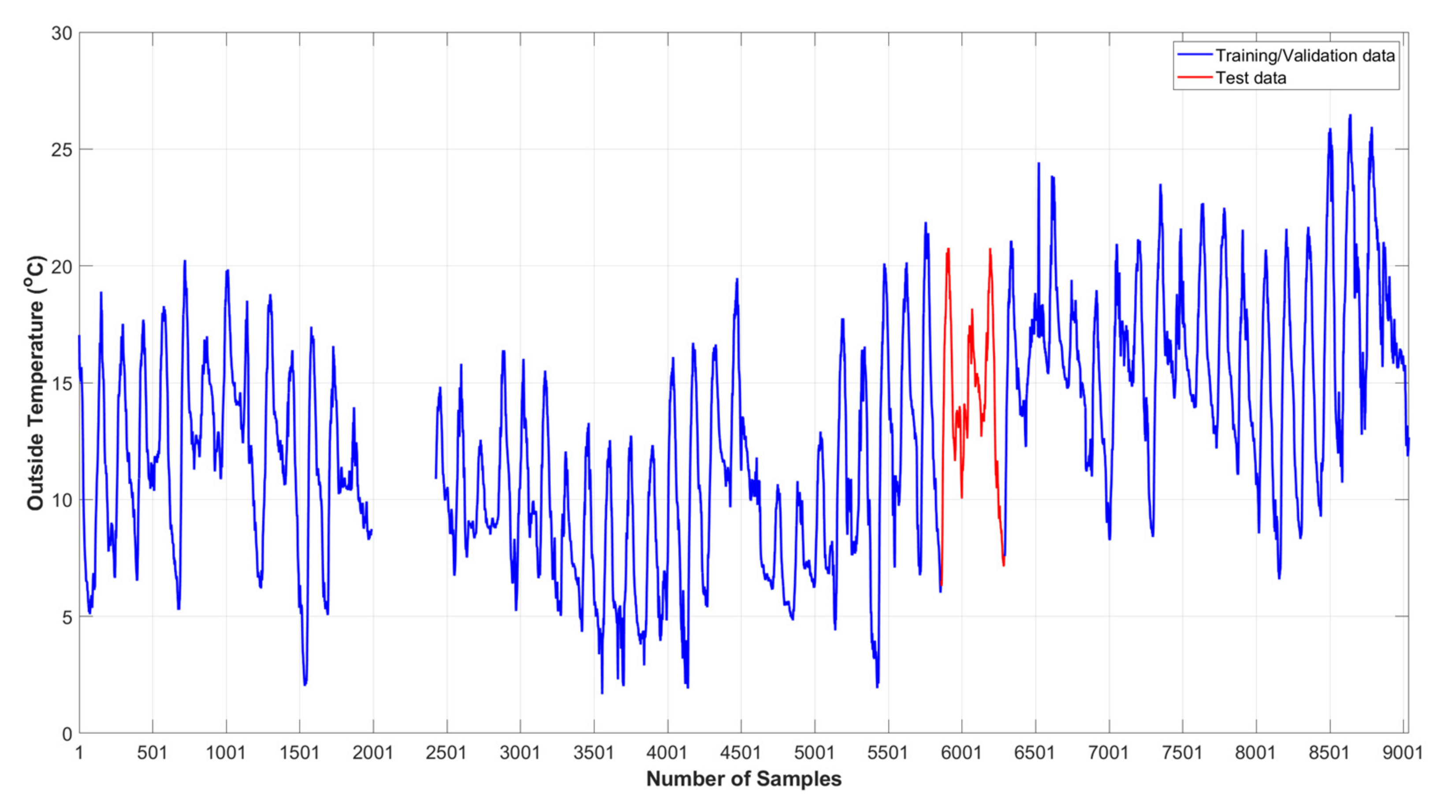
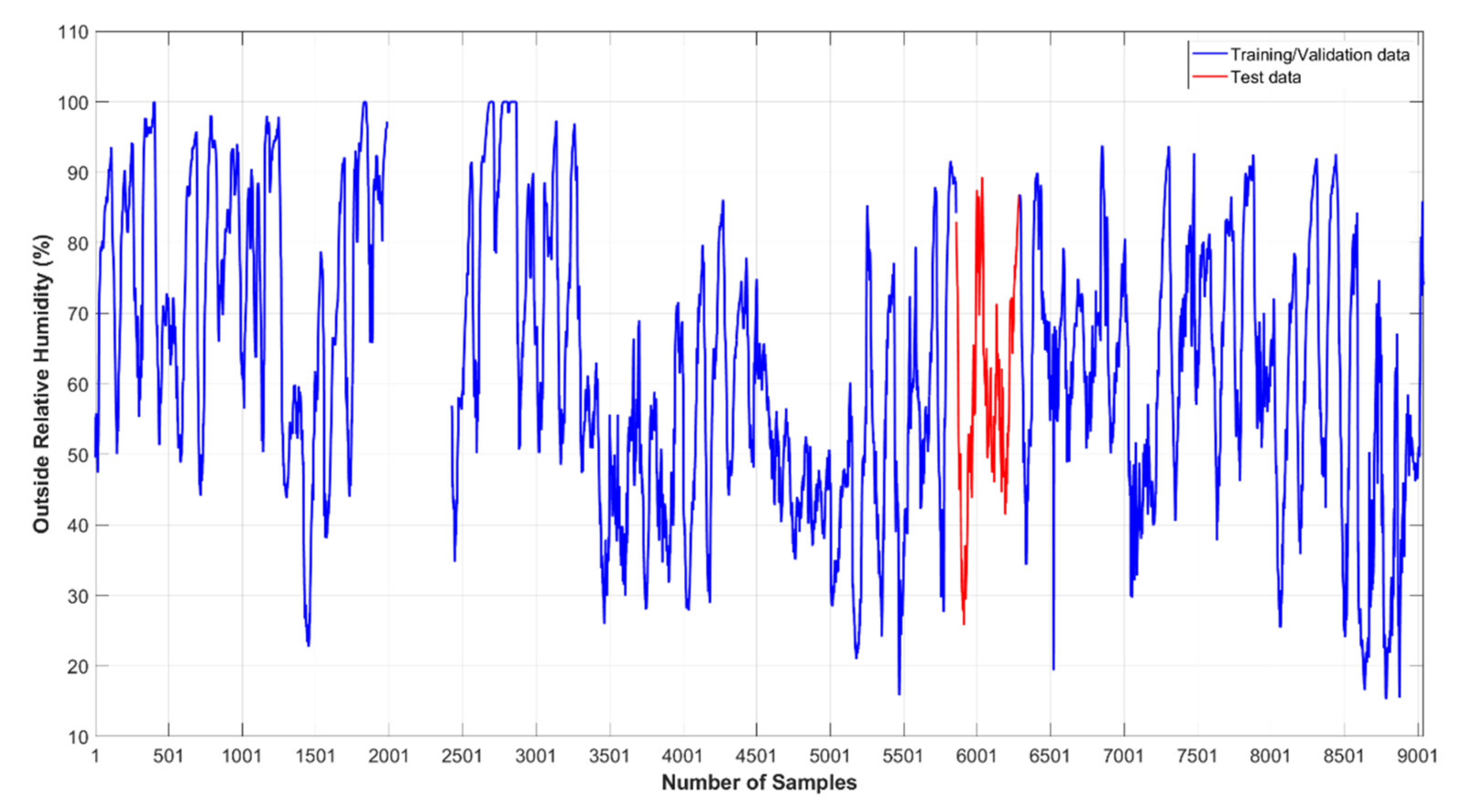
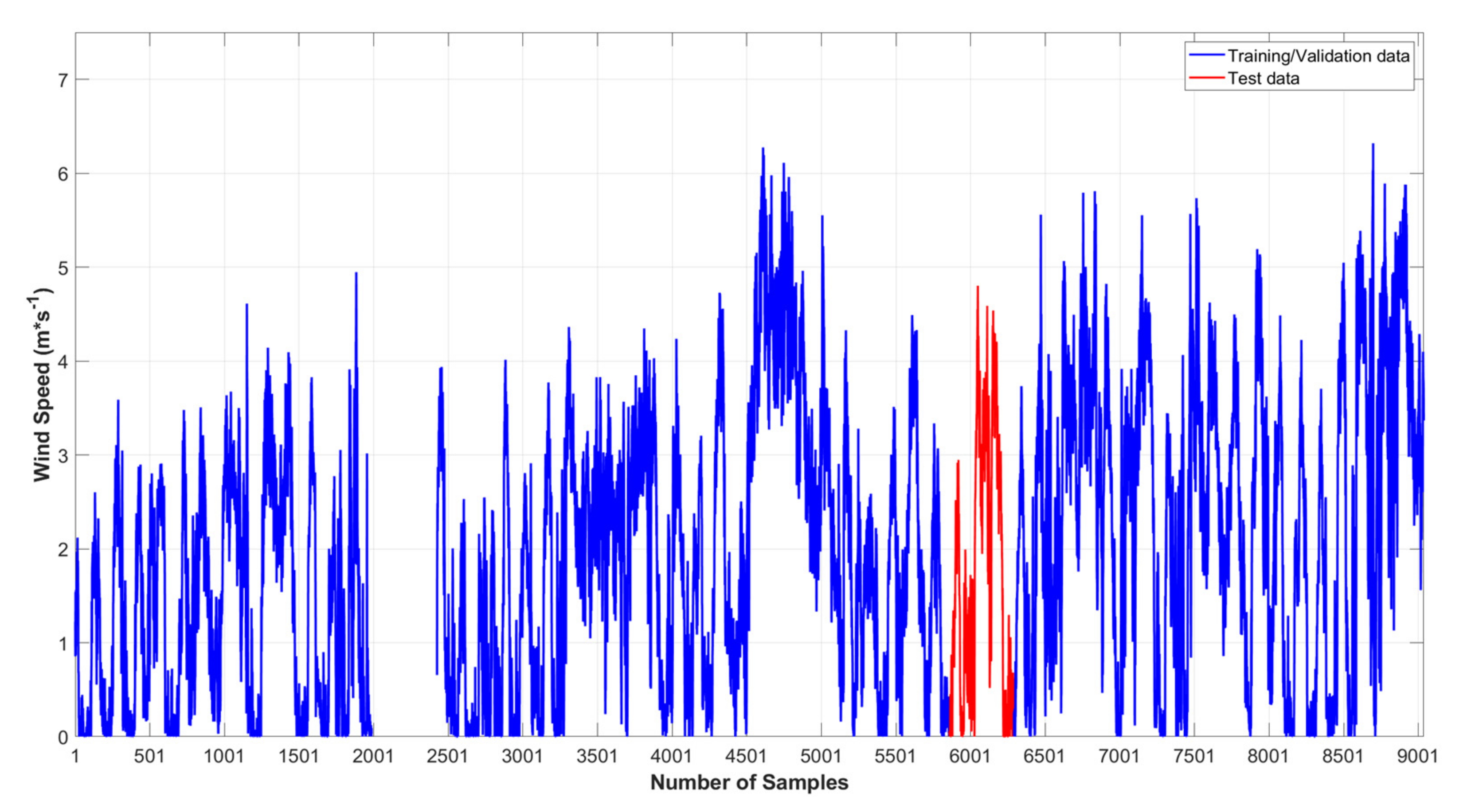
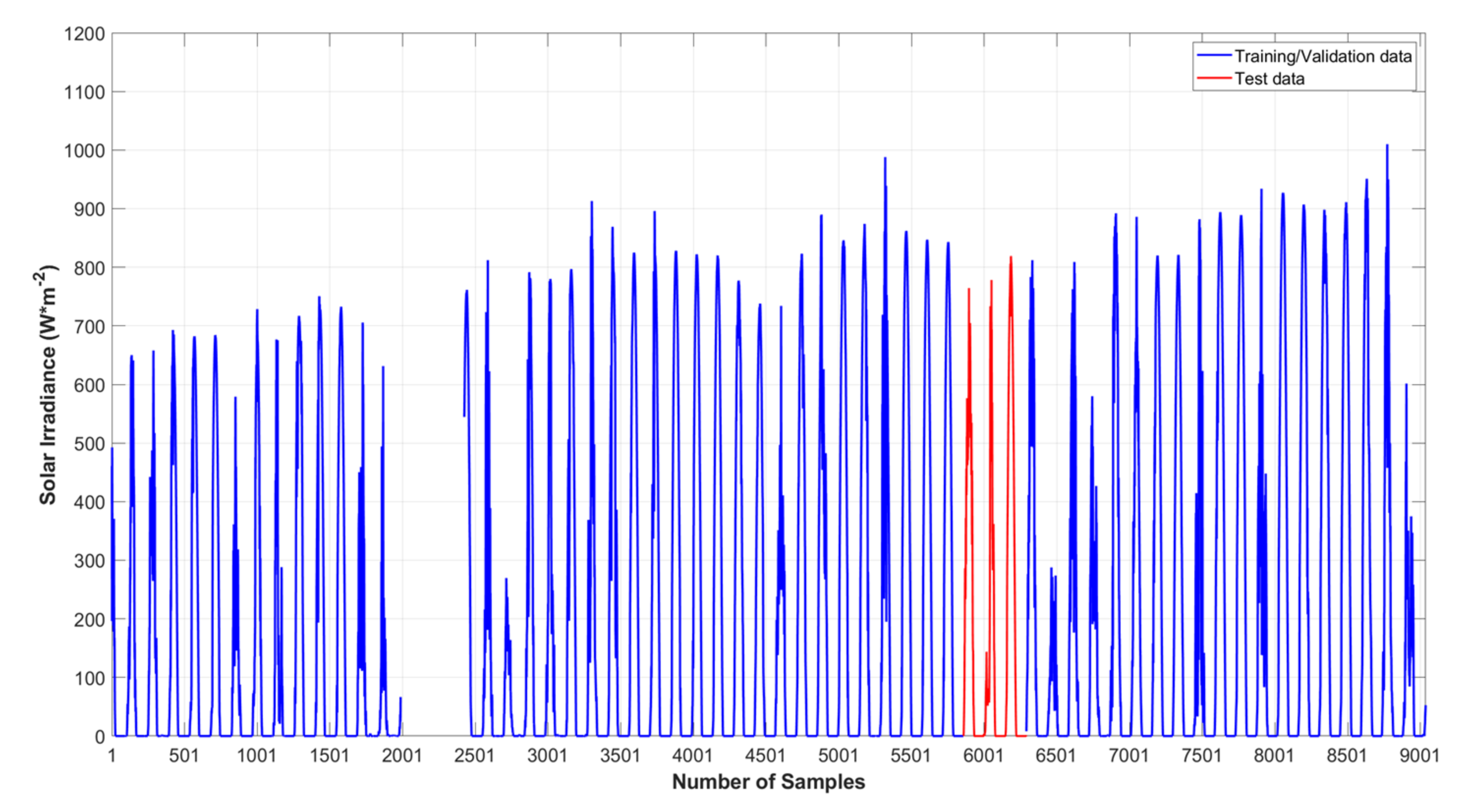
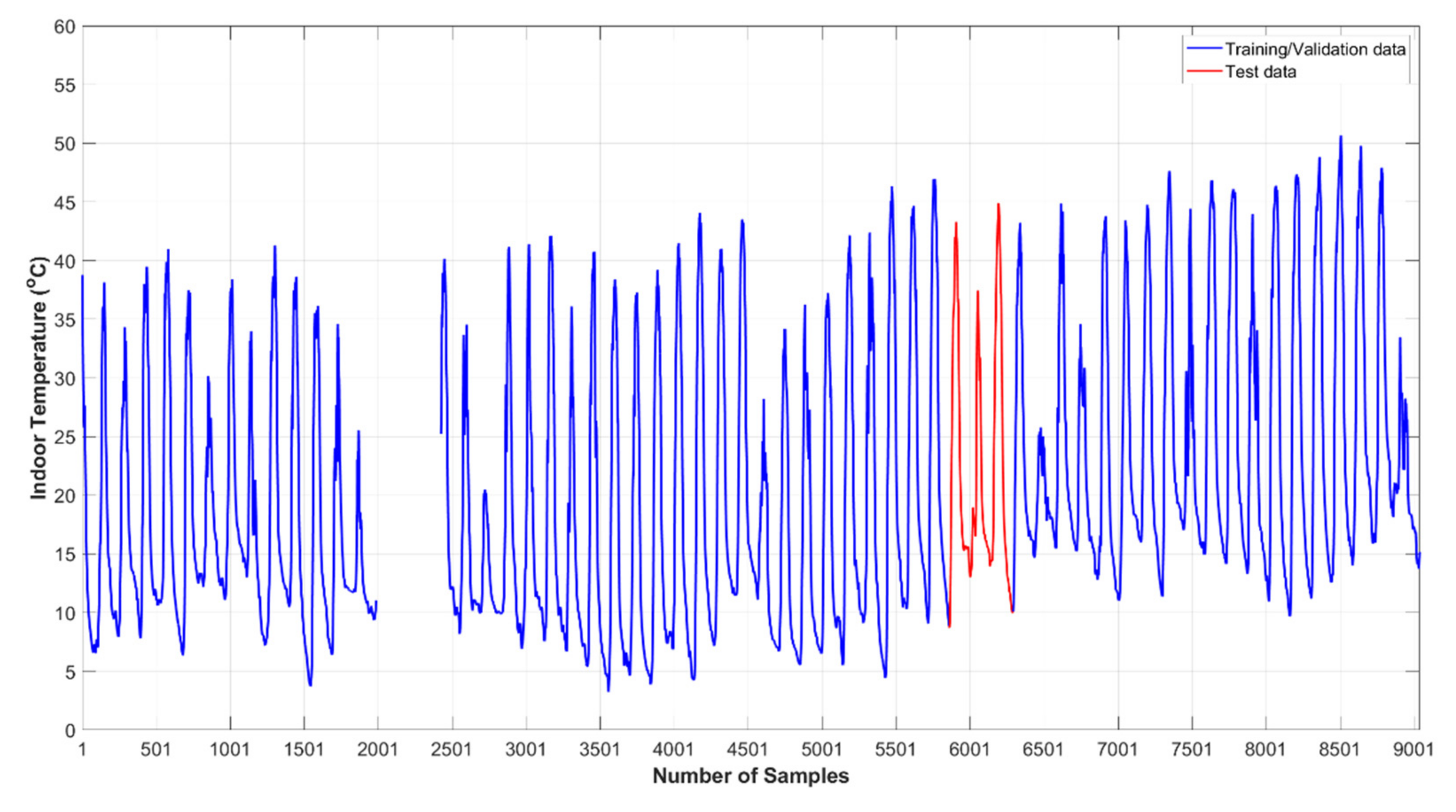
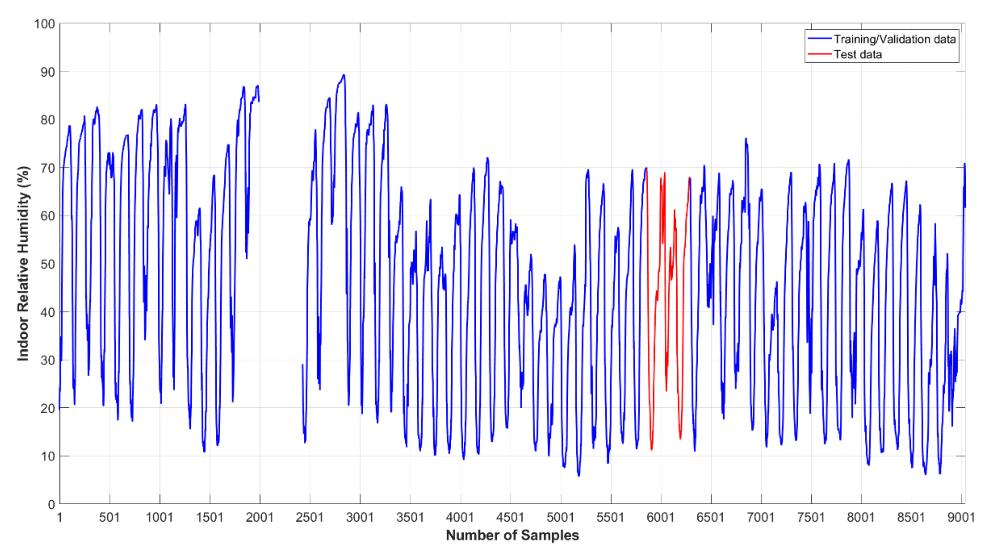
Figure 1, Figure 2, Figure 3, Figure 4, Figure 5 and Figure 6 show the time series for the above variables. For the specific period, the outside temperature ranges between 1.7 °C and 26.5 °C, outside relative humidity between 15.3% and 100%, wind speed between 0 and 6.3 m/s, and the maximum value for solar irradiance is 1010 W/m2. Inside the greenhouse, the temperature ranges between 3.2 °C and 50.7 °C, whereas relative humidity shows a minimum of 5.7% and a maximum of 89.3%.
As shown in the above figures, the input variables have neither the same units nor the same orders of magnitude. Thus, variables with higher values will contribute more to the output error, with the result that the algorithm gives more weight to them and less to variables with a smaller range of values [25]. For these reasons, it is necessary to normalize the variables in a range of 0 to 1 or −1 to 1, depending on the neural network activation function. In this study, the values of the input and output variables were normalized to a range between 0.01 and 0.99 according to Equation (3), where rmax and rmin are equal to 0.99 and 0.01, respectively. Min/max normalization was chosen because it is the fastest, easiest, and the most flexible normalization method, and with the addition of the parameters rmax and rmin, the normalization range can be easily changed depending on the needs of each activation function, setting the corresponding maximum and minimum limit of the range on them.
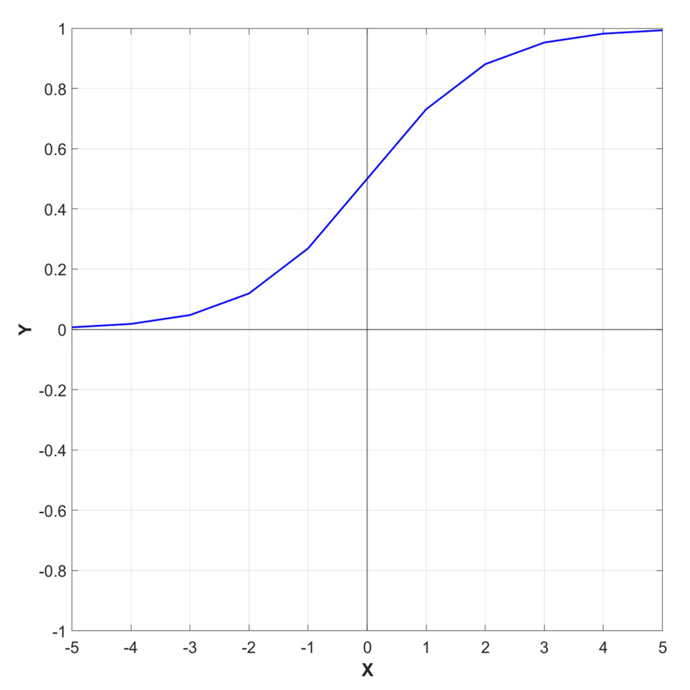
In Equation (3), Zi presents the normalized value of the Xi; Xmax and Xmin present the maximum and the minimum value of the variable X, respectively; and the parameters rmax and rmin obtain the values of the desired normalization range limits. This range was chosen due to the use of the logistic sigmoid activation function in the hidden layer of the neural network. The logistic sigmoid activation function is characterized by Equation (4) and receives values in a range of 0 to 1, as shown in Figure 7; however, it was chosen to use narrower boundaries due to the existence of possible discontinuities at the range limits. At the end of the process, the values were denormalized to complete the comparison between predictions and observations.
Then, after completing the preprocessing of the data, the dataset was divided into two different subsets. The first one, consisting of 59 days and a total number of 8161 samples, was randomly divided into two subsets with 80% of the samples used for training and the remaining 20% for the validation of the model. The remaining 3 days (433 samples) were used to test the model and to examine the model’s ability to generalize the results The 59-day time series (training/validation data) is represented in Figure 1, Figure 2, Figure 3, Figure 4, Figure 5 and Figure 6 by a blue line, while the 3-day time series (test data) from 27 March 2022 6:20 to 30 March 2022 6:20 is represented by a red line.
To check the results and the performance of the model the mean absolute error (MAE), the root mean square error (RMSE), and the coefficient of determination (R2) (Equations (4)–(6)), as well as the maximum error were calculated. The maximum error is a very important value for a decision support system, which will activate the various system management devices based on the results of the model.
2.3. Neural Network Model
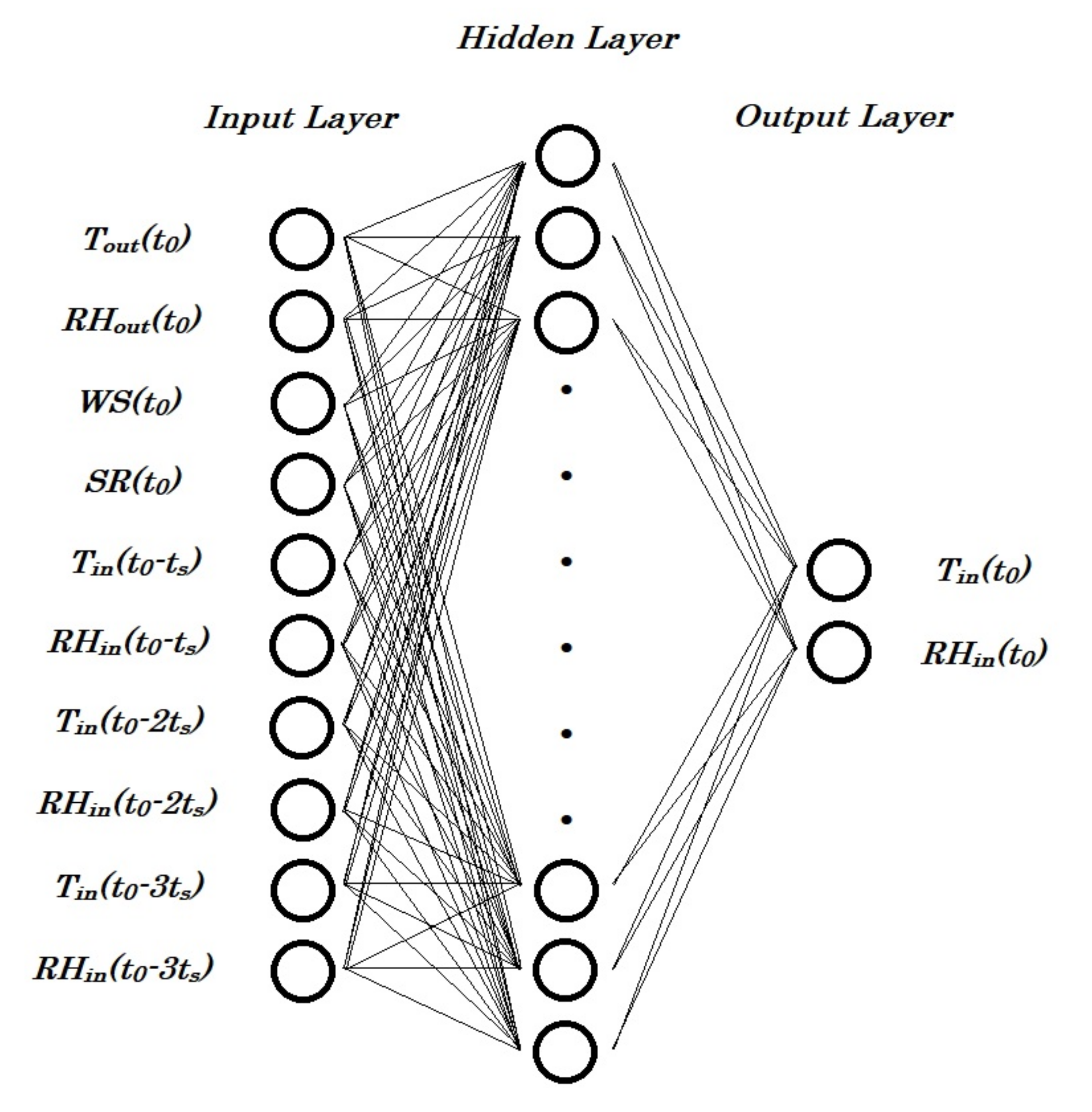
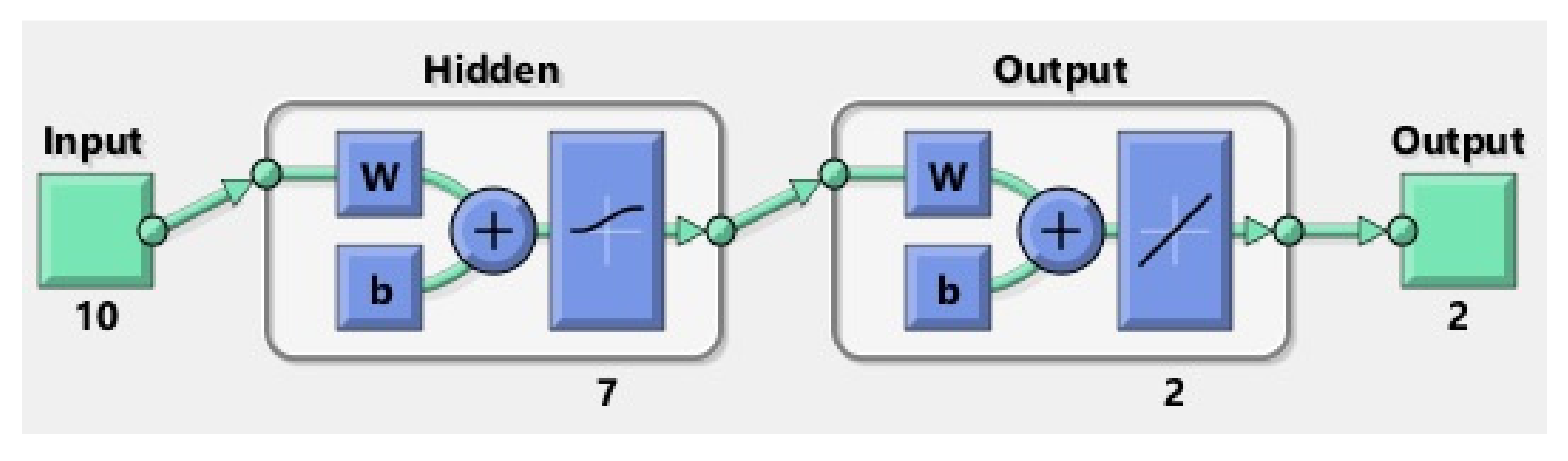
In this study, a multilayer perceptron (MLP) neural network was designed with three different layers, the input, the hidden, and the output layer. The input layer consists of 10 nodes, one for each independent variable, whereas the output layer consists of 2 nodes, one for the inside temperature and one for the relative humidity at time t0. As for the intermediate layers, the addition of a single hidden layer was chosen because according to Kolmogorov’s theorem, in an MLP neural network one hidden layer with a suitable number of nodes can give reliable results for any process [2,26].
The trial-and-error method to find the best neural network architecture, the best training algorithm, and the activation functions, was used. For the best architecture, the number of nodes within the hidden layer varied from time to time. The training algorithms tested were three of the most well-known algorithms, the Levenberg–Marquardt backpropagation algorithm, the Bayesian regularization backpropagation, and the BFGS quasi-Newton backpropagation; and four different activation functions for the hidden layer were also tested: the logistic sigmoid, the hyperbolic tangent sigmoid, the radial basis, and the positive linear. Table 2 presents the corresponding commands in the MATLAB programming language for both the above training algorithms and the activation functions.
Through the results, the Levenberg–Marquardt backpropagation algorithm was used as a training algorithm, an algorithm based on the Newton method. The LMBP training algorithm is a very reliable and fast solution for MLP neural networks and the optimization of function’s error consisting of a sum of squares of nonlinear processes [27,28]. Logistic sigmoid and linear were used as the activation functions for the hidden and output layers, respectively. Finally, mean square error (MSE) was used as a perform function. A diagram of the generated model is shown in Figure 8.
The model was developed and run with Matrix Laboratory (MATLAB).
3. Results and Discussion
In the present study, an MLP neural network was used for the prediction of the temperature and relative humidity inside the greenhouse. To find the best architecture, and more specifically the number of nodes in the hidden layer, the model was trained and tested for the corresponding periods mentioned in Section 2. After performing the procedure for a different number of nodes each time (from 1 to 20) and based on the statistical indices MAE, RMSE, R2, and the maximum error, it was found that the best structure of the neural network is 10-7-2, which gave the most reliable results for the testing period. The model structure extracted from MATLAB is presented in Figure 9, whereas the values of the aforementioned indices are presented in Table 3, both for temperature and relative humidity. According to the specific structure of the neural network, the following graphs of comparison were made between the observed and predicted values of the two variables.
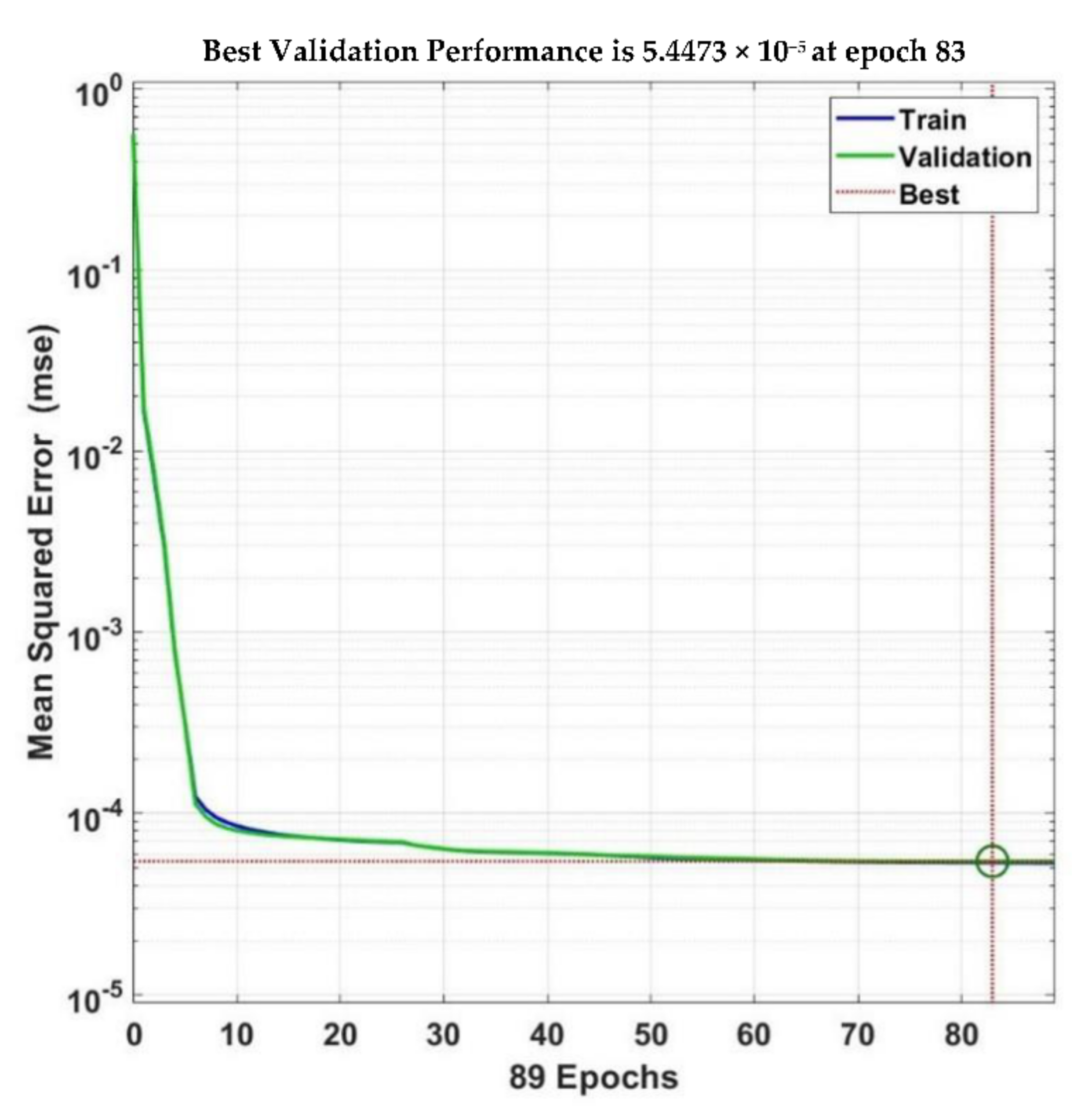
The model training process was completed after 89 epochs (Figure 10), where the validation mean square error (MSE) increased 6 times in a row. The number of epochs was selected to be 83 where the validation error presented its minimum value, which was equal to approximately 5.447 × 10⁻⁵. This value was obtained through the normalized input and output variables and presents the best performance of the model.
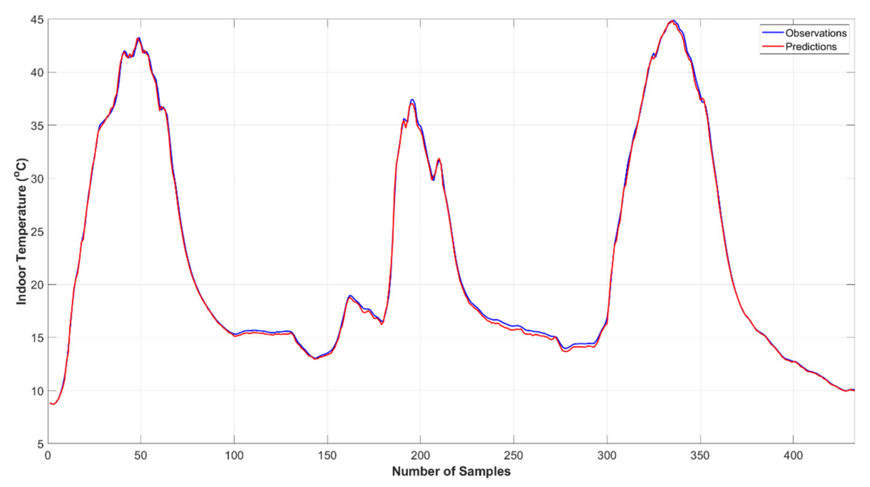
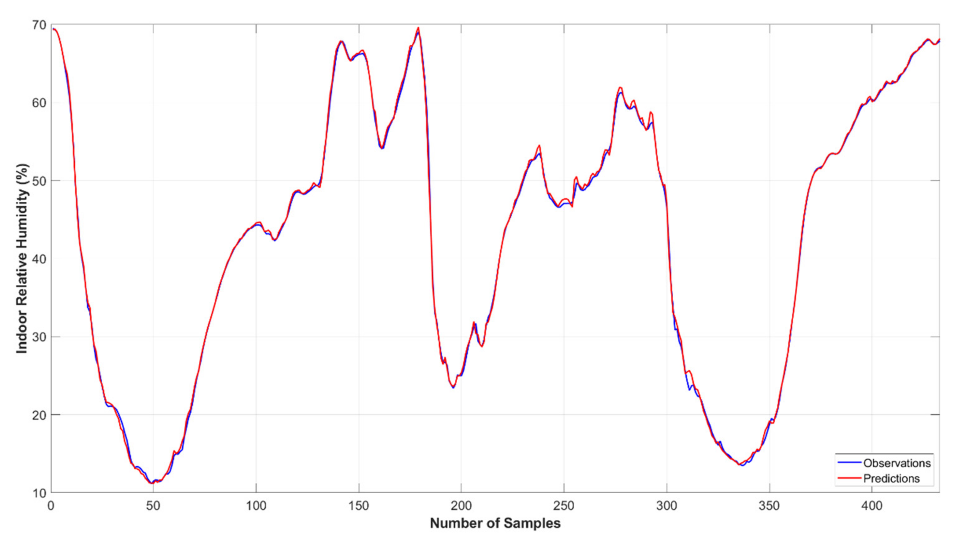
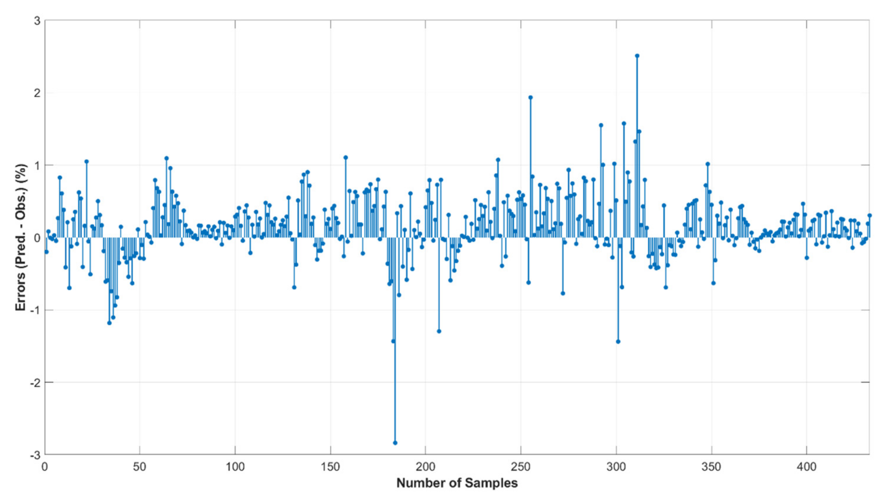
Regarding the greenhouse temperature and based on the values of the MAE and RMSE, which were calculated at 0.218 K and 0.271 K, the ability of the model to predict the temperature to a fairly satisfactory degree is established. At the same time, the values of MAE and RMSE differ slightly from each other, indicating the absence of large errors produced by the model. The relative humidity is on the same wavelength, with the values of MAE and RMSE being very small and equal to 0.339% and 0.48%, respectively. The coefficients of determination are the same for both parameters and equal to 0.999, which indicates the very good performance of the model. Finally, the maximum errors are equal to 0.877 K and 2.838% for temperature and relative humidity, respectively.
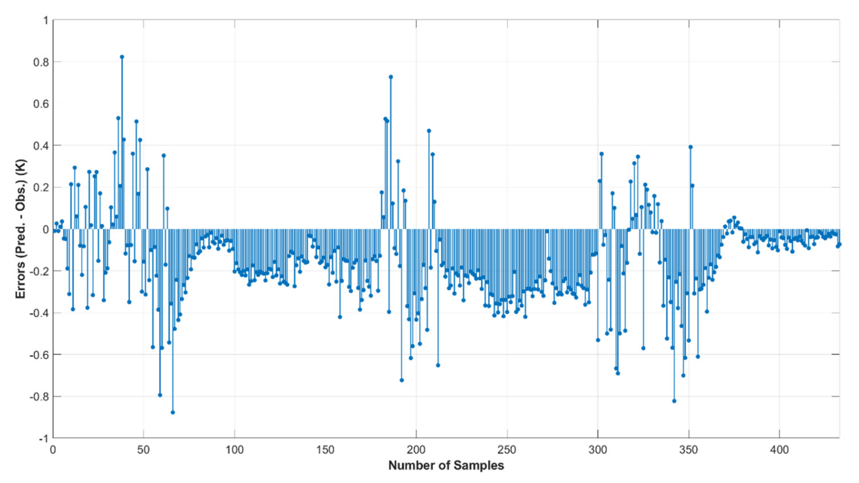
In Figure 11 and Figure 12, the time series of the predicted and observed temperature values for the 3 days used for testing the model are presented as well as the errors between the respective values. As shown in Figure 11, the model has predicted temperature to a large extent, and the largest errors occur during the daytime hours when the temperature presents high values but also abrupt changes (Figure 12). These errors have the potential to be reduced by adding more samples before training the model. In Figure 13 and in the case of relative humidity, great predictability is presented again, with the two curves being almost identical. However, according to Figure 14 and unlike the temperature case, errors do not seem to follow a fixed pattern.
In this study, to derive the optimal values of the model parameters, three different algorithms were initially used, the Levenberg–Marquardt backpropagation algorithm, the Bayesian regularization backpropagation algorithm, and the BFGS quasi-Newton backpropagation algorithm. The first of these three algorithms (methods) proved to be the best. In addition to the above, there are several different optimization techniques that could be used, such as different training algorithms (e.g., scaled conjugate gradient, conjugate gradient with Powell/Beale restarts, etc.). Relevant research comparing a large number of algorithms has already been conducted by Taki, et al. [24], with LMBP giving the best results.
Three different types of error descriptions were used to evaluate the results and compare the predicted and observed values for the two parameters under study (indoor temperature and relative humidity). Thus, the comparison of the results with a wide range of literature studies was achieved, as in each study a different formula was used to evaluate the error. The values calculated for the MAE and RMSE were found to be quite small, which gives the created model special weight. At the same time, after extensive research of the literature, the coefficients of determination, R2, for both temperature and relative humidity, proved to be very good, presenting values very close to 1. Finally, the maximum error is not a widespread data comparison value; however, for the needs of this work, it was a very useful parameter, with its value being quite small [29].
4. Conclusions
Modeling the greenhouse microclimate has proven to be a very difficult process due to the fact that a greenhouse is a dynamic system that is directly dependent on external environmental conditions, whereas the interactions between the parameters that constitute its internal conditions seem to be both strong and complex. Although physical models have been developed to estimate parameters such as indoor temperature and relative humidity, their complexity does not make them a useful tool, especially for decision support systems (DSS), which require models that in addition to high accuracy, can manage huge amounts of data with as little computing power as possible. The above requirements are largely met by modeling greenhouse conditions using artificial neural networks (ANNs), for which knowledge of physical processes is not necessary, providing a quick and easy way to assess the desired parameters through system identification processes.
The purpose of this study was to create a multilayer perceptron artificial neural network model to estimate indoor temperature and relative humidity, taking as input variables the outside temperature and relative humidity, the wind speed, the solar irradiance, and the indoor temperature and relative humidity with a time delay of three timesteps. Model predictions can be used as a basis for a DSS. The main goal was for the predictions’ maximum errors to be as small as possible, as this value plays a key role in a DSS. Even an incorrect prediction of the model is likely to either delay the operation of an actuator (e.g., heating or cooling system) or not even put it into operation, with crop destruction being a very likely possibility. At the same time, a clear assessment of the indoor environmental parameters will allow the actuators to be switched on only when really needed while keeping the energy consumption low.
Before the implementation of the model, the data were preprocessed, removing the missing values, and normalized into a range from 0.01 to 0.99 in order to avoid the weighted contribution due to the input variables’ different orders of magnitude. For the training and validation of the model, 59 days of data were used, which were randomly divided into two subsets, with 80% referring to the training process and 20% to the validation process. The three remaining days were used to test the model. The structure of the model consists of three different layers, the input, the hidden, and the output layer. The Levenberg–Marquardt backpropagation algorithm was selected through the trial-and-error method including two different algorithms, the Bayesian regularization backpropagation and the BFGS quasi-Newton backpropagation. logistic sigmoid and Llinear were used as the activation functions for the hidden layer and the output layer, respectively. The logistic sigmoid was chosen between the logistic sigmoid, the hyperbolic tangent sigmoid, the radial basis, and the positive linear. The model was implemented for a different number of nodes in the hidden layer (1 to 20), with the best results for the testing period being obtained for the 10-7-2 structure. The maximum error was equal to 0.877 K and 2.838% for temperature and relative humidity, respectively, and the MAE, RMSE, and R2 were calculated to equal 0.218 K, 0.271 K, and 0.999 for temperature, and to 0.339%, 0.481%, and 0.999 for relative humidity. The above values, both for the maximum error and for the rest of the statistics, prove that the specific model can satisfactorily meet the requirements of a decision support system.
The above-proposed model can respond to a DSS, making it a very important tool. However, the existence of a crop inside the greenhouse could create problems in extracting reliable results from the model. Introducing biological processes, such as evapotranspiration, relative humidity, and consequently temperature, would add one more factor to influence them besides the conditions of the external environment. At the same time, as found in the results, the largest errors of the model occur at times when both the temperature and the relative humidity show abrupt changes. Therefore, the ability of the model to predict the above parameters should be studied in case the presence of actuators (e.g., heating systems, dynamic ventilation) causes relatively abrupt changes in the microclimate of the greenhouse. Finally, adding data describing extreme conditions, such as a summer heatwave or a very cold winter day, will be able to train the model in extreme cases that could cause significant crop problems. Future work could include studying the ability of the model to predict the temperature and the relative humidity under the influence of a crop on the internal greenhouse conditions, the addition of parameters concerning the actuators of the greenhouse but also the addition of more data to the model and train it in further cases, and gaining the ability to respond to extreme conditions and rapid dynamic changes.
Author Contributions
Conceptualization, T.P. and A.K.; methodology, A.K.; software, T.P. and V.T.; validation, A.K. and A.A.A.; formal analysis, T.P., A.K., V.T. and A.A.A.; investigation, T.P.; resources, A.K.; data curation, T.P.; writing—original draft preparation, T.P.; writing—review and editing, T.P., A.K., V.T. and A.A.A.; visualization, T.P.; supervision, A.K.; project administration, A.K.; funding acquisition, A.K. All authors have read and agreed to the published version of the manuscript.
Funding
This research has been co-financed by the European Union and Greek national funds through the Operational Program “Crete 2014–2020”, under the call “Business partnerships with Research and Dissemination Organizations, in RIS3Crete sectors” (project “Implementation of intelligent and sustainable model greenhouse unit with application of innovative information and control technologies—SmartGreen”, code: KPHP1-0028613/MIS 5063262).
Institutional Review Board Statement
Not applicable.
Informed Consent Statement
Not applicable.
Data Availability Statement
The computer codes created and implemented in MATLAB for the needs of this research, as well as the data used, have been deposited on the public repository GitHub. Access can be obtained via the following link available online: https://github.com/thodorisptrks/Greenhouse_Dep_of_Agric_UPAT (accessed on 26 May 2022).
Acknowledgments
The present work was financially supported by the «Andreas Mentzelopoulos Foundation».
Conflicts of Interest
The authors declare no conflict of interest.
References
- Aslan, M.F.; Durdu, A.; Sabanci, K.; Ropelewska, E.; Gültekin, S.S. A Comprehensive Survey of the Recent Studies with UAV for Precision Agriculture in Open Fields and Greenhouses. Appl. Sci. 2022, 12, 1047. [Google Scholar] [CrossRef]
- Singh, V.K.; Tiwari, K.N. Prediction of greenhouse micro-climate using artificial neural network. Appl. Ecol. Environ. Res. 2017, 15, 767–778. [Google Scholar] [CrossRef]
- Shamshiri, R.R.; Jones, J.W.; Thorp, K.R.; Ahmad, D.; Man, H.C.; Taheri, S. Review of optimum temperature, humidity, and vapour pressure deficit for microclimate evaluation and control in greenhouse cultivation of tomato: A review. Int. Agrophys. 2018, 32, 287–302. [Google Scholar] [CrossRef]
- Rabbi, B.; Chen, Z.-H.; Sethuvenkatraman, S. Protected Cropping in Warm Climates: A Review of Humidity Control and Cooling Methods. Energies 2019, 12, 2737. [Google Scholar] [CrossRef] [Green Version]
- Soussi, M.; Chaibi, M.T.; Buchholz, M.; Saghrouni, Z. Comprehensive Review on Climate Control and Cooling Systems in Greenhouses under Hot and Arid Conditions. Agronomy 2022, 12, 626. [Google Scholar] [CrossRef]
- Shen, Y.; Wei, R.; Xu, L. Energy Consumption Prediction of a Greenhouse and Optimization of Daily Average Temperature. Energies 2018, 11, 65. [Google Scholar] [CrossRef] [Green Version]
- Savvas, D.; Ropokis, A.; Ntatsi, G.; Kittas, C. Current situation of greenhouse vegetable production in Greece. In Proceedings of the VI Balkan Symposium on Vegetables and Potatoes, Zagreb, Croatia, 29 September 2014. [Google Scholar]
- Kavga, A.; Thomopoulos, V.; Barouchas, P.; Stefanakis, N.; Liopa-Tsakalidi, A. Research on Innovative Training on Smart Greenhouse Technologies for Economic and Environmental Sustainability. Sustainability 2021, 13, 10536. [Google Scholar] [CrossRef]
- Stull, R. An Introduction to Boundary Layer Meteorology, 1st ed.; Kluwer Academic Publishers: Dordrecht, The Netherlands, 1988; pp. 2–3. [Google Scholar]
- Maher, A.; Kamel, E.; Enrico, F.; Abdelkader, M. An intelligent system for the climate control and energy savings in agricultural greenhouses. Energy Effic. 2016, 9, 1241–1255. [Google Scholar] [CrossRef]
- Francik, S.; Kurpaska, S. The Use of Artificial Neural Networks for Forecasting of Air Temperature inside a Heated Foil Tunnel. Sensors 2020, 20, 652. [Google Scholar] [CrossRef] [Green Version]
- Cañadas, J.; Sánchez-Molina, J.A.; Rodríguez, F.; del Águila, I.M. Improving automatic climate control with decision support techniques to minimize disease effects in greenhouse tomatoes. Inf. Process. Agric. 2017, 4, 50–63. [Google Scholar] [CrossRef]
- Lopez-Cruz, I.L.; Fitz-Rodríguez, E.; Raquel, S.; Rojano-Aguilar, A.; Kacira, M. Development and analysis of dynamical mathematical models of greenhouse climate: A review. Eur. J. Hortic. Sci. 2018, 83, 269–279. [Google Scholar] [CrossRef]
- Choab, N.; Allouhi, A.; El Maakoul, A.; Kousksou, T.; Saadeddine, S.; Jamil, A. Review on greenhouse microclimate and application: Design parameters, thermal modeling and simulation, climate controlling technologies. Sol. Energy 2019, 191, 109–137. [Google Scholar] [CrossRef]
- Su, Y.; Xu, L. Towards discrete time model for greenhouse climate control. Eng. Agric. Environ. Food 2017, 10, 157–170. [Google Scholar] [CrossRef]
- Zhang, P. Industrial control system simulation routines. In Advanced Industrial Control Technology, 1st ed.; Elsevier Inc.: Amsterdam, The Netherlands, 2010; pp. 781–810. [Google Scholar] [CrossRef]
- Esteves, M.S.; Perdicoúlis, T.P.A.; dos Santos, P.L. System Identification Methods for Identification of State Models. In Proceedings of the 11th Portuguese Conference on Automatic Control (CONTROLO’2014), Porto, Portugal, 21–23 July 2014; Volume 321. [Google Scholar] [CrossRef]
- Escamilla-García, A.; Soto-Zarazúa, G.M.; Toledano-Ayala, M.; Rivas-Araiza, E.; Gastélum-Barrios, A. Applications of Artificial Neural Networks in Greenhouse Technology and Overview for Smart Agriculture Development. Appl. Sci. 2020, 10, 3835. [Google Scholar] [CrossRef]
- Calderón, A.; González, I. Neural Networks-based models for greenhouse climate control. In Proceedings of the XXXIX Jornadas de Automática, Badajoz, Spain, 5–7 September 2018. [Google Scholar]
- Castañeda-Miranda, A.; Castaño, V. Smart frost control in greenhouses by neural networks models. Comput. Electron. Agric. 2017, 137, 102–114. [Google Scholar] [CrossRef]
- Choi, H.; Moon, T.; Jung, D.H.; Son, J.E. Prediction of Air Temperature and Relative Humidity in Greenhouse via a Mutlilayer Perceptron Using Environmental Factors. Prot. Hortic. Plant Fact. 2019, 28, 95–103. [Google Scholar] [CrossRef]
- Hongkang, W.; Li, L.; Yong, W.; Fanjia, M.; Haihua, W.; Sigrimis, N.A. Recurrent Neural Network Model for Prediction of Microclimate in Solar Greenhouse. In Proceedings of the 6th IFAC Conference on Bio-Robotics (BIOROBOTICS 2018), Beijing, China, 13–15 July 2018. [Google Scholar] [CrossRef]
- Salah, L.B.; Fourati, F. A greenhouse modeling and control using deep neural networks. Appl. Artif. Intell. 2021, 35, 1905–1929. [Google Scholar] [CrossRef]
- Taki, M.; Mehdizadeh, S.A.; Rohani, A.; Rahnama, M.; Rahmati-Joneidabad, M. Applied machine learning in greenhouse simulation; new application and analysis. Inf. Process. Agric. 2018, 5, 253–268. [Google Scholar] [CrossRef]
- Bhanja, S.; Das, A. Impact of Data Normalization on Deep Neural Network for Time Series Forecasting. arXiv 2018, arXiv:1812.05519. [Google Scholar]
- Schmidt-Hieber, J. The Kolmogorov-Arnold representation theorem revisited. Neural Netw. 2021, 137, 119–126. [Google Scholar] [CrossRef]
- Yang, B.; Chen, Y.; Guo, Z.; Wang, J.; Zeng, C.; Li, D.; Shu, H.; Shan, J.; Fu, T.; Zang, X. Levenberg-Marquardt backpropagation algorithm for parameter identification of solid oxide fuel cells. Int. J. Energy Res. 2021, 45, 17903–17923. [Google Scholar] [CrossRef]
- Lv, C.; Xing, Y.; Zhang, J.; Na, X.; Li, Y.; Liu, T.; Cao, D.; Wang, F.Y. Levenberg–Marquardt Backpropagation Training of Multilayer Neural Networks for State Estimation of a Safety-Critical Cyber-Physical System. IEEE Trans. Ind. Inform. 2018, 14, 3436–3446. [Google Scholar] [CrossRef] [Green Version]
- Aslan, M.F.; Durdu, A.; Sabanci, K. Human action recognition with bag of visual words using different machine learning methods and hyperparameter optimization. Neural Comput. Appl. 2020, 32, 8585–8597. [Google Scholar] [CrossRef]
Figure 1.
Outside temperature training/validation and test data.

Figure 2.
Outside relative humidity training/validation and test data.

Figure 3.
Wind speed training/validation and test data.

Figure 4.
Solar irradiance training/validation and test data.

Figure 5.
Indoor temperature training/validation and test data.

Figure 6.
Indoor relative humidity training/validation and test data.

Figure 7.
Graphic illustration of logistic sigmoid activation function.

Figure 8.
Scheme of the neural network structure.

Figure 9.
ANN model structure in MATLAB.

Figure 10.
Convergence of mean square error with epochs throughout training and validation process.

Figure 11.
Comparison between indoor temperature predictions and observations for the testing period and 10-7-2 NN structure.
Figure 11.
Comparison between indoor temperature predictions and observations for the testing period and 10-7-2 NN structure.

Figure 12.
Errors between indoor temperature predictions and observations for the testing period and 10-7-2 NN structure.
Figure 12.
Errors between indoor temperature predictions and observations for the testing period and 10-7-2 NN structure.

Figure 13.
Comparison between indoor relative humidity predictions and observations for the testing period and 10-7-2 NN structure.
Figure 13.
Comparison between indoor relative humidity predictions and observations for the testing period and 10-7-2 NN structure.

Figure 14.
Errors between indoor relative humidity and observations for the testing period and 10-7-2 NN structure.
Figure 14.
Errors between indoor relative humidity and observations for the testing period and 10-7-2 NN structure.


Table 1.
Recorded parameters, sensors used to record them, and sensor manufacturers.
| Recorded Parameter | Sensor | Manufacturer |
|---|---|---|
| Automatic Weather Station | ||
| Datalogger | CR1000 | Campbell Scientific |
| Temperature (Tout) | MP101A-T7-WAW at 3 m | Rotronic |
| Relative Humidity (RHout) | MP101A-T7-WAW at 3 m | Rotronic |
| Wind Speed (WS) | A100K at 6 m | Scienter |
| Solar Radiation (SRout) | CMP3 at 5 m | Kipp & Zonen |
| Rainfall (R) | 52203 | Campbell Scientific |
| Sky Temperature (Tsky) | CGR3 at 5 m | Kipp & Zonen |
| IR Radiation (IRrad) | CGR3 at 5 m | Kipp & Zonen |
| Greenhouse | ||
| Temperature (Tin,1 & Tin,2) | MP101A-T7-WAW | Rotronic |
| Relative Humidity (RHin,1 & RHin,2) | MP101A-T7-WAW | Rotronic |
| Solar Radiation (SRin,1 & SRin,2) | CMP3 | Kipp & Zonen |
| Photosynthetically Active Radiation (PAR1 & PAR2) | ParLite | Kipp & Zonen |
Table 2.
MATLAB for the tested training algorithms and activation functions.
| Name | MATLAB Coding |
|---|---|
| Training Algorithm | |
| Levenberg–Marquardt backpropagation | “trainlm” |
| Bayesian Regularization backpropagation | “trainbr” |
| BFGS Quasi Newton backpropagation | “trainbfg” |
| Activation Function | |
| Logistic Sigmoid | “logsig” |
| Hyperbolic Tangent Sigmoid | “tansig” |
| Radial Basis | “radbas” |
| Positive Linear | “poslin” |
Table 3.
Statistical indicators of comparison between observed and predicted values of internal temperature and relative humidity.
Table 3.
Statistical indicators of comparison between observed and predicted values of internal temperature and relative humidity.
| Statistical Indicators | Temperature | Relative Humidity |
|---|---|---|
| MAE | 0.218 K | 0.339% |
| RMSE | 0.271 K | 0.481% |
| R2 | 0.999 | 0.999 |
| MAX ERROR | 0.877 K | 2.838% |
Publisher’s Note: MDPI stays neutral with regard to jurisdictional claims in published maps and institutional affiliations. |
© 2022 by the authors. Licensee MDPI, Basel, Switzerland. This article is an open access article distributed under the terms and conditions of the Creative Commons Attribution (CC BY) license (https://creativecommons.org/licenses/by/4.0/).
Share and Cite
MDPI and ACS Style
Petrakis, T.; Kavga, A.; Thomopoulos, V.; Argiriou, A.A. Neural Network Model for Greenhouse Microclimate Predictions. Agriculture 2022, 12, 780. https://0-doi-org.brum.beds.ac.uk/10.3390/agriculture12060780
AMA Style
Petrakis T, Kavga A, Thomopoulos V, Argiriou AA. Neural Network Model for Greenhouse Microclimate Predictions. Agriculture. 2022; 12(6):780. https://0-doi-org.brum.beds.ac.uk/10.3390/agriculture12060780
Chicago/Turabian StylePetrakis, Theodoros, Angeliki Kavga, Vasileios Thomopoulos, and Athanassios A. Argiriou. 2022. "Neural Network Model for Greenhouse Microclimate Predictions" Agriculture 12, no. 6: 780. https://0-doi-org.brum.beds.ac.uk/10.3390/agriculture12060780
Note that from the first issue of 2016, this journal uses article numbers instead of page numbers. See further details here.