
Tea Tree Pest Detection Algorithm Based on Improved Yolov7-Tiny


1
College of Mathematics and Computer Science, Zhejiang A&F University, Hangzhou 311300, China
2
Key Laboratory of Forestry Intelligent Monitoring and Information Technology of Zhejiang Province, Hangzhou 311300, China
3
China Key Laboratory of State Forestry and Grassland Administration on Forestry Sensing Technology and Intelligent Equipment, Hangzhou 311300, China
4
College of Optical, Mechanical and Electrical Engineering, Zhejiang A&F University, Lin′an, Hangzhou 311300, China
*
Author to whom correspondence should be addressed.
Agriculture 2023, 13(5), 1031; https://0-doi-org.brum.beds.ac.uk/10.3390/agriculture13051031
Submission received: 19 April 2023
/
Revised: 5 May 2023
/
Accepted: 6 May 2023
/
Published: 9 May 2023
(This article belongs to the Section Digital Agriculture)
Abstract
:Timely and accurate identification of tea tree pests is critical for effective tea tree pest control. We collected image data sets of eight common tea tree pests to accurately represent the true appearance of various aspects of tea tree pests. The dataset contains 782 images, each containing 1~5 different pest species randomly distributed. Based on this dataset, a tea garden pest detection and recognition model was designed using the Yolov7-tiny network target detection algorithm, which incorporates deformable convolution, the Biformer dynamic attention mechanism, a non-maximal suppression algorithm module, and a new implicit decoupling head. Ablation experiments were conducted to compare the performance of the models, and the new model achieved an average accuracy of 93.23%. To ensure the validity of the model, it was compared to seven common detection models, including Efficientdet, Faster Rcnn, Retinanet, DetNet, Yolov5s, YoloR, and Yolov6. Additionally, feature visualization of the images was performed. The results demonstrated that the Improved Yolov7-tiny model developed was able to better capture the characteristics of tea tree pests. The pest detection model proposed has promising application prospects and has the potential to reduce the time and economic cost of pest control in tea plantations.
1. Introduction
The leaves of the tea tree can be used to make tea, the seeds can be used to extract oil, and the wood of the tea tree is of fine quality and can be used for carving. As an economically and environmentally friendly crop, the tea tree has applications in various fields, such as agriculture, food and beverage, medical and health care, daily necessities, and ecological tourism [1,2]. Therefore, the tea tree is an important cash crop, and its variety directly affects the yield, quality, and economic benefits of tea production [3]. However, tea tree cultivation is susceptible to pests, with more than a dozen common pests known to affect tea tree plants, including small green leafhoppers, tea-winged stink bugs, green blind stink bugs, golden turtles, and others. In order to effectively prevent and control the occurrence of pests, ensure the quality of tea production, and improve overall tea yield, it is of great practical significance to study effective methods for tea tree pest control [4].
In the past, the judgment of tea tree pests often relied on the practical experience of farmers [5], but this method is labor-intensive and prone to misjudgment, resulting in higher costs. As a result, researchers have explored various technical methods for pest detection, including sound signal-based detection methods and near-infrared light-based detection methods [6,7]. However, these methods have limitations and may not yield satisfactory results in practical application scenarios.
With the advancement of computer vision and machine learning, these technologies are now widely utilized in agricultural production [8]. For instance, Larios et al., (2008) proposed a fast classification system for stonefly larvae that incorporated transport and imaging devices [9]. They designed a Principal Curvature-Based Region (PCBR) detector to represent these regions and integrated it with a classification algorithm to achieve 82% detection accuracy for four classes. Yaakob et al., (2012) successfully combined moment invariant techniques with neural networks to identify 20 classes of insects [10]. They utilized six invariant moment feature extraction algorithms and classified these features effectively using the ARTMAP neural network algorithm. Espinoza et al., (2016) proposed a method combining image processing and artificial neural networks to detect and identify white whitefly and thrip adults in a greenhouse environment [11]. They use the techniques of object detection, segmentation, morphology, and color attribute estimation to process the objects in the image, and finally use the feedforward multi-layer artificial neural network to realize recognition and classification. Pujari D et al., (2016) proposed a simplified feature set based method for plant disease image recognition and classification [12]. The results show that support vector machine classifier is more suitable for the recognition and classification of agronomic crop diseases. Thenmozhi et al., (2017) employed image processing techniques to preprocess images of sugarcane crop insects and applied the Sobel edge detection algorithm to segment the images for identification based on nine shape features [13]. They tested insects on round, oval, triangular, and rectangular sugarcane crops and demonstrated that they worked successfully in all cases to extract insect outlines. Ebrahima et al., (2017) applied an SVM algorithm to identify strawberry thrips in greenhouses [14]. The characteristic parameters of this experiment are divided into two categories. One is color characteristic parameters: hue, saturation, and brightness. The other is the regional characteristic parameter: the ratio of large diameter to small diameter of the target. Finally, the average error rate of this experiment is less than 2.25%. However, traditional methods of extracting image features tend to rely on manual design and may only be applicable in specific scenarios with limited generalization ability. This poses challenges in extending these features to practical applications and lacks guidance for pest detection research in large-scale categories in natural environments. Therefore, further in-depth research is needed for image-based pest detection techniques.
With the development of deep learning technology, particularly with the introduction of AlexNet by Krizhevsky in 2012 [15], deep learning techniques have rapidly advanced and are now widely used in various fields, including autonomous driving [16,17], fault detection [18,19], medical decision making [20,21], and agriculture [22,23]. In 2018, Shen et al. proposed a faster-RCNN-based pest detection method for grain silos [24], where the feature extraction structure of Faster-RCNN was replaced with the inception structure to identify and classify six common grain bin pests, achieving an average accuracy of 88% for grain bin pest detection. Li et al., (2019) proposed a coarse-to-fine convolutional neural network (CFN) to address the challenge of detecting aggregated small aphids [25], where the network first detected dense areas of pests and then detected small aphids in those dense areas, achieving an average precision (AP) value of 76.8% in detection. Tetila et al., (2020) used the SLIC superpixel algorithm to segment and identify soybean pest images [26] and evaluated five deep learning networks with different fine-tuning and migration strategies, comparing them with other machine learning methods. The detection method based on the ResNet-50 architecture achieved an accuracy of 93.82% on the soybean pest dataset. Chen et al., (2021). proposed a model that integrated an attention mechanism and a classification activation map in MobileNet-V2 to improve the network’s learning ability on pest images in complex contexts [27]. Their proposed model achieved an average accuracy of 99.14% on open datasets and 92.79% under special context conditions.
Convolutional neural networks (CNNs) can automatically learn image features and perform image feature recognition through a series of convolutional filters [28,29], which have stronger feature extraction ability, accuracy, and generalization compared to traditional image recognition methods. However, there is still a wide range of shortcomings in most of the aforementioned studies. From the application perspective, most of the studies struggle with distinguishing pests, and there are few models available to accurately identify different species within the same genus. Additionally, the majority of studies focus on pests in grain bins, fields, fruits, and vegetables, with limited research on tea tree pests. There is also a lack of effective models for achieving accurate results in detecting heavily obscured targets. At the algorithm level, existing models may encounter problems such as incorrect detection, missed detection, and multiple detections during the pest detection process. The complex background of tea trees in real environments, along with the subtle differences between pests of different species within the same genus, make accurate detection challenging for deep learning models. Furthermore, a large amount of image data is required to train deep learning models for pest detection, but currently, models with high computational and parametric requirements may not be widely accessible. Models with limited computational power may also have poor detection performance.
In order to solve the above problems, we focus on improving the capability of the feature extraction network, enhancing the performance of the feature fusion network, and propose a new implicit decoupling head at the output end to make it pay more attention to the target to be detected and improve the detection capability of the prediction module. Improved Yolov7-tiny model improves the detection ability and efficiency of tea plant pests.
2. Materials and Methods
2.1. Methods
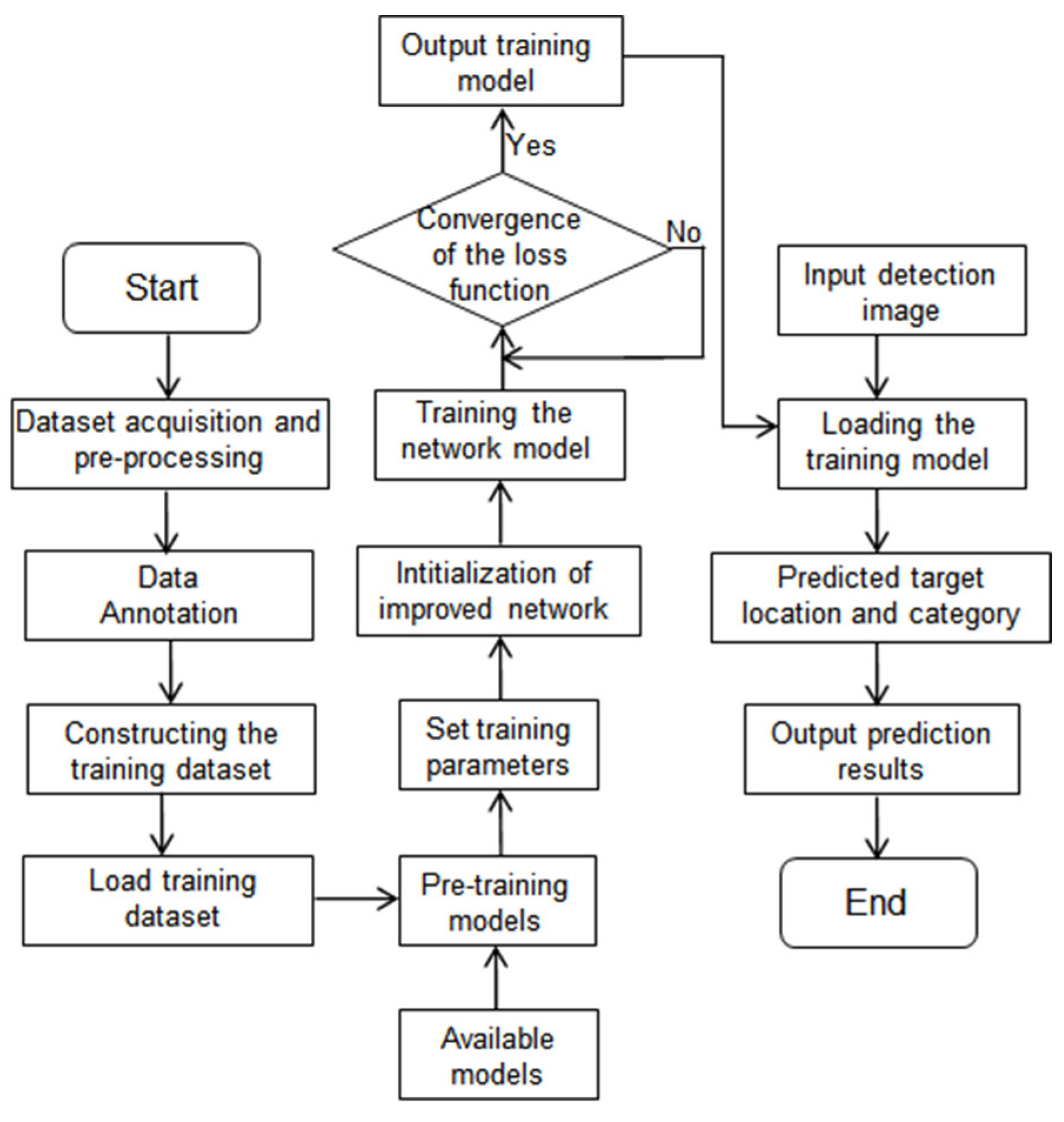
We proposed a tea tree pest detection model based on Yolov7-tiny. The experimental process is shown in Figure 1.
2.1.1. Yolov7-Tiny Algorithm
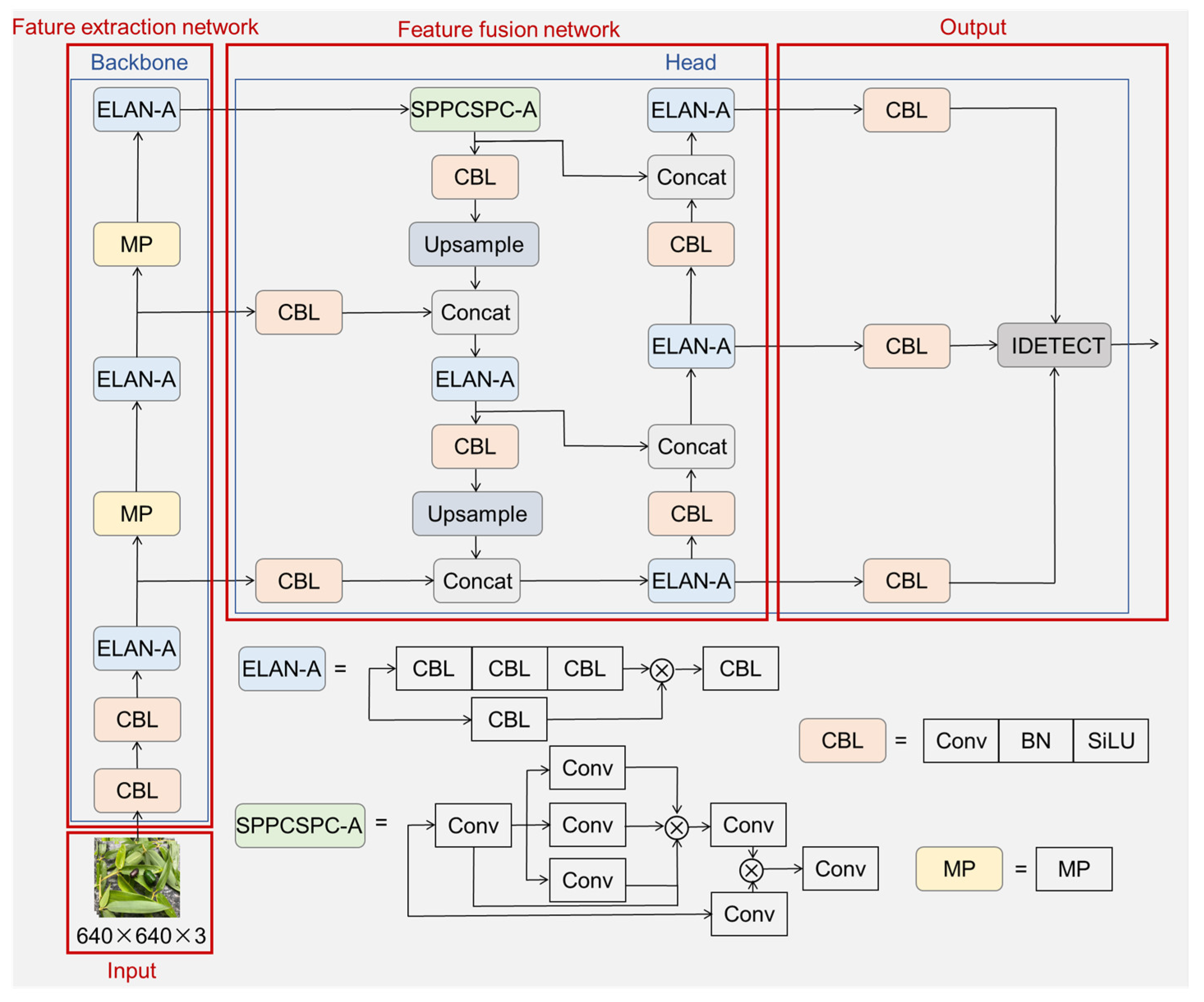
The Yolov7-tiny algorithm is derived from Yolov7, while retaining the cascade-based model scaling strategy and improving the efficient long-range aggregation network (ELAN) for improved detection accuracy with fewer parameters and faster detection speed. This makes it well-suited for tea tree pest detection requirements. The Yolov7-tiny algorithm is chosen as the basis for improvement. It consists of four parts: input, feature extraction network, feature fusion network, and output, as illustrated in Figure 2.
Feature extraction network: The feature extraction network includes CBL convolutional blocks, an improved efficient long-range aggregation network (ELAN-A) layer, and MPConv convolutional layer. While the ELAN-A layer enhances feature extraction speed, it may reduce the feature extraction capability as it cuts two sets of feature computation blocks from the original Yolov7.
Feature fusion network: The feature fusion network of Yolov7-tiny adopts the Path Aggregation Feature Pyramid Network (PAFPN) architecture from the Yolov5 series, which combines the strong semantic information from the top level of the Feature Pyramid Network (FPN) with the strong localization information tensor from the bottom-up of the Path Aggregation Network (PANet) to achieve multi-scale learning through feature information fusion [30,31]. However, the tensor splicing in Yolov7-tiny’s feature fusion network may not be comprehensive enough for fusing feature information of adjacent layers, and the nearest neighbor interpolation upsampling may not effectively balance the trade-off between speed and accuracy in the pest detection task. Additionally, the fusion network may not adequately prioritize the target feature information, which could result in feature information loss.
Output: The output of the proposed model uses an IDetect detection header [32], similar to the YoloR model, but introduces an implicit representation strategy to refine the prediction results based on fused feature values. However, the current detection header in Yolov7-tiny uses ordinary convolution, which may result in the detection of feature fusion results that do not focus on the expected target and which lacks a targeted strategy to improve the performance of small target detection.
Model prediction module: In the experimental dataset, there are images with two or more similar targets that are too close to each other. When using the traditional non-maximal suppression (NMS) algorithm for target classification and regression, these targets may be suppressed because their confidence score is lower than the maximum confidence score, resulting in missed detections.
2.1.2. Improved Yolov7-Tiny Tea Tree Pest Detection Algorithm
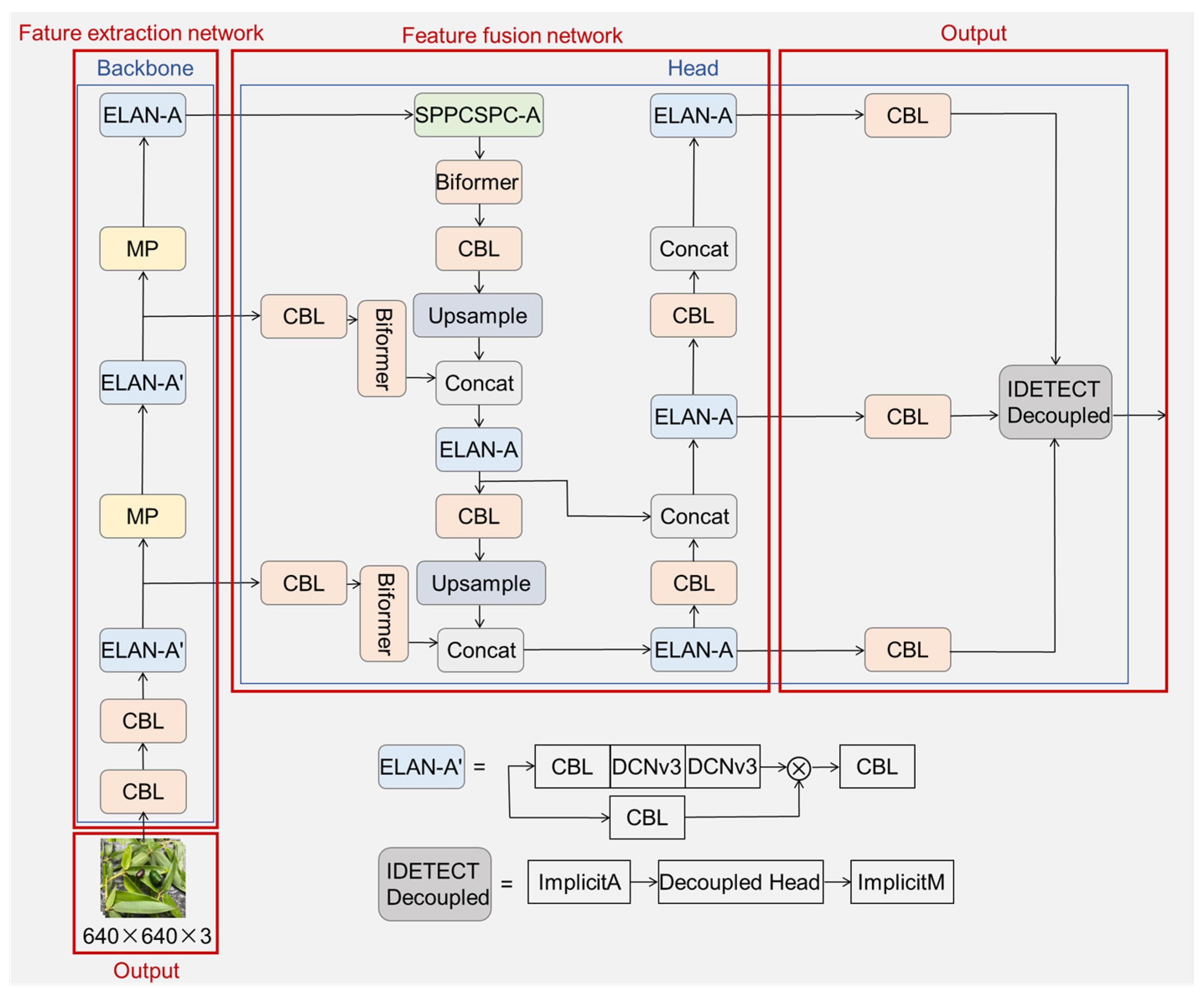
In order to enable Yolov7-tiny algorithm to more accurately detect the location of tea tree pests and accurately identify pest species, we propose improvements for each of the above deficiencies. We propose a common tea tree pest detection model based on the improved Yolov7-tiny algorithm, as illustrated in Figure 3.
To enhance the feature extraction capability of the model, deformable convolution is used in the feature extraction module to replace normal convolution. In addition, the Biformer dynamic attention mechanism is incorporated into the feature fusion module to capture more features with less computation. A new implicit decoupling head is also designed to reduce the extra delay overhead caused by the general decoupling head while improving accuracy. Finally, the soft-NMS algorithm is used to replace the NMS algorithm in the prediction module, which helps address the issues of wrong, multiple, and missed detections to some extent.
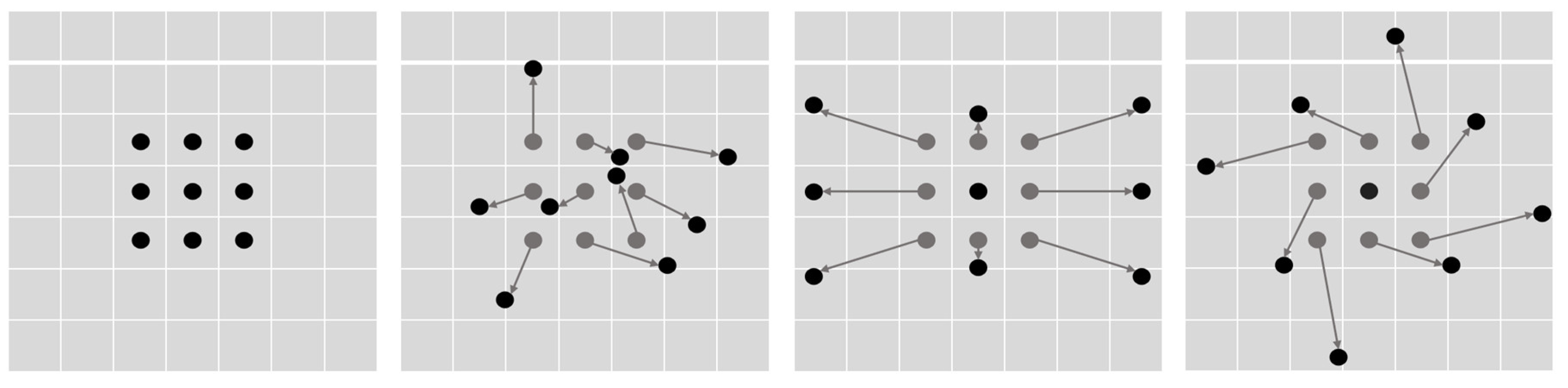
Improvements to the Feature Extraction Network: Deformable convolution (DCNv3) is utilized in the feature extraction module to replace normal convolution and enhance the feature extraction capability of the model [33,34,35]. The shape of the convolution kernel in deformable convolution is not fixed but rather can be changed adaptively based on the content of the target in the image. This flexible mapping allows for better coverage of the appearance of the detected target, thereby capturing more useful feature information. The complete representation of the DCNv3 operator is shown in Formula (1).
In Formula (1), G represents the number of groups, wg denotes the shared projection weight within each group, and mgk represents the normalized modulation factor of the kth sample point of the gth group. The DCNv3 operator addresses the limitations of traditional convolution in terms of long-range dependence and adaptive spatial aggregation, making it more suitable for large visual models. It achieves sparse global modeling while preserving the CNN, which allows for a better trade-off between computational effort and accuracy. Figure 4 depicts the different representations of deformable convolution.
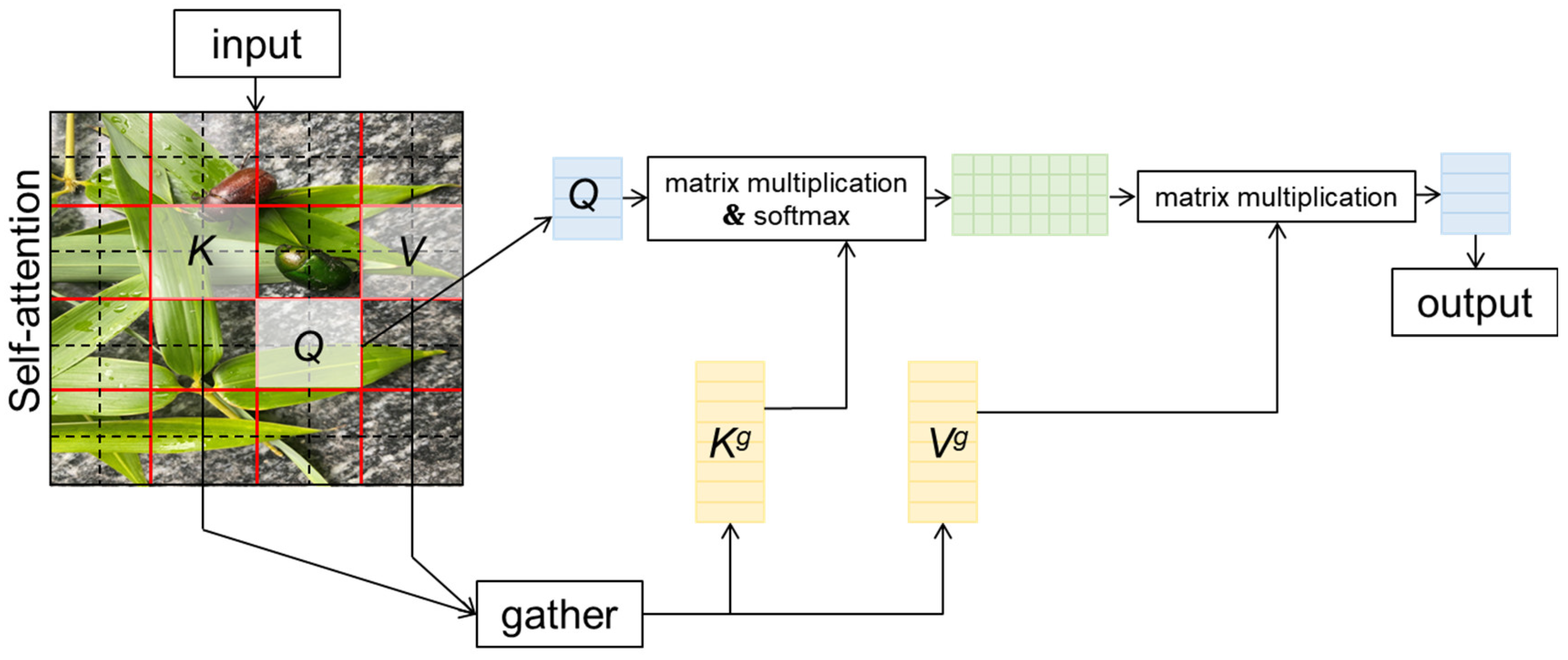
Improvements to Feature Fusion Networks: The Biformer dynamic attention mechanism is incorporated into the feature fusion module to achieve more flexible computational allocation and feature perception [36]. Biformer is a variant of the Transformer model that introduces a dynamic attention mechanism in the original Transformer model [37]. The dynamic attention mechanism adaptively adjusts the attention weights according to the features of the input image, so that different locations or features can be given different levels of attention, and the intensity and scope of attention can be flexibly controlled by adjusting the dynamic mask. The structure diagram of the Biformer dynamic attention mechanism is shown in Figure 5.
Q, K, V are to obtain the most relevant key-value pairs in a coarse region level so that only a small portion of routed regions remain. Then apply fine-grained token-to-token attention (Kg, Vg) in the union of these routed regions.
where Kg, Vg are gather key and value tensor. Ir means that the ith row contains k indices of the most relevant regions for ith region. The k represents gathering key-value pairs in the top k-related windows.
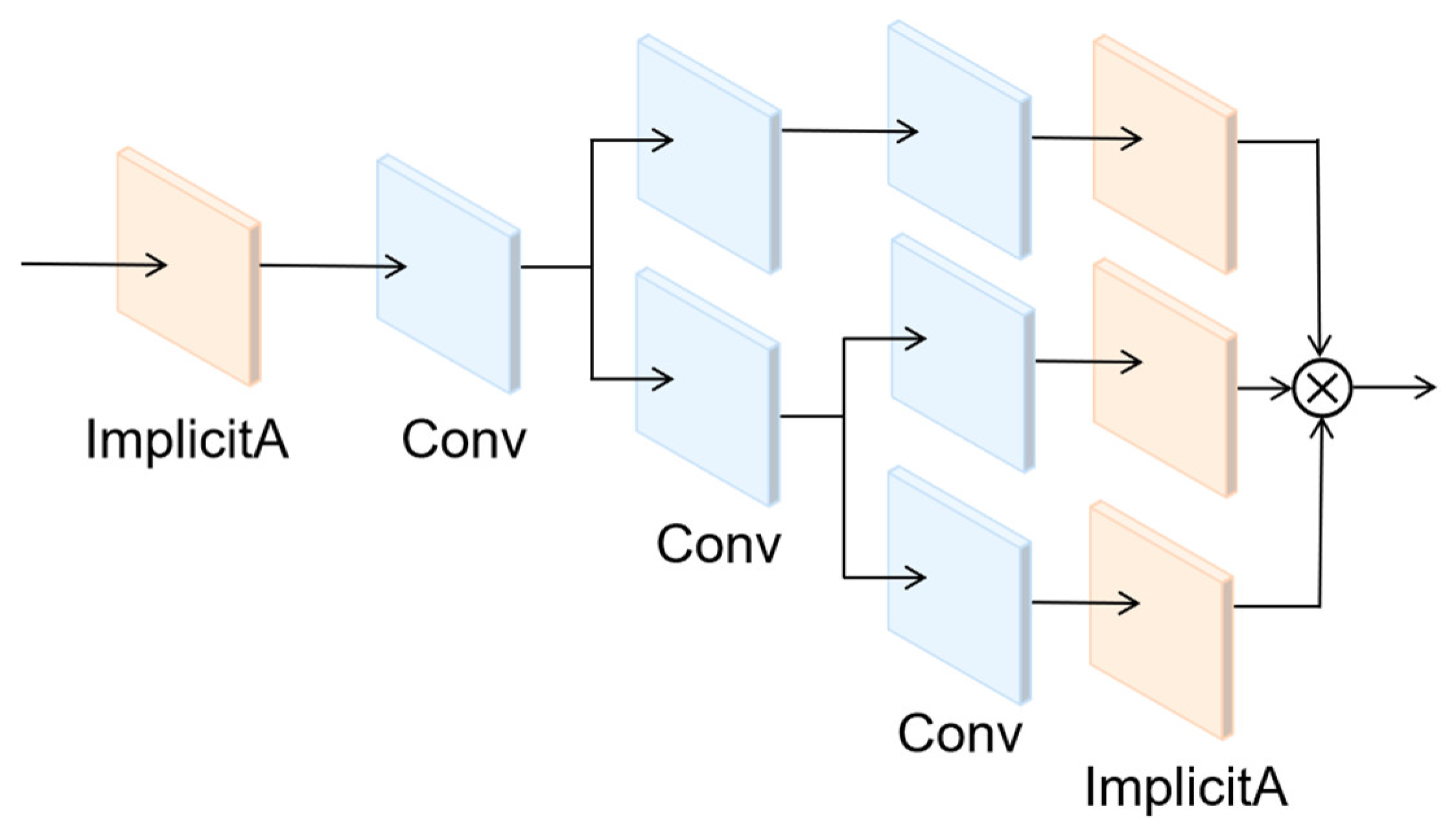
Improvements to the Output: A new implicit decoupling head (IDetect_Decoupled) is proposed at the output, which incorporates the implicit knowledge learning mentioned in YoloR into the decoupling detection head of Yolov6 [38]. This helps to further reduce the extra delay overhead caused by the general decoupling header while improving accuracy. The structure of this decoupling header is shown in Figure 6.
Model Prediction: Non-Maximal Suppression (NMS) is a crucial step in object detection. It ranks all detected bounding boxes based on their confidence scores, selects the box with the highest score as the maximum box, and suppresses the remaining boxes with significant overlap based on predefined confidence thresholds. This helps to obtain the final prediction result. However, in cases where multiple similar objects overlap in an image, boxes with scores lower than the highest score may be suppressed, resulting in missed detections. To address this issue, a continuous confidence suppression function is introduced in traditional NMS, known as soft-NMS [39]. Soft-NMS suppresses the confidence scores of non-maximal boxes to different degrees based on the size of the overlapping Intersection over Union (IoU) between non-maximal boxes and the maximum box. There are two expressions for soft-NMS: one is linearly weighted, as shown in Formula (4), and the other is Gaussian weighted, as shown in Formula (5).
In the equations mentioned above, Si represents the predictor box results that are retained, A represents the predictor box with the highest score, Bi represents the predictor boxes that are similar to the predictor box with the highest score, iou represents the intersection over union (IoU) ratio, Nt denotes the preset overlap threshold.
The above function will decay the detection score above Nt into A linear function that overlaps with A, so the detection box away from A will not be affected, and the detection box very close to A will be penalized more. However, it is not continuous in terms of overlap, and a sudden penalty is used when Nt’s NMS threshold is reached. It would be ideal if the penalty function were continuous, otherwise it would cause a sudden change in the sequence of checks. The continuous penalty function has no penalty when there is no overlap and a high penalty when there is high overlap. In addition, the penalty value should gradually increase when the overlap is low, because A should not affect the score of boxes with very little overlap. However, when the overlap between Bi and A approaches 1, Bi should be penalized significantly. Taking this into account, the updating pruning steps and Gaussian penalty function are proposed as follows:
where, σ denotes the standard deviation. This update rule is applied to each iteration and updates the scores of all remaining check boxes.
2.1.3. Class Activation Mapping
Class Activation Map (CAM) maps the response size of the feature Map to the original map so that the reader can more intuitively understand the effect of the model. CAM is the weighted linear sum of these visual patterns at different spatial locations. By sampling the CAM up to the size of the input image, we can identify the areas of the image that are most relevant to a particular category.
First, the images are input into the trained model and the results are recognized. Next obtain the layer that we want to have for the visual feature map. Then, the single channel or multi-channel feature map obtained in the first step is selected by a slicing method. The feature map is then resized to the size of the original image so that it can be overlaid with the original image. Next, the feature map generates a false color image based on the size of each element. Finally, the original image is superimposed onto the false-color image.
2.1.4. Mosaic
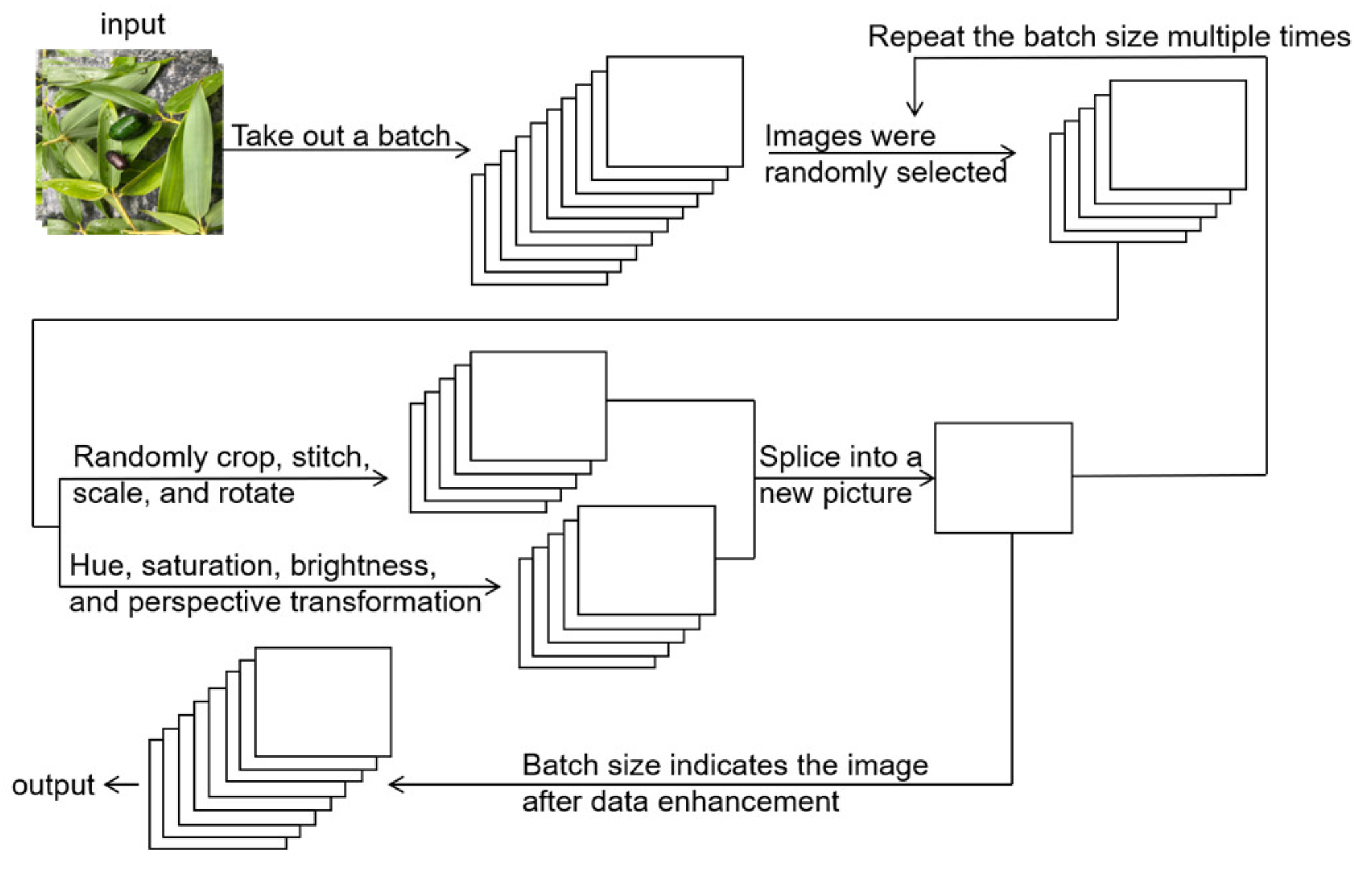
The flow chart of Mosaic technology is shown in Figure 7.
Mosaic technology is a data enhancement operation based on image transformation, which works by dividing the original image into a series of small pieces and then reassembling these pieces together, which may change position, size, and shape to form a new image. The whole process can simulate real visual changes, such as rotation, scaling, movement, etc., so as to obtain more information from the original image, thus better improving the generalization ability of the model.
2.1.5. Evaluation Indexes for Detection Model
We use precision (P), recall (R), average precision (AP), F1 Score (F1), and mean average precision (mAP), and all of these techniques were used as the metrics for evaluation.
Precision is defined as the correct detection rate of all detected targets, which can be expressed as Formula (4). TP represents True Positive, which is the number of targets detected by correct identification, and FP represents False Positive, which is the number of missed and wrong detections where the sample is judged as positive, but in fact it is negative.
Recall is defined as the correct detection rate in all positive samples, which can be expressed as Formula (5). FN: False Negative, the sample is judged as negative, but in fact it is positive. FN is the number of target objects detected as other kinds of objects.
The F1 Score is a weighted average of the accuracy and recall of the model, with a maximum value of one and a minimum value of zero. A larger value means a better model.
In Formulas (4) and (5), the average accuracy AP is defined as the mean value of the accuracy rate under different recall rates, and it is the integral of the accuracy rate to the recall rate, which can be expressed as Formula (7).
mAP is the average value taken over AP, n represents the number of target types, and APi is the average accuracy rate of the ith target, which is calculated with Formula (8).
mAP0.5 is the average AP value when the intersection ratio (IOU) threshold is 0.5, n represents the number of target species, and AP0.5i is the average accuracy rate of the ith target when the intersection ratio threshold is 0.5, which is calculated with Formula (9).
2.1.6. Experimental Environment
2.2. Materials
2.2.1. Image Dataset Acquisition
We used a common tea tree pest dataset as the experimental object wherein image data of tea tree pests with varying backgrounds were collected. The data was obtained through self-capture and web crawling. The image set was captured by the rear camera of an iPhone 11, which consists of a 12-megapixel wide-angle lens with a 26 mm equivalent focus segment and a 12-megapixel ultra-wide-angle lens with a 13 mm equivalent focus segment. Images were collected for eight different categories of tea tree pests, capturing them from different angles and backgrounds under both indoor and outdoor lighting conditions. During the image acquisition process, shooting locations and angles were randomly selected to capture pests from multiple directions, angles, and distances. As pests were in motion during the shooting, some of the images may have the phenomenon of obscured pests.
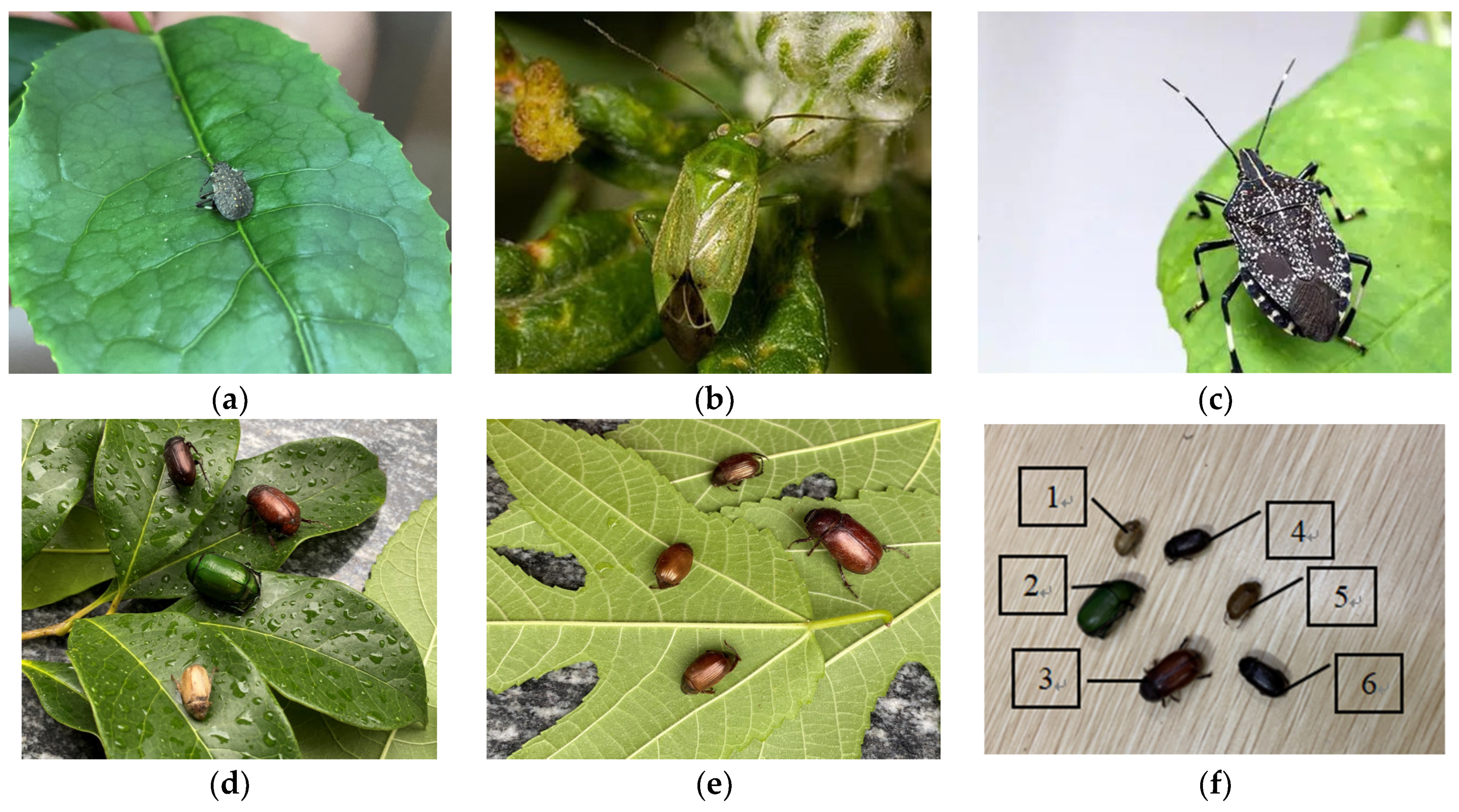
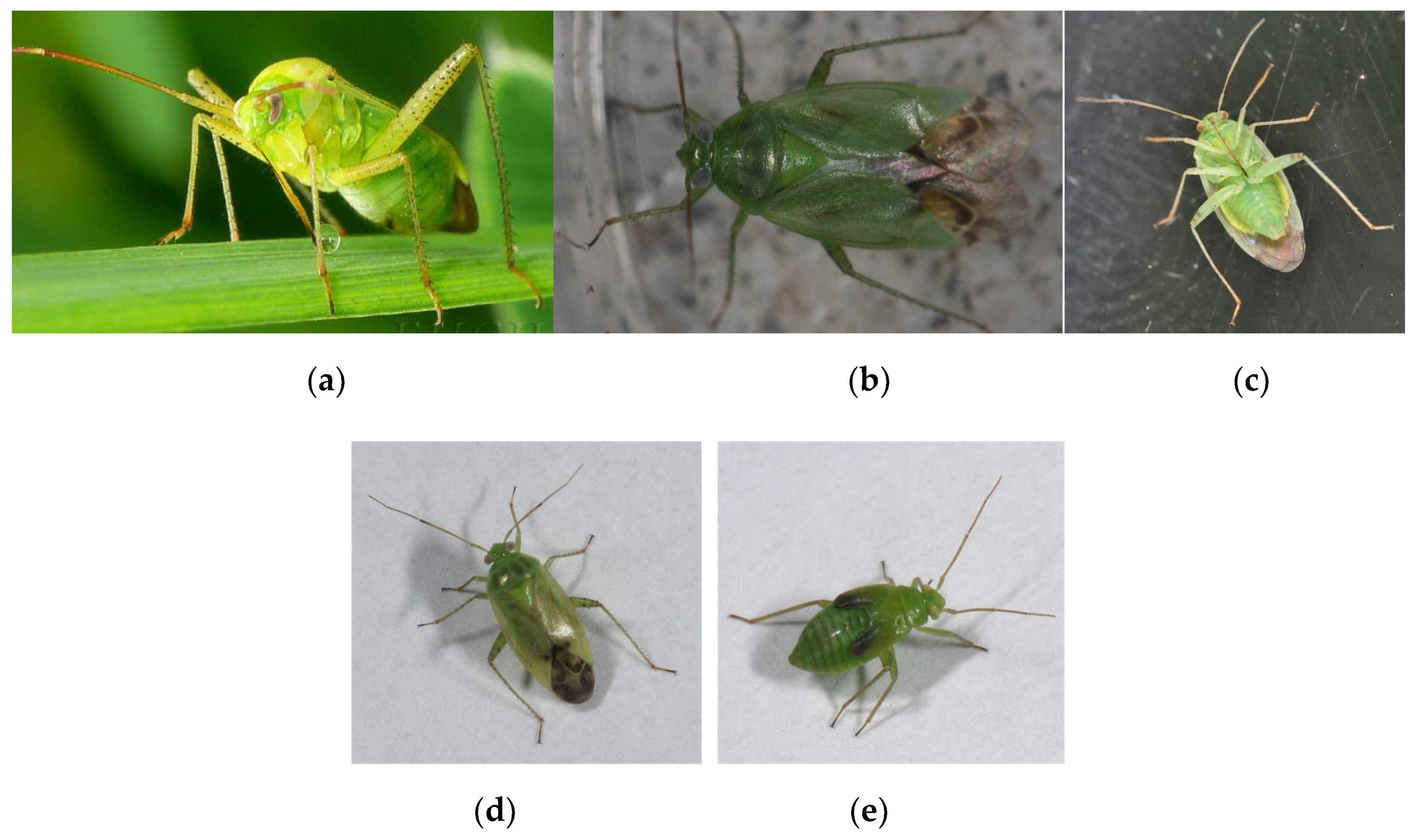
We used a common tea tree pest dataset as the experimental object. The data collection site was Hangzhou in July, and the number of scarab and bug pests was the largest component. Therefore, eight pests of scarab and bug species were selected as the main research objects in this experiment. Pest identification was performed by expert judgment opinion using species identification keys [40,41], including five species of scarab, namely Holotrichia parallela, Miridiba sinensis, Tawny beetle, Anomala corpulenta, and Proagopertha lucidula; as well as three species of bugs, namely Apolygus lucorum, Halyomorpha halys, and Erthesina fullo. The images of each type of pest are shown in Figure 8.
Figure 8a shows the images of Erthesina fullo taken by an iPhone11 in indoor lighting conditions. Figure 8b shows the images of Apolygus lucorum taken by an iPhone 11 in a real field environment. Figure 8c shows the image data of Halyomorpha halys obtained through online crawling (There is a pest called “Stinky Big sister”, which gives off a smell that is harmful to people, but has high medicinal value, 2021, digital photograph, https://baijiahao.baidu.com/s?id=1712052253063842078&wfr=spider&for=pc, accessed on 23 June 2022). Figure 8d shows the images of golden turtles taken under simulated real tea tree environments in outdoor lighting, with Holotrichia parallela, Miridiba sinensis, Anomala corpulenta, and Proagopertha lucidula from top to bottom. Figure 8e shows the images of golden turtles taken under simulated tea tree backgrounds in indoor lighting, with Tawny beetle on the left and larger Miridiba sinensis on the right. Figure 8f shows the dataset of golden turtle pests taken in a laboratory background under indoor lighting, with label one for Proagopertha lucidula, label two for Anomala corpulenta, label three for Miridiba sinensis, labels four and six for Holotrichia parallela, and label five for Tawny beetle.
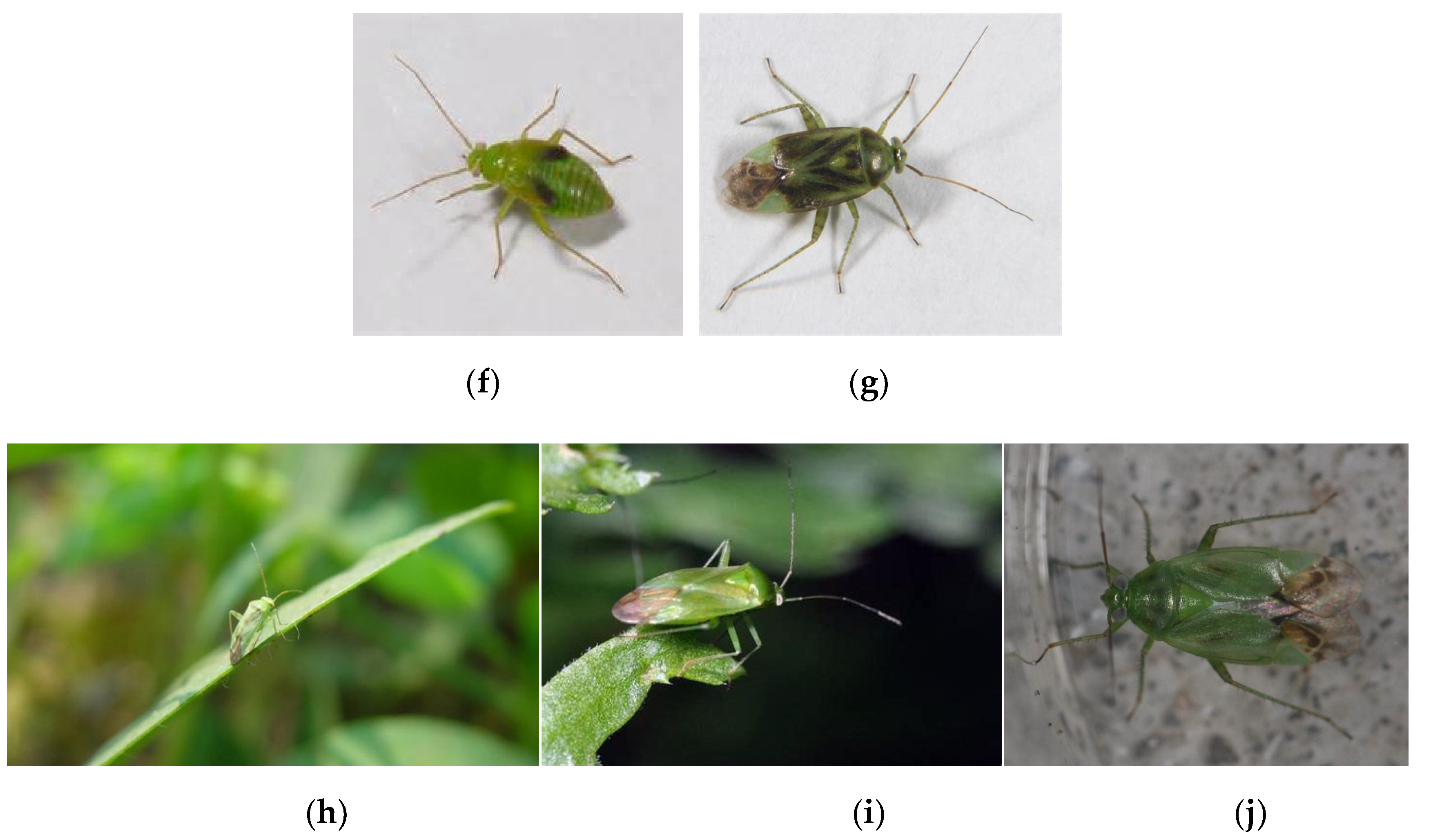
Taking the Apolygus lucorum images as an example, this dataset comprehensively includes detailed images of the pest from all angles, covering multi-angle, multi-direction, and multi-distance aspects, which requires adjustments to the model training. Figure 9a–c shows images of the Apolygus lucorum from different angles, Figure 9d–g shows images of the pest from different orientations, and Figure 9h–j shows images of the Apolygus lucorum from different distances.
The experimental data show the different poses of eight species of pests in real environments and indoor simulated environment backgrounds. This tea tree pest dataset collected a total of 782 image data, with each image randomly containing 1~5 different species of pests. Table 3 shows the occurrence times of various pests in the 782 images.
The size of the input image was fixed to 640 × 640 by using network adaptive scaling. The labeling tool was used for image labeling, generating txt files. The dataset was then segmented according to a 9:1 ratio and divided into two parts: train and val, which were used for training and testing of the model.
2.2.2. Data Enhancement
The model uses Mosaic to randomly crop, stitch, scale, and rotate 16 images. Additionally, hue, saturation, brightness, and the magnitude of perspective transformation are adjusted for each of the 16 images. Finally, an image is generated to be input into the network. The image processing methods and parameters are shown in Table 4.
The images processed as described above are then stitched into a single image, allowing the network to obtain information from 16 images simultaneously. This enriches the detection dataset while reducing the model’s difficulty in diversity learning. Moreover, during the process of random scaling, targets of different sizes are generated, which enhances the network’s robustness during continuous training and improves feature extraction. Finally, adaptive scaling anchor frames are used to scale the images to a uniform standard size, which is then fed into the network for detection.
3. Experimental Results
3.1. Model Optimizer Selection
In order to achieve better performance of the model, different optimizers were compared in this experiment to evaluate their effects on model performance. SGD and Adam are classical optimizers for optimizing the parameters of a model. The basic idea of SGD is to minimize the loss function of the model by constantly adjusting the parameters of the model through the method of gradient descent. Adam’s basic idea is to adjust the parameters of the model by maintaining the first and second order momenta of the model’s gradient and the square of the gradient. We thus compare the detection performance of the model under different learning rates of SGD optimizer and Adam optimizer, respectively. The adjustment of learning rate is achieved by manual adjustment, based on experience. The results of the different optimizer comparison experiments are shown in Table 5.
From the above table, we can see that when the model learning rate is 0.01 and 0.02, the SGD optimizer can better adapt to the model, and the correct rate is 91.6% and 91.5%, respectively; when the model learning rate is 0.001 and 0.002, the Adam optimizer has better performance, and the correct rate is 93.2% and 90.9%, respectively. The reason for the large difference in the above results is that SGD has the advantages of simple implementation and high efficiency, while its disadvantages are slow convergence speed and ease of falling into the local minimum. The advantages of Adam are high computational efficiency and fast convergence speed, while the disadvantages are finding suitable hyperparameters. The above data indicates that Adam optimizer is more suitable for this tea tree pest detection model, and Adam optimizer will be used in subsequent experiments and the learning rate will be set to 0.001.
Ablation Experiments
In order to better test and prove the performance of the model, ablation experiments are conducted. Based on the original Yolov7-tiny algorithm, only one improvement method is added at each step to verify the improvement effect of each improvement method on the original algorithm. A total of seven sets of experiments were performed to compare this model, and the results are shown in Table 6.
Yolov7-tiny is a simplified version of Yolov7, with 1.4% slightly lower accuracy compared to Yolov7, but with significantly reduced parameter calculations (only 1/7 of Yolov7). In order to make the model more suitable for popularization and application, this experiment is conducted by choosing Yolov7 with less parameter calculation. As can be seen from Table 4, the accuracy of the Yolov7-tiny network model with the addition of Biformer increased from 88.6% to 91.6% (+3%), and the recall rate increased from 86.2% to 89.3% (+3.1%). After replacing the convolution module with the dcnv3 convolution module, the mAP0.5 of the model improved from 88.6% to 91.2% (+2.6%), and the recall rate improved from 86.2% to 89.7% (+3.5%). When the model uses the IDetect_Decoupled detection algorithm instead of the original IDetect detection algorithm, mAP0.5 improves from 88.6% to 90.8% (+2.2%), and the recall rate improves from 86.2% to 89.9% (+3.7%). When the soft module was used in the NMS module of the model, the mAP0.5 of the model improved from 88.6% to 89.1% (+0.5%), and the recall rate improved from 86.2% to 91.6% (+5.4%). The mAP0.5 of the modified Improved Yolov7-tiny model improved from 88.6% to 92.2% (+3.6), and the recall rate improved from 90.45 to 96.85% (+6.40). The results show that the detection performance of pests in complex environments is slightly improved by continuous feature fusion, which improves the detection capability of the model and proves that the model can adapt to complex background environments.
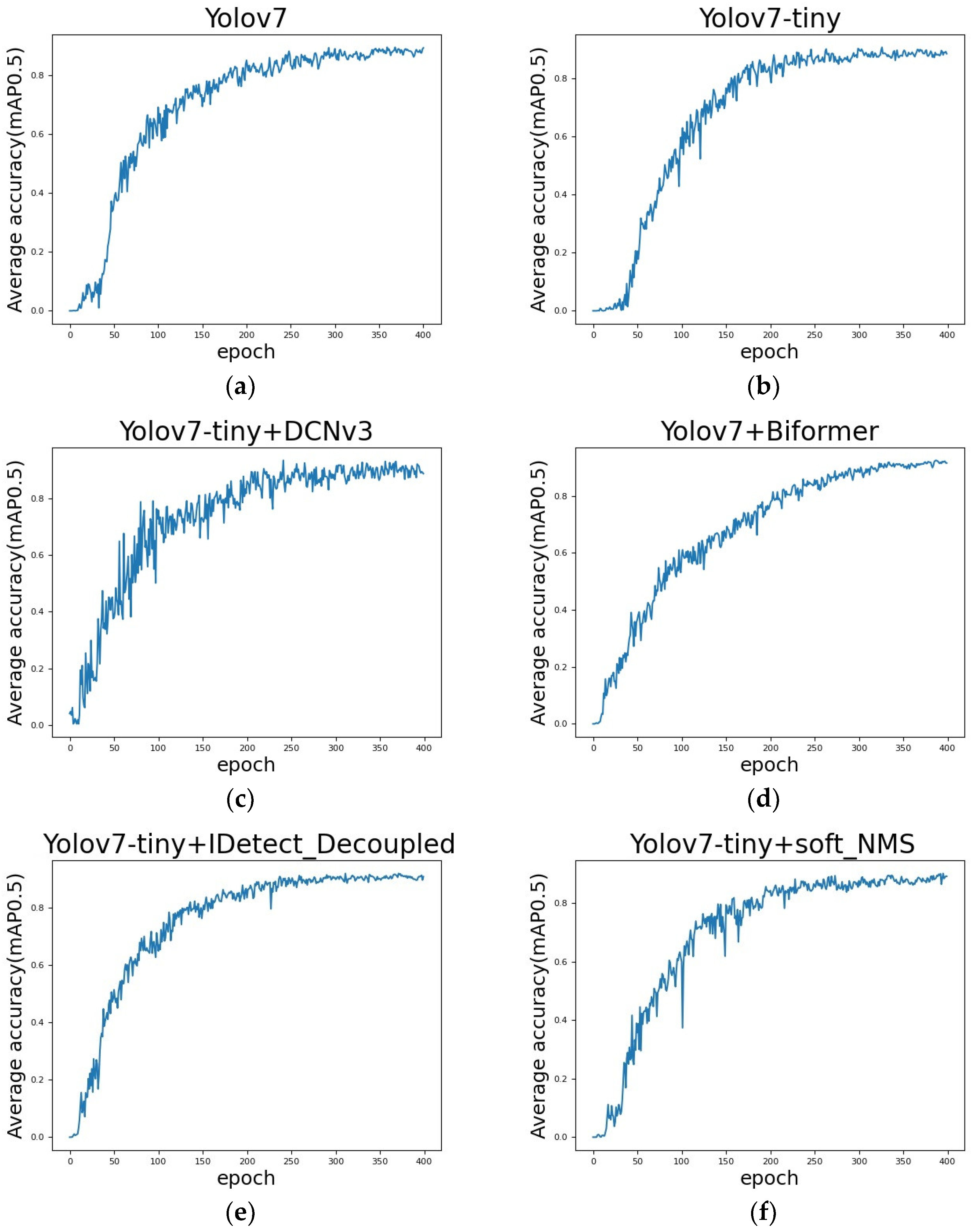
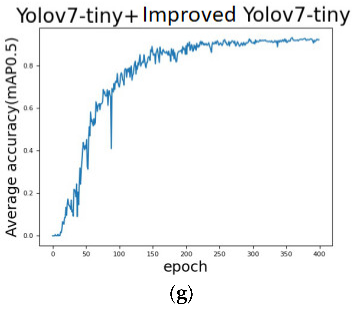
From Figure 10a,b, we can see that the Yolov7 algorithm starts to learn many image features at the tenth iteration during training, while Yolov7-tiny starts to learn image features only at the thirty-fifth iteration, and Yolov7 shows a convergence trend earlier than Yolov7-tiny, but both models start to be correct at 200 iterations leveling off. When the Biformer module, IDetect_Decoupled module, and soft_NMS module are added to the Yolov7-tiny model, respectively, they can make the Yolov7-tiny model extract the image feature information faster, but the correct rate of the DCNv3 module fluctuates significantly during detection, which indicates that the model does not recognize the feature information properly. The Biformer module has a slower convergence speed and requires a longer training time, but the data in Table 6 show that the introduction of the Biformer module can greatly improve the correct rate of model detection. The introduction of the IDetect_Decoupled module makes the network learn the features better, converge faster, and curve smoother. The improved Yolov7-tiny model starts to acquire a large amount of image feature information at the 12th iteration, convergence is completed at the 150th iteration, and the correct detection rate stabilizes at the 250th iteration. Compared with Yolov7-tiny, this model has faster convergence speed, higher accuracy, and a more stable detection rate.
As can be seen from Table 7, Improved Yolov7-tiny showed a higher improvement in the correct detection rate of Miridiba sinensis, from 78.8% to 94.3% (+15.5%). The Miridiba sinensis is similar to the Anomala corpulenta in body size, and similar to the Holotrichia parallela and Tawny beetle in color, so it led to the lower detection accuracy of Yolov7-tiny, but the Improved Yolov7-tiny improved its detection accuracy by 15.5%, indicating that Improved Yolov7-tiny can learn more feature information and distinguish them. The texture features of the Halyomorpha parallela are more complex, which are difficult to be captured and accurately identified from the complex background. The accuracy of Improved Yolov7-tiny increased from 78.8% to 84.9% (+6.2%), indicating that the improved model can better capture the detailed features of the pest and distinguish them from the complex background. The Apolygus lucorum color and background are so similar that it is difficult to distinguish them from the complex background, especially the tea tree background, while the accuracy of the improved model improved from 77.1% to 88.5% (11.4%). This indicates that the improved model can detect different types of similar pests in different complex backgrounds and improve the detection accuracy of fuzzy targets.
3.2. Performance Comparison of Different Models
To compare the performance of the modified Improved Yolov7-tiny network with other commonly used object detection models, several popular models including Efficientdet [42], Faster R-CNN [43], RetinaNet [44], DetNet [45], YOLO5s, YOLO-R, Yolov6, and Improved Yolov7-tiny were also built. All models were trained for 400 iterations. The comparison results are shown in Table 8.
As shown in Table 7, the model established by the algorithm exhibits higher accuracy and recall rate compared to other detection models. These results indicate that the proposed model improves performance to a certain extent, reducing the occurrence of errors and missed detections.
3.3. Comparison of Model Predictions
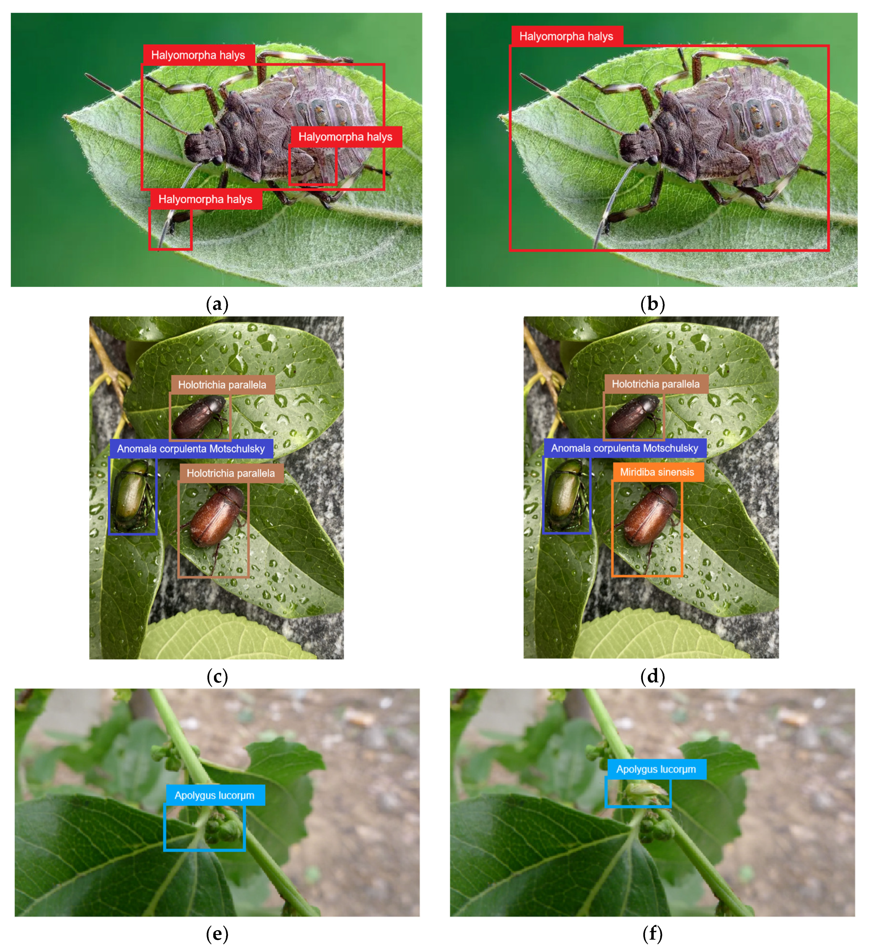
The test results of Yolov7-tiny and Improved Yolov7-tiny are visualized in an image visualization. The model output results are shown in Figure 11.
Figure 11a,c,e, respectively, show the phenomenon of multi-detection, wrong detection, and missing detection of the Yolov7-tiny model in pest detection. Figure 11b,d,f, respectively, show the improved detection results of the Yolov7-tiny model in corresponding images. In Figure 9a, due to the complex and similar texture of the back of the Halyomorpha halys, Yolov7-tiny mistakenly detected the same pest as three different pests. In Figure 11c, Yolov7-tiny mistakenly identified the Miridiba sinensis as the Holotrichia parallela because its color is similar to that of the black gill beetle. In Figure 11e, because the color of Apolygus lucorum is very similar to the background color and the background environment texture is complex, Yolov7-tiny misidentified the background information as Apolygus lucorum and defaults Apolygus lucorum as the background information. In Figure 11b,d,f, the Improved Yolov7-tiny model not only correctly detects the positions of all kinds of pests, but also correctly identifies the types of all kinds of pests.
3.4. Characteristic Heat Map
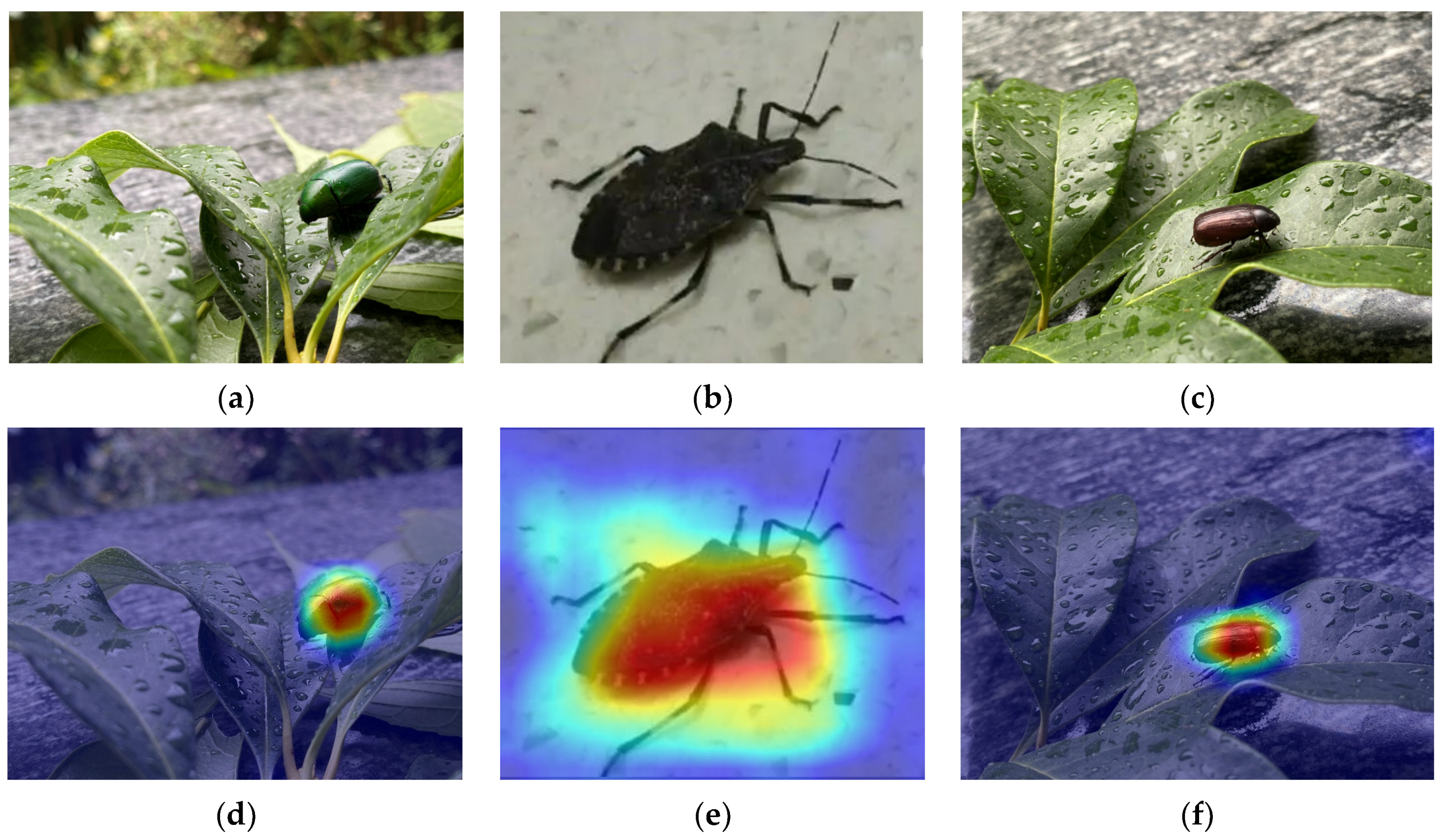
We randomly selected three images of different pests from the tea garden pest dataset and visualized the output features of the improved Yolov7-tiny using the Class Activation Mapping (CAM) algorithm. The computed results of the hidden layer feature maps for the corresponding samples from the trained Improved Yolov7-tiny model are shown in Figure 11. In the visualization, red color indicates the highest contribution, while blue color indicates the lowest contribution.
As shown in Figure 12a–c are the original images of the randomly selected Anomala corpulenta, Erthesina fullo, and Holotrichia parallela in the tea tree dataset, respectively. Figure 12d–f shows the focus areas of the Improved Yolov7-tiny model for feature extraction of these three pests, respectively. Through CAM, we can see that the locations focused on by the Improved Yolov7-tiny model are all located in the pests themselves. The results show that the Improved Yolov7-tiny model is able to accurately capture the features of the pests in the tea garden pest dataset.
4. Discussion
- The DCNv3 module enables Yolov7-tiny to have a faster convergence rate, so that the model can learn the feature information in the image faster. In the convolution process, the Yolov7-tiny model tends to pay more attention to the texture information of the image, while ignoring the background information, which makes the feature information finally extracted not rich enough. The DCNv3 module borrows the idea of depth-separable convolution to reduce the complexity of the DCN operator, using a shared weighted wg for projection. The same weight is used to project the sampling points, and then a position-aware learnable coefficient is used to weight the projected feature vectors. The DCN V3 operator makes up for the shortcomings of traditional convolution in long range dependence and adaptive spatial aggregation. While realizing sparse global modeling, it also appropriately retains the induction bias of CNN, which can be said to be a better balance between computational amount and accuracy. Therefore, the addition of the DCNv3 module makes the Yolov7-Tiny model more sensitive to image features, but its calculated parameters only increase by 0.5 MB compared with yolov7. However, it can be seen from Figure 10c that the average accuracy curve of the yolov7-tiny model fluctuates greatly after the introduction of DCNv3. Although the DCNv3 module can help the model to extract image features more quickly, it has certain limitations in feature recognition, resulting in large fluctuations in model recognition accuracy. We thus continue to improve the feature fusion module of Yolov7-tiny and the output side.
- The introduction of the Biformer dynamic attention mechanism and the IDetect_decoupled module makes smooth the average accuracy curve of the yolov7-tiny model, and the map of the model is improved after the introduction of the two modules, respectively. This shows that these two modules can enhance the feature recognition ability of the yolov7-tiny model. This may be because the Biformer dynamic attention mechanism saves parameters and computation by collecting key-value pairs in the first k-relevant windows and using sparsity operations to directly skip the calculation of the least relevant region. Since the module is based on sparse sampling rather than downsampling, it can better retain fine-grained details. In the convolutional neural network of the original model, the location information of pests with similar body types is partially lost, which affects the information fusion of the subsequent multi-scale feature pyramid, and thus leads to the omission of some pests. By adding the Biformer dynamic attention mechanism, Improved Yolov7-tiny can focus on the pest information in the image earlier, making the generated feature map information more abundant and improving the representation ability of the model. The IDetect_decoupled module is designed to incorporate the implicit knowledge learning mentioned in YoloR into Yolov6′s decoupled detection header. The decoupling head of YOLO V6 is based on the decoupling head of YOLO X to reduce the two convolutions of the YOLO X decoupling head into one convolution, which can shorten the training and testing time, but there will be some loss of accuracy. Therefore, on the basis of the YOLO V6 decoupled head, it is proposed to decouple its feature recognition ability by incorporating implicit knowledge learning. Yolov7-tiny+IDetect_Decoupled model has shown that its decoupled module can be decoupled to enhance the ability of the model.
- From the dataset, it can be observed that the Erthesina fullo pests are small in size, requiring the model to be capable of extracting features from small targets; the color characteristics of Apolygus lucorum are similar to the background environment, posing challenges for detection and classification; the Halyomorpha halys have complex texture characteristics, making them difficult to distinguish in complex backgrounds; the Miridiba sinensis, Tawny beetle, and Proagopertha lucidula have similar colors under indoor lighting; the Miridiba sinensis and Holotrichia parallela have very similar colors under outdoor lighting, and the size of Miridiba sinensis is similar to that of Anomala corpulenta; and the size of Holotrichia parallela, Proagopertha lucidula, and Tawny beetle is similar. These similarities pose significant challenges for the model. Therefore, yolov7-tiny can exhibit problems of false detection, missed detection, and multiple detection. In order to avoid cases where the final output prediction box is deleted because it overlaps too much with the current object box, we replace the traditional NMS module with the Soft-NMS module. The advantage of the Soft-NMS module is that the score of the detection box in the adjacent area (where the IOU exceeds the threshold) is adjusted instead of completely suppressed, thus improving accuracy in cases of high retrieval rate. When multiple target boxes are detected around the same object, select the box with the highest score each time and suppress the boxes around it. The larger the IoU of the box with the highest score, the greater the degree of suppression. In general, the IoU of a box representing the same object will be larger than the IoU of another object’s box, so that the other object’s box will remain, and the same object’s box will be removed. Soft-NMS thus preserves overlapping objects to a greater extent.
- Therefore, we propose a tea garden pest detection model based on Yolov7-tiny. The model utilizes a deformable convolution network to replace normal convolution in the feature extraction module, enhancing the model’s capability for feature extraction. It also incorporates the Biformer dynamic attention mechanism in the feature fusion module, allowing for more flexible computational allocation and improved feature perception. Additionally, a new implicit decoupling head is proposed at the output side to reduce the extra delay overhead caused by the general decoupling head, while also improving accuracy. Lastly, the model’s prediction employs a softened non-maximal suppression algorithm approach instead of the original non-maximal suppression algorithm, addressing issues such as pest misdetection, omission, and multiple detection. The average accuracy of the Improved Yolov7-tiny model proposed by us reaches 93.23%, which is higher than other traditional deep learning detection models. The pest detection model proposed has promising application prospects and has the potential to reduce the time and economic cost of pest control in tea plantations.
5. Conclusions
Applying deep learning technology to the field of tea tree pest control has strong practical and research significance for improving pest control efforts. We propose a Yolov7-tiny-based pest detection model for tea plantations. The model replaces the normal convolution with deformable convolution in the feature extraction module and incorporates the Biformer dynamic attention mechanism in the feature fusion module, proposes a new implicit decoupling head to replace the original detection head, and uses a softened non-maximum suppression algorithm in the model prediction instead of the original non-maximum suppression algorithm. The average accuracy of the detection algorithm is 93.2%, which is 4.6% higher than Yolov7-tiny and 3.2% higher than Yolov7, and its parameter computation is only 2/7 of Yolov7. On the tea garden pest dataset, the proposed model demonstrates higher detection accuracy with reduced training time and computation compared to other common detection algorithms. Improved Yolov7-tiny can meet the needs of pest detection in complex environments, and because of its small number of parameters, it can achieve fast detection and is easy to promote and apply. This study has achieved some results on a dataset of tea tree pests, which has some reference value for tea tree pests. To further enhance the quality and impact of the research presented in this paper [46], we would like to consider including a paragraph on the use of formal methods for the verification of AI-based techniques in the next iteration. By utilizing formal methods, we can ensure that our techniques are robust, reliable, and free from errors or biases.
Author Contributions
Conceptualization, Z.Y.; Formal analysis, Z.Y.; Investigation, X.W.; Data curation, Y.R.; Funding acquisition, H.F.; Methodology, Z.Y.; Resources, H.F.; Writing—original draft, Z.Y.; Writing—review, Z.Y.; Visualization, Z.Y. All authors have read and agreed to the published version of the manuscript.
Funding
Key R&D Projects in Zhejiang Province (2022C02020); Three agricultural nine-party science and technology collaboration projects in Zhejiang Province (2022SNJF036); Basic Public Welfare Project in Zhejiang Province (GN21F020001).
Institutional Review Board Statement
Not applicable.
Data Availability Statement
The data presented in this study are available on request from the corresponding author.
Conflicts of Interest
The authors declare no conflict of interest.
References
- Xia, E.H.; Zhang, H.B.; Sheng, J.; Li, K.; Zhang, Q.J.; Kim, C.; Zhang, Y.; Liu, Y.; Zhu, T.; Li, W.; et al. The tea tree genome provides insights into tea flavor and independent evolution of caffeine biosynthesis. Mol. Plant 2017, 10, 866–877. [Google Scholar] [CrossRef]
- Wei, C.; Yang, H.; Wang, S.; Zhao, J.; Liu, C.; Gao, L.; Xia, E.; Lu, Y.; Tai, Y.; She, G.; et al. Draft genome sequence of Camellia sinensis var. sinensis provides insights into the evolution of the tea genome and tea quality. Proc. Natl. Acad. Sci. USA 2018, 115, E4151–E4158. [Google Scholar] [PubMed]
- Xia, E.H.; Tong, W.; Wu, Q.; Wei, S.; Zhao, J.; Zhang, Z.Z.; Wei, C.L.; Wan, X.C. Tea plant genomics: Achievements, challenges and perspectives. Hortic. Res. 2020, 7, 7. [Google Scholar] [PubMed]
- Lou, S.; Zhang, B.; Zhang, D. Foresight from the hometown of green tea in China: Tea farmers’ adoption of pro-green control technology for tea plant pests. J. Clean. Prod. 2021, 320, 128817. [Google Scholar]
- Cranham, J.E. Tea pests and their control. Annu. Rev. Entomol. 1966, 11, 491–514. [Google Scholar] [CrossRef]
- Pinhas, J.; Soroker, V.; Hetzroni, A.; Mizrach, A.; Teicher, M.; Goldberger, J. Automatic acoustic detection of the red palm weevil. Comput. Electron. Agric. 2008, 63, 131–139. [Google Scholar] [CrossRef]
- Hetzroni, A.; Soroker, V.; Cohen, Y. Toward practical acoustic red palm weevil detection. Comput. Electron. Agric. 2016, 124, 100–106. [Google Scholar] [CrossRef]
- Subramanyam, B.; Hagstrum, D.W. (Eds.) Alternatives to Pesticides in Stored-Product IPM; Springer US: New York, NY, USA, 2012. [Google Scholar]
- Larios, N.; Deng, H.; Zhang, W.; Sarpola, M.; Yuen, J.; Paasch, R.; Moldenke, A.; Lytle, D.A.; Correa, S.R.; Mortensen, E.N.; et al. Automated insect identification through concatenated histograms of local appearance features: Feature vector generation and region detection for deformable objects. Mach. Vis. Appl. 2008, 19, 105–123. [Google Scholar] [CrossRef]
- Yaakob, S.N.; Jain, L. An insect classification analysis based on shape features using quality threshold ARTMAP and moment invariant. Appl. Intell. 2012, 37, 12–30. [Google Scholar]
- Espinoza, K.; Valera, D.L.; Torres, J.A.; López, A.; Molina-Aiz, F.D. Combination of Image Processing and Artificial Neural Networks as a Novel Approach for the Identification of Bemisia Tabaci and Frankliniella Occidentalis on Sticky Traps in Greenhouse Agriculture. Comput. Electron. Agric. 2016, 127, 495–505. [Google Scholar] [CrossRef]
- Pujari, D.; Yakkundimath, R.; Byadgi, A.S. SVM and ANN based classification of plant diseases using feature reduction technique. IJIMAI 2016, 3, 6–14. [Google Scholar] [CrossRef]
- Thenmozhi, K.; Reddy, U.S. Image processing techniques for insect shape detection in field crops. In Proceedings of the 2017 International Conference on Inventive Computing and Informatics (ICICI), Coimbatore, India, 23–24 November 2017; IEEE: New York, NY, USA, 2017; pp. 699–704. [Google Scholar]
- Ebrahimi, M.A.; Khoshtaghaza, M.H.; Minaei, S.; Jamshidi, B. Vision-based pest detection based on SVM classification method. Comput. Electron. Agric. 2017, 137, 52–58. [Google Scholar]
- Krizhevsky, A.; Sutskever, I.; Hinton, G.E. Imagenet classification with deep convolutional neural networks. Commun. ACM 2017, 60, 84–90. [Google Scholar] [CrossRef]
- Geiger, A.; Lenz, P.; Urtasun, R. Are we ready for autonomous driving? The kitti vision benchmark suite. In Proceedings of the 2012 IEEE Conference on Computer Vision and Pattern Recognition, Providence, RI, USA, 16–21 June 2012; IEEE: New York, NY, USA, 2012; pp. 3354–3361. [Google Scholar]
- Dai, X. HybridNet: A fast vehicle detection system for autonomous driving. Signal Process. Image Commun. 2019, 70, 79–88. [Google Scholar]
- Wu, Y.; Jiang, B.; Lu, N. A descriptor system approach for estimation of incipient faults with application to high-speed railway traction devices. IEEE Trans. Syst. Man Cybern. Syst. 2017, 49, 2108–2118. [Google Scholar]
- Wu, Y.; Jiang, B.; Wang, Y. Incipient winding fault detection and diagnosis for squirrel-cage induction motors equipped on CRH trains. ISA Trans. 2020, 99, 488–495. [Google Scholar]
- Li, Z.; Dong, M.; Wen, S.; Hu, X.; Zhou, P.; Zeng, Z. CLU-CNNs: Object detection for medical images. Neurocomputing 2019, 350, 53–59. [Google Scholar]
- Lee, S.G.; Bae, J.S.; Kim, H.; Kim, J.H.; Yoon, S. Liver lesion detection from weakly-labeled multi-phase ct volumes with a grouped single shot multibox detector. In Proceedings of the Medical Image Computing and Computer Assisted Intervention–MICCAI 2018: 21st International Conference, Proceedings, Part II 11, Granada, Spain, 16–20 September 2018; Springer International Publishing: Berlin/Heidelberg, Germany, 2018; pp. 693–701. [Google Scholar]
- Kamilaris, A.; Prenafeta-Boldú, F.X. Deep learning in agriculture: A survey. Comput. Electron. Agric. 2018, 147, 70–90. [Google Scholar]
- Zhu, N.; Liu, X.; Liu, Z.; Hu, K.; Wang, Y.; Tan, J.; Huang, M.; Zhu, Q.; Ji, X.; Jiang, Y.; et al. Deep learning for smart agriculture: Concepts, tools, applications, and opportunities. Int. J. Agric. Biol. Eng. 2018, 11, 32–44. [Google Scholar] [CrossRef]
- Shen, Y.; Zhou, H.; Li, J.; Jian, F.; Jayas, D.S. Detection of stored-grain insects using deep learning. Comput. Electron. Agric. 2018, 145, 319–325. [Google Scholar]
- Li, R.; Wang, R.; Xie, C.; Liu, L.; Zhang, J.; Wang, F.; Liu, W. A coarse-to-fine network for aphid recognition and detection in the field. Biosyst. Eng. 2019, 187, 39–52. [Google Scholar]
- Tetila, E.C.; Machado, B.B.; Astolfi, G.; de Souza Belete, N.A.; Amorim, W.P.; Roel, A.R.; Pistori, H. Detection and classification of soybean pests using deep learning with UAV images. Comput. Electron. Agric. 2020, 179, 105836. [Google Scholar]
- Chen, J.; Chen, W.; Zeb, A.; Zhang, D.; Nanehkaran, Y.A. Crop pest recognition using attention-embedded lightweight network under field conditions. Appl. Entomol. Zool. 2021, 56, 427–442. [Google Scholar]
- Chu, J.; Li, Y.; Feng, H. Research on Multi-Scale Pest Detection and Identification Method in Granary Based on Improved YOLOv5. Agriculture 2023, 13, 364. [Google Scholar]
- Wang, J.; Li, Y.; Feng, H.; Ren, L.; Du, X.; Wu, J. Common pests image recognition based on deep convolutional neural network. Comput. Electron. Agric. 2020, 179, 105834. [Google Scholar]
- Liu, S.; Qi, L.; Qin, H.; Shi, J.; Jia, J. Path aggregation network for instance segmentation. In Proceedings of the IEEE Conference on Computer Vision and Pattern Recognition, Salt Lake City, UT, USA, 18–23 June 2018; pp. 8759–8768. [Google Scholar]
- Wang, C.Y.; Yeh, I.H.; Liao, H.Y.M. You only learn one representation: Unified network for multiple tasks. arXiv 2021, arXiv:2105.04206. [Google Scholar]
- Dai, J.; Qi, H.; Xiong, Y.; Li, Y.; Zhang, G.; Hu, H.; Wei, Y. Deformable convolutional networks. In Proceedings of the IEEE International Conference on Computer Vision, Venice, Italy, 22–29 October 2017; pp. 764–773. [Google Scholar]
- Zhu, X.; Hu, H.; Lin, S.; Dai, J. Deformable convnets v2: More deformable, better results. In Proceedings of the IEEE/CVF Conference on Computer Vision and Pattern Recognition, Long Beach, CA, USA, 15–20 June 2019; pp. 9308–9316. [Google Scholar]
- Yang, Z.; Liu, S.; Hu, H.; Wang, L.; Lin, S. Reppoints: Point set representation for object detection. In Proceedings of the IEEE/CVF International Conference on Computer Vision, Seoul, Republic of Korea, 27 October–2 November 2019; pp. 9657–9666. [Google Scholar]
- Zhu, L.; Wang, X.; Ke, Z.; Zhang, W.; Lau, R. BiFormer: Vision Transformer with Bi-Level Routing Attention. arXiv 2023, arXiv:2303.08810. [Google Scholar]
- Vaswani, A.; Shazeer, N.; Parmar, N.; Uszkoreit, J.; Jones, L.; Gomez, A.N.; Kaiser, Ł.; Polosukhin, I. Attention is all you need. Adv. Neural Inf. Process. Syst. 2017, arXiv:1706.03762. [Google Scholar]
- Li, C.; Li, L.; Jiang, H.; Weng, K.; Geng, Y.; Li, L.; Ke, Z.; Li, Q.; Cheng, M.; Nie, W.; et al. YOLOv6: A single-stage object detection framework for industrial applications. arXiv 2022, arXiv:2209.02976. [Google Scholar]
- Bodla, N.; Singh, B.; Chellappa, R.; Davis, L.S. Soft-NMS--improving object detection with one line of code. In Proceedings of the IEEE International Conference on Computer Vision, Venice, Italy, 22–29 October 2017; pp. 5561–5569. [Google Scholar]
- Guangrui, L.; Youwei, Z.; Rui, W. Color Map of Common Scarab in Northern China; China Forestry Publishing House: Changchun, China, 1997. [Google Scholar]
- Fabre. Entomology; Jilin Fine Arts Publishing House: Changchun, China, 2019. [Google Scholar]
- Tan, M.; Pang, R.; Le, Q.V. Efficientdet: Scalable and efficient object detection. In Proceedings of the IEEE/CVF Conference on Computer Vision and Pattern Recognition, Seattle, WA, USA, 13–19 June 2020; pp. 10781–10790. [Google Scholar]
- Ren, S.; He, K.; Girshick, R.; Sun, J. Faster r-cnn: Towards real-time object detection with region proposal networks. Adv. Neural Inf. Process. Syst. 2015, arXiv:1506.01497. [Google Scholar]
- Lin, T.Y.; Goyal, P.; Girshick, R.; He, K.; Dollár, P. Focal loss for dense object detection. In Proceedings of the IEEE International Conference on Computer Vision, Venice, Italy, 22–29 October 2017; pp. 2980–2988. [Google Scholar]
- Li, Z.; Peng, C.; Yu, G.; Zhang, X.; Deng, Y.; Sun, J. Detnet: A backbone network for object detection. arXiv 2018, arXiv:1804.06215. [Google Scholar]
- Krichen, M.; Mihoub, A.; Alzahrani, M.Y.; Adoni, W.Y.; Nahhal, T. Are Formal Methods Applicable to Machine Learning And Artificial Intelligence? In Proceedings of the 2022 2nd International Conference of Smart Systems and Emerging Technologies (SMARTTECH), Riyadh, Saudi Arabia, 9–11 May 2022; IEEE: New York, NY, USA, 2022; pp. 48–53. [Google Scholar]
- Raman, R.; Gupta, N.; Jeppu, Y. Framework for Formal Verification of Machine Learning Based Complex System-of-Systems. INSIGHT 2023, 26, 91–102. [Google Scholar] [CrossRef]
Figure 1.
The general flow chart of this paper.

Figure 2.
Structure of Yolov7-tiny.

Figure 3.
Structure of the improved Yolov7-tiny network model.

Figure 4.
Different representations of deformable convolution.

Figure 5.
The structure diagram of the Biformer dynamic attention mechanism.

Figure 6.
Structure of IDetect_Decoupled.

Figure 7.
The flow chart of Mosaic technology.

Figure 8.
Examples of common tea tree pest datasets. (a–c) are images of bug pests. (d–f) are images of scarab pests.
Figure 8.
Examples of common tea tree pest datasets. (a–c) are images of bug pests. (d–f) are images of scarab pests.

Figure 9.
Partial data images of Apolygus lucorum. (a) Head image. (b) Dorsal image. (c) Abdomen image. (d) Right rear shot of the bug. (e) Left front shot of the bug. (f) Right front shot of the bug. (g) Side and rear shot of the bug. (h) Long range. (i) Medium range. (j) Close range.
Figure 9.
Partial data images of Apolygus lucorum. (a) Head image. (b) Dorsal image. (c) Abdomen image. (d) Right rear shot of the bug. (e) Left front shot of the bug. (f) Right front shot of the bug. (g) Side and rear shot of the bug. (h) Long range. (i) Medium range. (j) Close range.


Figure 10.
Effect of different optimization algorithms on training.


Figure 11.
Identification of Yolov7-tiny and Improved Yolov7-tiny model results. (a) Yolov7-tiny assay result graph. (b) Improved Yolov7-tiny assay result graph. (c) Yolov7-tiny assay results. (d) Improved Yolov7-tiny assay results. (e) Yolov7-tiny assay results. (f) Improved Yolov7-tiny assay results.

Figure 12.
Example of Improved Yolov7-tiny hidden layer feature map. (a–c) are the original pest images of the three pests, and (d–f) are the class activation map images of the three pests.
Figure 12.
Example of Improved Yolov7-tiny hidden layer feature map. (a–c) are the original pest images of the three pests, and (d–f) are the class activation map images of the three pests.


Table 1.
Experimental environment configuration.
| Name | Configuration |
|---|---|
| GPU | RTX3090 |
| CPU | Core i9-10900K |
| CUDA | 11.1 |
| Memory | 128 G |
| Operating system | ubuntu22.04 LTS |
Table 2.
Experimental model parameters.
| Training Parameters Parameter | Values |
|---|---|
| Input image size | 640 × 640 |
| Batch size | 32 |
| Epochs | 400 |
| Momentum | 0.937 |
| Weight Decay | 0.0005 |
| Warm-up | 3.0 |
Table 3.
Number of occurrences of the different pest species.
| Pest Species | Holotrichia parallela | Miridiba sinensis | Tawny beetle | Anomala corpulenta | Proagopertha lucidula | Apolygus lucorum | Halyomorpha halys | Erthesina fullo |
|---|---|---|---|---|---|---|---|---|
| Occurrence | 342 | 357 | 369 | 345 | 356 | 134 | 115 | 118 |
Table 4.
Image processing methods and parameters.
| Adjustment Method | Parameters |
|---|---|
| Color Tones | 0.015 |
| Saturation | 0.7 |
| Brightness | 0.4 |
| Rotation angle | 90° |
| Magnitude of image panning | 0.2 |
| Magnitude of image scaling | 0.9 |
| Probability of flipping left and right | 50% |
| Probability of randomly stitching multiple images using mosaic technique | 100% |
| Probability of blending multiple images using mix-up technique | 15% |
| Probability of copying and pasting on a single image | 15% |
Table 5.
Comparison experimental results of different optimizers.
| Optimizer | Learning Rate | Average Accuracy (mAP0.5)/% |
|---|---|---|
| SGD | 0.01 | 91.6 |
| 0.001 | 63.2 | |
| 0.02 | 91.5 | |
| 0.002 | 84.3 | |
| Adam | 0.01 | 80.3 |
| 0.001 | 93.2 | |
| 0.02 | 75.6 | |
| 0.002 | 90.9 |
Table 6.
Ablation experiments.
| Model | Average Accuracy (mAP0.5)/% | Recall (R)/% | #Param. |
|---|---|---|---|
| Yolov7 | 90.0 | 91.5 | 74.8 MB |
| Yolov7-tiny | 88.6 | 86.2 | 12.3 MB |
| Yolov7-tiny+dcnv3 | 91.2 | 89.7 | 12.8 MB |
| Yolov7-tiny+Biformer | 91.6 | 89.3 | 12.8 MB |
| Yolov7-tiny + IDetect_Decoupled | 90.8 | 89.9 | 25.4 MB |
| Yolov7-tiny + soft-NMS | 89.1 | 91.6 | 12.3 MB |
| Improved Yolov7-tiny | 93.2 | 93.6 | 26.4 MB |
Table 7.
Comparison of detection accuracy of various pests before and after improvement.
| Model | Average Accuracy (%) | |||||||
|---|---|---|---|---|---|---|---|---|
| AP1 | AP2 | AP3 | AP4 | AP5 | AP6 | AP7 | AP8 | |
| Yolov7-tiny | 78.7 | 77.1 | 85.1 | 98.8 | 78.8 | 100 | 90.8 | 100 |
| Improved Yolov7-tiny | 84.9 | 88.5 | 86.6 | 98.7 | 94.3 | 100 | 92.6 | 100 |
Note: AP1 is the Halyomorpha halys; AP2 is the Apolygus lucorum; AP3 is the Erthesina fullo; AP4 is the Holotrichia parallela; AP5 is the Miridiba sinensis; AP6 is the Tawny beetle; AP7 is the Anomala corpulenta; AP8 is the Proagopertha lucidula.
Table 8.
Comparison of correct detection rates of different models.
| Model | Average Accuracy (mAP0.5)/% | F1-Score (F1)/% |
|---|---|---|
| Efficientdet | 81.68 | 85.25 |
| Faster Rcnn | 80.69 | 80.63 |
| Retinanet | 80.89 | 79.75 |
| DetNet | 75.38 | 76.25 |
| Yolov5s | 85.43 | 88.79 |
| YoloR | 86.25 | 89.64 |
| Yolov6 | 86.57 | 88.77 |
| Improved Yolov7-tiny | 93.23 | 90.81 |
Disclaimer/Publisher’s Note: The statements, opinions and data contained in all publications are solely those of the individual author(s) and contributor(s) and not of MDPI and/or the editor(s). MDPI and/or the editor(s) disclaim responsibility for any injury to people or property resulting from any ideas, methods, instructions or products referred to in the content. |
© 2023 by the authors. Licensee MDPI, Basel, Switzerland. This article is an open access article distributed under the terms and conditions of the Creative Commons Attribution (CC BY) license (https://creativecommons.org/licenses/by/4.0/).
Share and Cite
MDPI and ACS Style
Yang, Z.; Feng, H.; Ruan, Y.; Weng, X. Tea Tree Pest Detection Algorithm Based on Improved Yolov7-Tiny. Agriculture 2023, 13, 1031. https://0-doi-org.brum.beds.ac.uk/10.3390/agriculture13051031
AMA Style
Yang Z, Feng H, Ruan Y, Weng X. Tea Tree Pest Detection Algorithm Based on Improved Yolov7-Tiny. Agriculture. 2023; 13(5):1031. https://0-doi-org.brum.beds.ac.uk/10.3390/agriculture13051031
Chicago/Turabian StyleYang, Zijia, Hailin Feng, Yaoping Ruan, and Xiang Weng. 2023. "Tea Tree Pest Detection Algorithm Based on Improved Yolov7-Tiny" Agriculture 13, no. 5: 1031. https://0-doi-org.brum.beds.ac.uk/10.3390/agriculture13051031
Note that from the first issue of 2016, this journal uses article numbers instead of page numbers. See further details here.