
Pre-Trained Deep Neural Network-Based Features Selection Supported Machine Learning for Rice Leaf Disease Classification
 ,
,  , ,
, ,  ,
,
Abstract
:1. Introduction
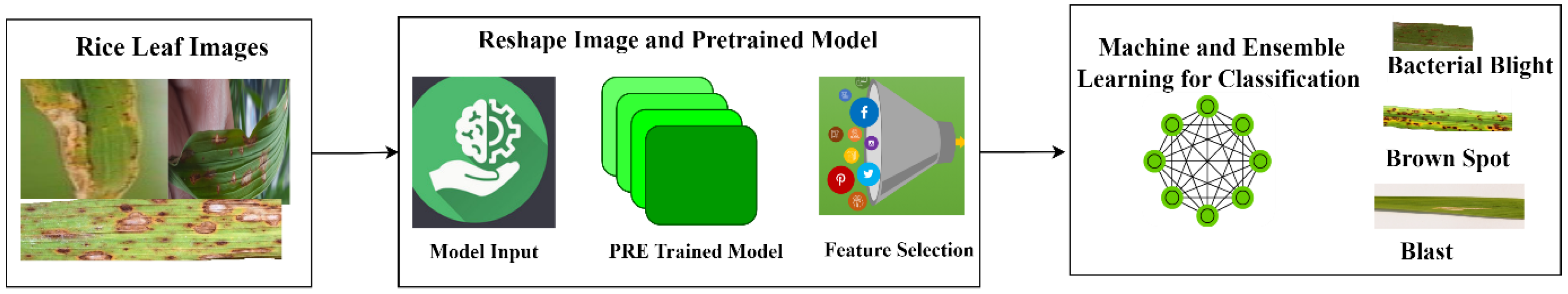
- Implementation of the pre-trained deep learning-based feature selection techniques on segmented images.
- Implementation analysis of machine and ensemble learning classification techniques using pre-trained deep learning models based on selected features.
- The experimental results show the effectiveness of the proposed procedure in comparison to existing techniques with high parameters for the classification of rice leaf diseases.
2. Materials and Methods
| Algorithm 1: Proposed Algorithm for Pre-trained Deep Neural Network-Based Features Selection Supported Machine Learning for Rice Leaf Disease Classification |
| Input: Infected rice leaf images ((Xi, Yi)…… (Xm, Ym)) Output: Class of rice leaf disease |
|
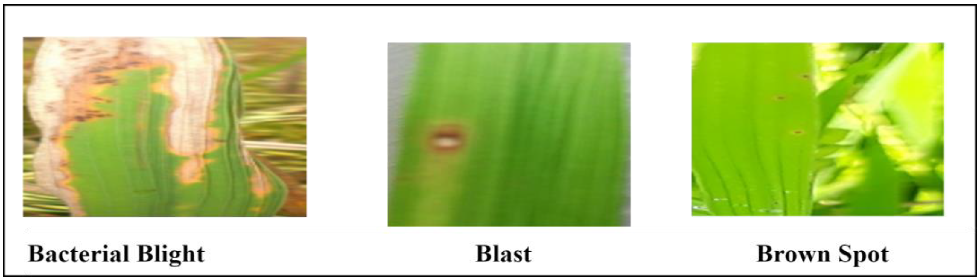
2.1. Data Acquisition and Pre-Processing
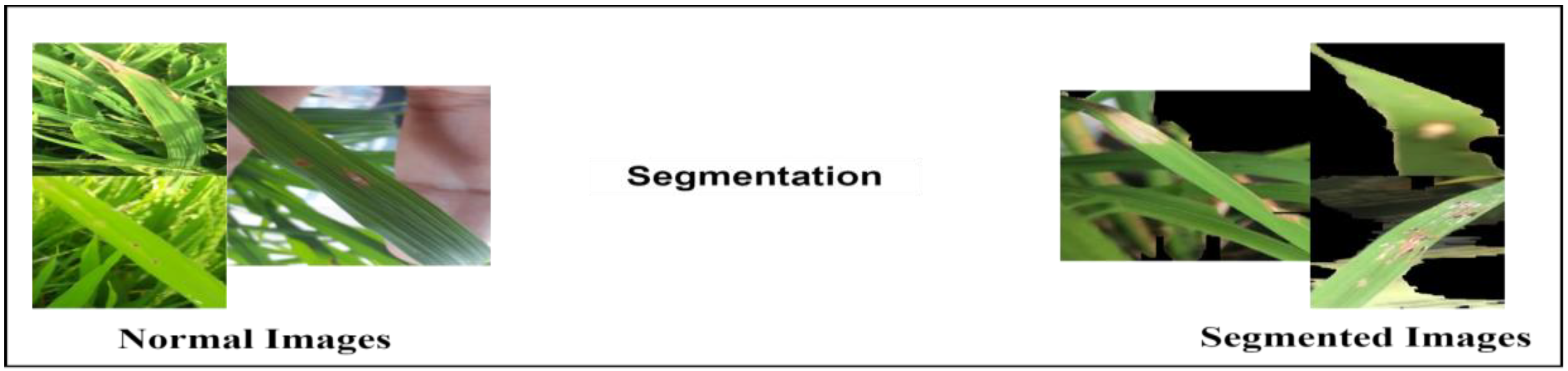
2.2. Segmentation
- (1)
- It can increase the quality of the image and reduce background noise in the lesion image, which will increase recognition accuracy.
- (2)
- It can decrease the volume of data, which will shorten the program’s execution time. To shorten the program’s runtime and increase the program’s recognition effectiveness.
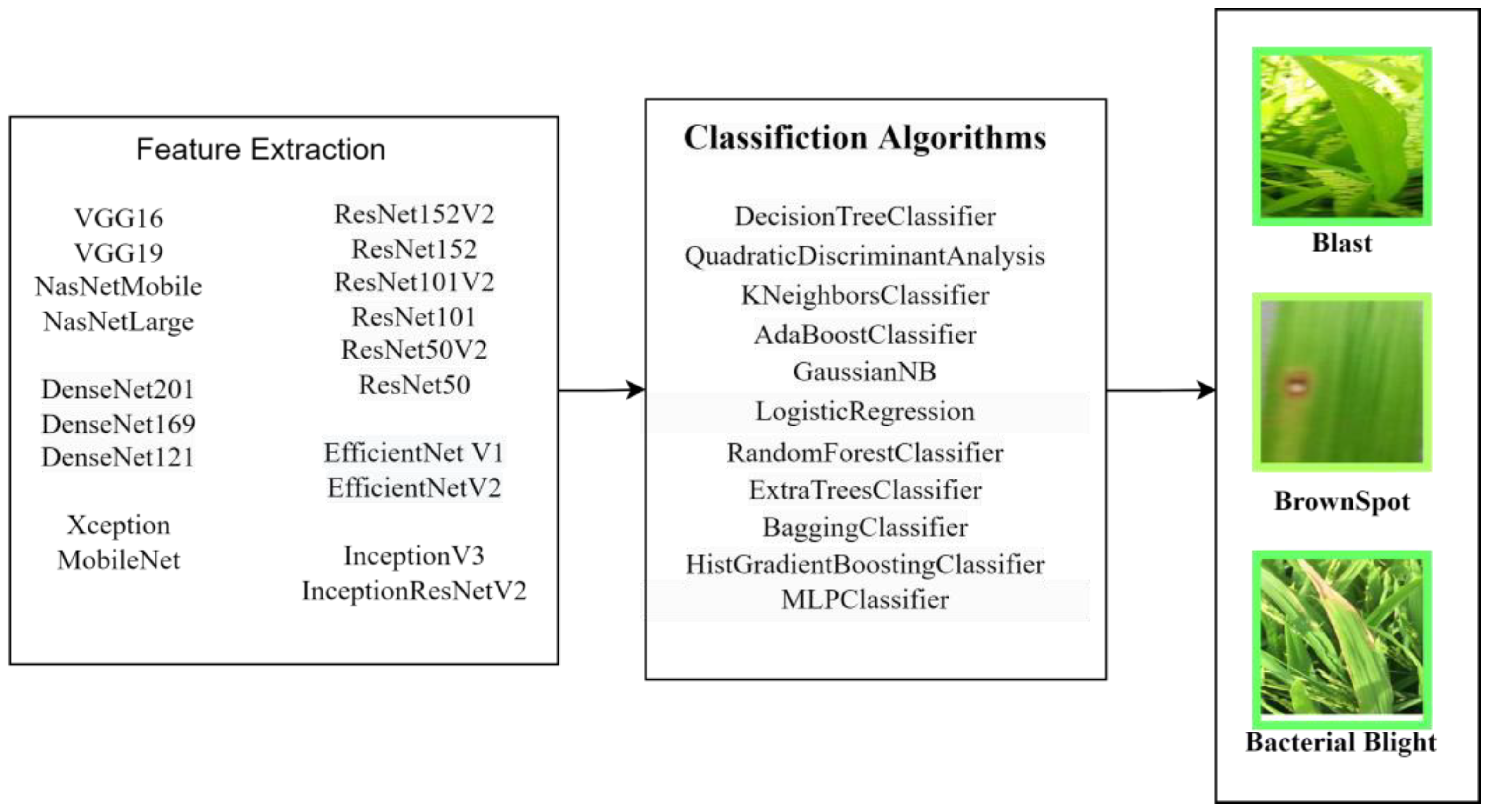
2.3. Feature Extraction Using Pre-Trained Models
2.4. Classification
2.5. Experimental Setup and Evaluation Metrics
3. Results
3.1. Analysis of Normal Data
3.2. Analysis on Segmented Data
3.3. Comparative Discussion
4. Conclusions
Author Contributions
Funding
Institutional Review Board Statement
Data Availability Statement
Acknowledgments
Conflicts of Interest
Abbreviation
| Abbreviation | Definition | Abbreviation | Definition |
| ML | Machine Learning | GNB | Gaussian Naïve Bayes |
| DL | Deep Learning | K-NN | K-Nearest Neighbour |
| DCNN | Deep CNN | LR | Logistic Regression |
| FS | False Smut | SVM | Support Vector Machine |
| BS | Brown Spot | DT | Decision Tree |
| SB | Sheath Blight | RF | Random factor |
| SB | Stem Borer | QDA | Quadratic Discriminant Analysis |
| LS | Leaf Smut | AB | Ada-boost |
| SR | Sheath Rot | ET | Extra Tree |
| FS | False Smut | HGB | Histogram Gradient boosting |
| BB | Bacterial Blight | GB | Gradient Boosting |
| MLP | Multi-Layer Preceptron | FN | False Negative |
| TP | True Positive | MC | Matthews Coefficient |
| TN | True Negative | KP | Kappa Statistics |
| FP | False Positive | YOLO | You only look once |
References
- Stanley, M. Food Staple. Available online: https://education.nationalgeographic.org/resource/food-staple (accessed on 26 December 2022).
- Kodama, T.; Hata, Y. Development of Classification System of Rice Disease Using Artificial Intelligence. In Proceedings of the 2018 IEEE International Conference on Systems, Man, and Cybernetics (SMC), Bari, Italy, 6–9 October 2019; pp. 3699–3702. [Google Scholar] [CrossRef]
- Chen, J.; Zhang, D.; Zeb, A.; Nanehkaran, Y.A. Identification of Rice Plant Diseases Using Lightweight Attention Networks. Expert Syst. Appl. 2021, 169, 114514. [Google Scholar] [CrossRef]
- Wani, J.A.; Sharma, S.; Muzamil, M.; Ahmed, S.; Sharma, S.; Singh, S. Machine Learning and Deep Learning Based Computational Techniques in Automatic Agricultural Diseases Detection: Methodologies, Applications, and Challenges. In Archives of Computational Methods in Engineering; Springer: Amsterdam, The Netherlands, 2022; Volume 29, pp. 641–677. ISBN 0123456789. [Google Scholar]
- Krishnamoorthy, N.; Prasad, L.N.; Kumar, C.P.; Subedi, B.; Abraha, H.B.; Sathishkumar, V.E. Rice Leaf Diseases Prediction Using Deep Neural Networks with Transfer Learning. Environ. Res. 2021, 198, 111275. [Google Scholar] [CrossRef]
- Prajapati, H.B.; Shah, J.P.; Dabhi, V.K. Detection and Classification of Rice Plant Diseases. Intell. Decis. Technol. 2017, 11, 357–373. [Google Scholar] [CrossRef]
- Gunawan, P.A.; Kencana, E.N.; Sari, K. Classification of Rice Leaf Diseases Using Artificial Neural Network. J. Phys. Conf. Ser. 2021, 1722, 012013. [Google Scholar] [CrossRef]
- Narmadha, R.P.; Arulvadivu, G. Detection and Measurement of Paddy Leaf Disease Symptoms Using Image Processing. In Proceedings of the 2017 International Conference on Computer Communication and Informatics (ICCCI), Tamilnadu, India, 5–7 January 2017; pp. 5–8. [Google Scholar] [CrossRef]
- Liu, L.W.; Hsieh, S.H.; Lin, S.J.; Wang, Y.M.; Lin, W.S. Rice Blast (Magnaporthe Oryzae) Occurrence Prediction and the Key Factor Sensitivity Analysis by Machine Learning. Agronomy 2021, 11, 771. [Google Scholar] [CrossRef]
- Sharma, T.; Kaur, P.; Chahal, J.; Sharma, H. Classification of Rice Leaf Diseases Based on the Deep Convolutional Neural Network Architectures: Review. In Proceedings of the AIP Conference Proceedings, Himachal Pradesh, India, 2–3 July 2022; Volume 2451. [Google Scholar]
- Maniyath, S.R.; Vinod, P.V.; Niveditha, M.; Pooja, R.; Prasad Bhat, N.; Shashank, N.; Hebbar, R. Plant Disease Detection Using Machine Learning. In Proceedings of the 2018 International Conference on Design Innovations for 3Cs Compute Communicate Control (ICDI3C), Bangalore, India, 25–28 April 2018; pp. 41–45. [Google Scholar] [CrossRef]
- Bari, B.S.; Islam, M.N.; Rashid, M.; Hasan, M.J.; Razman, M.A.M.; Musa, R.M.; Nasir, A.F.A.; Majeed, A.P.P.A. A Real-Time Approach of Diagnosing Rice Leaf Disease Using Deep Learning-Based Faster R-CNN Framework. PeerJ Comput. Sci. 2021, 7, e432. [Google Scholar] [CrossRef] [PubMed]
- Daniya, T.; Vigneshwari, S. Deep Neural Network for Disease Detection in Rice Plant Using the Texture and Deep Features. Comput. J. 2022, 65, 1812–1825. [Google Scholar] [CrossRef]
- Sethy, P.K.; Barpanda, N.K.; Rath, A.K.; Behera, S.K. Deep Feature Based Rice Leaf Disease Identification Using Support Vector Machine. Comput. Electron. Agric. 2020, 175, 105527. [Google Scholar] [CrossRef]
- Rautaray, S.S.; Pandey, M.; Gourisaria, M.K.; Sharma, R.; Das, S. Paddy Crop Disease Prediction—A Transfer Learning Technique. Int. J. Recent Technol. Eng. 2020, 8, 1490–1495. [Google Scholar] [CrossRef]
- Jadhav, A.A.J.B.D. Monitoring and Controlling Rice Diseases Using Image Processing Techniques. In Proceedings of the International Conference on Computing, Analytics and Security Trends (CAST), Pune, India, 19–21 December 2016; pp. 471–476. [Google Scholar]
- Sharma, V.; Mir, A.A.; Sarwr, D.A. Detection of Rice Disease Using Bayes’ Classifier and Minimum Distance Classifier. J. Multimed. Inf. Syst. 2020, 7, 17–24. [Google Scholar] [CrossRef]
- Lu, Y.; Yi, S.; Zeng, N.; Liu, Y.; Zhang, Y. Identification of Rice Diseases Using Deep Convolutional Neural Networks. Neurocomputing 2017, 267, 378–384. [Google Scholar] [CrossRef]
- Jiang, F.; Lu, Y.; Chen, Y.; Cai, D.; Li, G. Image Recognition of Four Rice Leaf Diseases Based on Deep Learning and Support Vector Machine. Comput. Electron. Agric. 2020, 179, 105824. [Google Scholar] [CrossRef]
- He, Y.; Zhou, Z.; Tian, L.; Liu, Y.; Luo, X. Brown Rice Planthopper (Nilaparvata Lugens Stal) Detection Based on Deep Learning. Precis. Agric. 2020, 21, 1385–1402. [Google Scholar] [CrossRef]
- Azim, M.A.; Islam, M.K.; Rahman, M.M.; Jahan, F. An Effective Feature Extraction Method for Rice Leaf Disease Classification. Telkomnika (Telecommun. Comput. Electron. Control) 2021, 19, 463–470. [Google Scholar] [CrossRef]
- Suresha, M.; Shreekanth, K.N.; Thirumalesh, B.V. Recognition of Diseases in Paddy Leaves Using Knn Classifier. In Proceedings of the 2nd International Conference for Convergence in Technology, I2CT, Mumbai, India, 7–9 April 2017; pp. 663–666. [Google Scholar]
- Sardogan, M.; Tuncer, A.; Ozen, Y. Plant Leaf Disease Detection and Classification Based on CNN with LVQ Algorithm. In Proceedings of the UBMK—3rd International Conference on Computer Science and Engineering, Sarajevo, Bosnia and Herzegovina, 20–23 September 2018; pp. 382–385. [Google Scholar]
- Liang, W.-J.; Zhang, H.; Zhang, G.F.; Cao, H.-X. Rice Blast Disease Recognition Using a Deep Convolutional Neural Network. Sci. Rep. 2019, 9, 2869. [Google Scholar] [CrossRef] [PubMed]
- Nidhis, A.D.; Pardhu, C.N.V.; Reddy, K.C.; Deepa, K. Cluster Based Paddy Leaf Disease Detection, Classification and Diagnosis in Crop Health Monitoring Unit. In Lecture Notes in Computational Vision and Biomechanics; Springer International Publishing: New York, NY, USA, 2019; Volume 31, pp. 281–291. ISBN 9783030040611. [Google Scholar]
- Anami, B.S.; Malvade, N.N.; Palaiah, S. Deep Learning Approach for Recognition and Classification of Yield Affecting Paddy Crop Stresses Using Field Images. Artif. Intell. Agric. 2020, 4, 12–20. [Google Scholar] [CrossRef]
- Ghosal, S.; Sarkar, K. Rice Leaf Diseases Classification Using CNN with Transfer Learning. In Proceedings of the IEEE Calcutta Conference, CALCON–Proceedings, Kolkata, India, 28–29 February 2020; pp. 230–236. [Google Scholar]
- Li, D.; Wang, R.; Xie, C.; Liu, L.; Zhang, J.; Li, R.; Wang, F.; Zhou, M.; Liu, W. A Recognition Method for Rice Plant Diseases and Pests Video Detection Based on Deep Convolutional Neural Network. Sensors 2020, 20, 578. [Google Scholar] [CrossRef] [PubMed]
- Matin, M.M.H.; Khatun, A.; Moazzam, M.G.; Uddin, M.S. An Efficient Disease Detection Technique of Rice Leaf Using AlexNet. J. Comput. Commun. 2020, 8, 49–57. [Google Scholar] [CrossRef]
- Temniranrat, P.; Kiratiratanapruk, K.; Kitvimonrat, A.; Sinthupinyo, W.; Patarapuwadol, S. A System for Automatic Rice Disease Detection from Rice Paddy Images Serviced via a Chatbot. Comput. Electron. Agric. 2021, 185, 106156. [Google Scholar] [CrossRef]
- Francisco, A.K.G. Rice Disease Data Set. Available online: https://github.com/aldrin233/RiceDiseases-DataSet (accessed on 12 October 2022).
- Sethy, P.K.; Barpanda, N.K.; Rath, A.K.; Behera, S.K. Image Processing Techniques for Diagnosing Rice Plant Disease: A Survey. Procedia Comput. Sci. 2020, 167, 516–530. [Google Scholar] [CrossRef]
- Krichen, M.; Mihoub, A.; Alzahrani, M.Y.; Adoni, W.Y.H.; Nahhal, T. Are Formal Methods Applicable To Machine Learning And Artificial Intelligence? In Proceedings of the International Conference of Smart Systems and Emerging Technologies (SMARTTECH), Riyadh, Saudi Arabia, 9–11 May 2022; pp. 48–53. [Google Scholar]
- Seshia, S.A.; Sadigh, D.; Sastry, S.S. Toward Verified Artificial Intelligence. Commun. ACM 2022, 65, 46–55. [Google Scholar] [CrossRef]
- Anantrasirichai, N.; Hannuna, S.; Canagarajah, N. Automatic Leaf Extraction from Outdoor Images. arXiv 2017, arXiv:1709.06437. [Google Scholar] [CrossRef]
- Watershed Alogithm and Application. Available online: https://www.aegissofttech.com/articles/watershed-algorithm-and-limitations.html (accessed on 25 December 2022).
- Dara, S.; Tumma, P. Feature Extraction by Using Deep Learning: A Survey. In Proceedings of the 2nd International Conference on Electronics, Communication and Aerospace Technology, ICECA 2018, Coimbatore, India, 29–31 March 2018; pp. 1795–1801. [Google Scholar]
- Rallapalli, S.M.; Saleem Durai, M.A. A Contemporary Approach for Disease Identification in Rice Leaf. Int. J. Syst. Assur. Eng. Manag. 2021, 1–11. [Google Scholar] [CrossRef]
- Sengupta, S.; Dutta, A.; Abdelmohsen, S.A.M.; Alyousef, H.A.; Rahimi-Gorji, M. Development of a Rice Plant Disease Classification Model in Big Data Environment. Bioengineering 2022, 9, 758. [Google Scholar] [CrossRef] [PubMed]
- Chen, J.; Chen, J.; Zhang, D.; Sun, Y.; Nanehkaran, Y.A. Using Deep Transfer Learning for Image-Based Plant Disease Identification. Comput. Electron. Agric. 2020, 173, 105393. [Google Scholar] [CrossRef]
- Kaur, A.; Guleria, K.; Trivedi, N. A Deep Learning Based Model for Rice Leaf Disease Detection. In Proceedings of the 10th International Conference on Reliability, Infocom Technologies and Optimization (Trends and Future Directions) (ICRITO), Noida, India, 13–14 October 2022; pp. 1–5. [Google Scholar]


| Disease | Stage | Symptoms | Important Season | Factors for Infection |
|---|---|---|---|---|
| Blast | In growing stage | Green-grey spot with dark green outline and more difficult to detect with grey centre and green outline | Rain shower and cooled temperature | High humidity and nitrogen level |
| Sheath Blight | At tillering | Greenish grey irregular spot between water and leaf blade | Rainy season | High temperature and humidity with high level of nitrogen |
| False Smut | At flowering to maturity | Follicles are in orange and at maturity turn greenish yellow or black | In periodic rain fall | Extreme nitrogen and high humidity |
| Brown Spot | Flowering to maturity | Brown to purple-brown oval spot on leaves | Periodic rain | High humidity, soil deficiency and high temperature |
| Bacterial Blight | Tillering to heading | Tan-greyish to white | In wet | High temperature and humidity |
| References | ML/DL Technique | Disease Type | Data Set Size (Images) | Improved Technique | Performance Measure/Score | Limitation |
|---|---|---|---|---|---|---|
| [22] | K-NN classifier with global threshold | Blast, BS | 330 | Segmentation | Accuracy = 0.76 | Lower accuracy |
| [18] | Deep CNN | Blast, FS, BS, SB | 500 | None | Accuracy mean = 0.95 | Time consuming because deep learning architectures contained several layers |
| [23] | LVQ with CNN | BS | 500 | None | Accuracy = 0.86 | Only one class is used |
| [24] | DCNN | Rice blast | 5808 | None | Mean Accuracy = 0.89 AUC = 0.95 | Only one rice disease discussed |
| [25] | Image Processing | BB, BS, blast | - | Segmentation | Accuracy = 0.91 | Back propagation method was not discussed |
| [26] | DCNN VGG-16 | BB, FS | 6000 | None | Accuracy 0.95 | Feature extraction technique was not accurate |
| [21] | Extreme Gradient Boosting | BB, LS, BS | 120 | Segmentation | Accuracy = 0.86 F1-Score = 0.87 | Less data set size |
| [27] | CNN with Transfer Learning (VGG 16) | Blight BS, LB | 1649 | Augmentation | Accuracy = 0.92 | Augmentation approach is not appropriate |
| [20] | RCNN | Brown rice plant hooper | 4600 | None | Accuracy = 0.94 Recall rate = 0.88 | Feature extraction technique was not appropriate |
| [28] | VGG16, ResNet50, ResNet101, and YOLOv3 | SB, BS | 5320 | None | Mean F1-score = 0.74, Recall rate = 0.77 Precision = 0.74 | Performance parameters are low |
| [29] | AlexNet Neural Network | BS, BB, LS | 900 | Augmentation | Accuracy = 0.9 | Augmentation technique was appropriate |
| [7] | ANN | BS, LS | 96 | Segmentation | Accuracy = 0.79 | Less data set |
| [9] | Probabilistic Neural Network (PNN) | Rice blast | 1800 | None | Accuracy = 0.91 F1-Score = 0.92 | Only one rice leaf disease was discussed |
| [5] | CNN and InceptionResNeV2 | Blast, BB, BS | 5200 | Augmentation | Accuracy = 0.95 | Feature extraction technique was not appropriate |
| [30] | Neural Network with YOLOv3 | Blast, BS Streak | 6538 | None | TPR = 0.78 | Performance parameters are not enough |
| Disease Name | No. of Images | Images for Training (80%) | Images for Validation (20%) |
|---|---|---|---|
| Bacterial leaf Blight | 192 | 154 | 38 |
| Brown Spot | 200 | 160 | 40 |
| Blast | 159 | 127 | 32 |
| Total | 551 | 441 | 110 |
| Model | Input Shape | Selected Features Size | Number of Parameters | Memory (in Bytes) | Feature Layer |
|---|---|---|---|---|---|
| Xception | (229, 229, 3) | 2048 | 20,861,480 | 272,784,948 | Global Average Pooling 2D |
| VGG16 | (224, 224, 3) | 4096 | 134,260,544 | 195,307,328 | Dense |
| VGG19 | (224, 224, 3) | 4096 | 139,570,240 | 205,835,328 | Dense |
| ResNet50 | (224, 224, 3) | 2048 | 23,587,712 | 172,064,560 | Global Average Pooling 2D |
| ResNet50V2 | (224, 224, 3) | 2048 | 23,564,800 | 149,085,616 | Global Average Pooling 2D |
| ResNet101 | (224, 224, 3) | 2048 | 42,658,176 | 266,198,320 | Global Average Pooling 2D |
| ResNet101V2 | (224, 224, 3) | 2048 | 42,626,560 | 247,667,120 | Global Average Pooling 2D |
| ResNet152 | (224, 224, 3) | 2048 | 58,370,944 | 374,636,336 | Global Average Pooling 2D |
| ResNet152V2 | (224, 224, 3) | 2048 | 58,331,648 | 361,348,528 | Global Average Pooling 2D |
| InceptionV3 | (229, 229, 3) | 2048 | 21,802,784 | 152,016,332 | Global Average Pooling 2D |
| InceptionResNetV2 | (229, 229, 3) | 1536 | 54,336,736 | 379,140,364 | Global Average Pooling 2D |
| MobileNet | (224, 224, 3) | 1000 | 4,253,864 | 71,638,760 | Reshape |
| DenseNet121 | (224, 224, 3) | 1024 | 7,037,504 | 206,739,952 | Global Average Pooling 2D |
| DenseNet169 | (224, 224, 3) | 1664 | 12,642,880 | 253,015,536 | Global Average Pooling 2D |
| DenseNet201 | (224, 224, 3) | 1920 | 18,321,984 | 327,486,960 | Global Average Pooling 2D |
| NASNetMobile | (224, 224, 3) | 1056 | 4,269,716 | 115,028,536 | Global Average Pooling 2D |
| NASNetLarge | (331, 331, 3) | 4032 | 84,916,818 | 1,247,153,502 | Global Average Pooling 2D |
| EfficientNet B0 | 224, 224, 3 | 1280 | 4,049,571 | 105,116,063 | Dropout |
| EfficientNet B1 | 240, 240, 3 | 1280 | 6,575,239 | 167,863,763 | Dropout |
| EfficientNet B2 | 260, 260, 3 | 1408 | 7,768,569 | 212,211,693 | Dropout |
| EfficientNet B3 | 300, 300, 3 | 1536 | 10,783,535 | 361,891,419 | Dropout |
| EfficientNet B4 | 380, 380, 3 | 1792 | 17,673,823 | 739,756,747 | Dropout |
| EfficientNet B5 | 456, 456, 3 | 2048 | 28,513,527 | 1,464,166,467 | Dropout |
| EfficientNet B6 | 528, 528, 3 | 2304 | 40,960,143 | 2,466,985,915 | Dropout |
| EfficientNet B7 | 600, 600, 3 | 2560 | 64,097,687 | 4,252,866,467 | Dropout |
| EfficientNetV2B0 | 224, 224, 3 | 1280 | 5,919,312 | 70,588,560 | Dropout |
| EfficientNetV2B1 | 240, 240, 3 | 1280 | 6,931,124 | 107,709,828 | Dropout |
| EfficientNetV2B2 | 260, 260, 3 | 1408 | 8,769,374 | 143,981,142 | Dropout |
| EfficientNetV2B3 | 300, 300, 3 | 1536 | 12,930,622 | 228,894,934 | Dropout |
| EfficientNetV2S | 384, 384, 3 | 1280 | 20,331,360 | 512,960,320 | Dropout |
| EfficientNetV2M | 480, 480, 3 | 1280 | 53,150,388 | 1,301,769,700 | Dropout |
| EfficientNetV2L | 480, 480, 3 | 1280 | 117,746,848 | 2,317,398,688 | Dropout |
| Metrics | Definition | Formula |
|---|---|---|
| Accuracy | Comparison between actual and predicted value | Accuracy = (TP + TN)/TP + FP + TN + FN) |
| Precision | Actual corrected positive prediction | Precision = TP/(TP + FP) |
| Recall rate | Actual positive incorrected prediction | Recall = TP/(TP + FN) |
| F1-score | Single value for both precision and recall rate | F1-Score = 2TP/(2TP + FP + FN) |
| MC (Matthews Coefficient) | Used to measure of the quality of binary and multiclass classification. | MC = (TP × TN)(FP × FN)/ |
| KP (Kappa Statistics) | Used to measure the inter-rater reliability for categorical items. | K = (po − pe)/(1 − pe) |
| Classifiers/ Pre-Trained Model | DT | QDA | KNN | AB | GNB | LR | RF | ET | HGB | MLP |
|---|---|---|---|---|---|---|---|---|---|---|
| Xception | 0.7 | 0.35 | 0.63 | 0.66 | 0.66 | 0.65 | 0.79 | 0.8 | 0.86 | 0.69 |
| VGG19 | 0.67 | 0.39 | 0.67 | 0.72 | 0.59 | 0.64 | 0.82 | 0.83 | 0.83 | 0.79 |
| VGG16 | 0.61 | 0.36 | 0.64 | 0.66 | 0.69 | 0.56 | 0.82 | 0.81 | 0.78 | 0.73 |
| ResNet152V2 | 0.63 | 0.38 | 0.56 | 0.66 | 0.57 | 0.54 | 0.76 | 0.78 | 0.8 | 0.65 |
| ResNet152 | 0.74 | 0.48 | 0.72 | 0.77 | 0.56 | 0.66 | 0.83 | 0.83 | 0.84 | 0.7 |
| ResNet101V2 | 0.56 | 0.41 | 0.56 | 0.67 | 0.63 | 0.59 | 0.74 | 0.71 | 0.79 | 0.7 |
| ResNet101 | 0.71 | 0.44 | 0.68 | 0.71 | 0.62 | 0.7 | 0.84 | 0.81 | 0.81 | 0.77 |
| ResNet50V2 | 0.54 | 0.38 | 0.53 | 0.71 | 0.65 | 0.53 | 0.76 | 0.78 | 0.73 | 0.66 |
| ResNet50 | 0.72 | 0.47 | 0.7 | 0.71 | 0.6 | 0.65 | 0.84 | 0.81 | 0.8 | 0.73 |
| NASNetMobile | 0.61 | 0.45 | 0.62 | 0.67 | 0.51 | 0.57 | 0.77 | 0.77 | 0.78 | 0.66 |
| NASNetLarge | 0.7 | 0.44 | 0.62 | 0.66 | 0.36 | 0.73 | 0.81 | 0.78 | 0.8 | 0.72 |
| MobileNet | 0.61 | 0.4 | 0.55 | 0.61 | 0.61 | 0.69 | 0.79 | 0.81 | 0.8 | 0.7 |
| InceptionV3 | 0.65 | 0.39 | 0.64 | 0.66 | 0.77 | 0.61 | 0.79 | 0.83 | 0.77 | 0.76 |
| InceptionResNetV2 | 0.64 | 0.48 | 0.68 | 0.65 | 0.79 | 0.67 | 0.79 | 0.82 | 0.8 | 0.72 |
| EfficientNetV2S | 0.72 | 0.4 | 0.76 | 0.69 | 0.71 | 0.69 | 0.91 | 0.89 | 0.89 | 0.73 |
| EfficientNetV2M | 0.66 | 0.38 | 0.47 | 0.71 | 0.67 | 0.57 | 0.77 | 0.79 | 0.79 | 0.66 |
| EfficientNetV2L | 0.66 | 0.38 | 0.66 | 0.56 | 0.78 | 0.64 | 0.82 | 0.87 | 0.87 | 0.74 |
| EfficientNetV2B3 | 0.68 | 0.43 | 0.72 | 0.81 | 0.78 | 0.76 | 0.85 | 0.9 | 0.89 | 0.85 |
| EfficientNetV2B2 | 0.69 | 0.39 | 0.61 | 0.69 | 0.61 | 0.56 | 0.8 | 0.78 | 0.81 | 0.66 |
| EfficientNetV2B1 | 0.71 | 0.41 | 0.61 | 0.73 | 0.6 | 0.63 | 0.78 | 0.8 | 0.82 | 0.69 |
| EfficientNetV2B0 | 0.63 | 0.33 | 0.63 | 0.67 | 0.6 | 0.57 | 0.76 | 0.76 | 0.74 | 0.77 |
| EfficientNetB7 | 0.83 | 0.46 | 0.65 | 0.73 | 0.79 | 0.71 | 0.86 | 0.86 | 0.83 | 0.74 |
| EfficientNetB6 | 0.71 | 0.43 | 0.72 | 0.63 | 0.67 | 0.6 | 0.9 | 0.86 | 0.86 | 0.74 |
| EfficientNetB5 | 0.64 | 0.44 | 0.69 | 0.79 | 0.71 | 0.63 | 0.85 | 0.88 | 0.83 | 0.74 |
| EfficientNetB4 | 0.69 | 0.46 | 0.76 | 0.78 | 0.71 | 0.65 | 0.81 | 0.83 | 0.85 | 0.74 |
| EfficientNetB3 | 0.76 | 0.4 | 0.7 | 0.81 | 0.87 | 0.69 | 0.89 | 0.91 | 0.91 | 0.86 |
| EfficientNetB2 | 0.74 | 0.5 | 0.61 | 0.65 | 0.67 | 0.66 | 0.77 | 0.82 | 0.78 | 0.71 |
| EfficientNetB1 | 0.68 | 0.4 | 0.67 | 0.72 | 0.63 | 0.69 | 0.8 | 0.83 | 0.8 | 0.71 |
| EfficientNetB0 | 0.65 | 0.36 | 0.7 | 0.73 | 0.63 | 0.57 | 0.8 | 0.83 | 0.82 | 0.71 |
| DenseNet201 | 0.6 | 0.34 | 0.56 | 0.73 | 0.64 | 0.63 | 0.79 | 0.77 | 0.81 | 0.65 |
| DenseNet169 | 0.59 | 0.36 | 0.64 | 0.7 | 0.53 | 0.66 | 0.81 | 0.78 | 0.77 | 0.67 |
| DenseNet121 | 0.72 | 0.4 | 0.71 | 0.74 | 0.4 | 0.62 | 0.79 | 0.81 | 0.83 | 0.72 |
| Classifiers/ Pre-Trained Model | DT | QDA | KNN | AB | GNB | LR | RF | ET | HGB | MLP |
|---|---|---|---|---|---|---|---|---|---|---|
| Xception | 0.67 | 0.23 | 0.52 | 0.69 | 0.64 | 0.44 | 0.72 | 0.77 | 0.83 | 0.64 |
| VGG19 | 0.62 | 0.23 | 0.6 | 0.69 | 0.59 | 0.62 | 0.77 | 0.78 | 0.79 | 0.74 |
| VGG16 | 0.55 | 0.21 | 0.62 | 0.67 | 0.67 | 0.39 | 0.77 | 0.75 | 0.73 | 0.67 |
| ResNet152V2 | 0.59 | 0.23 | 0.49 | 0.59 | 0.55 | 0.36 | 0.66 | 0.7 | 0.76 | 0.61 |
| ResNet152 | 0.69 | 0.3 | 0.67 | 0.72 | 0.61 | 0.61 | 0.78 | 0.78 | 0.79 | 0.67 |
| ResNet101V2 | 0.51 | 0.25 | 0.5 | 0.63 | 0.62 | 0.5 | 0.67 | 0.62 | 0.74 | 0.63 |
| ResNet101 | 0.66 | 0.3 | 0.65 | 0.66 | 0.71 | 0.47 | 0.79 | 0.75 | 0.76 | 0.7 |
| ResNet50V2 | 0.48 | 0.24 | 0.45 | 0.66 | 0.69 | 0.54 | 0.69 | 0.73 | 0.67 | 0.63 |
| ResNet50 | 0.67 | 0.28 | 0.57 | 0.67 | 0.62 | 0.58 | 0.79 | 0.75 | 0.74 | 0.7 |
| NASNetMobile | 0.57 | 0.29 | 0.57 | 0.63 | 0.44 | 0.53 | 0.71 | 0.71 | 0.72 | 0.61 |
| NASNetLarge | 0.66 | 0.23 | 0.57 | 0.64 | 0.6 | 0.5 | 0.77 | 0.74 | 0.78 | 0.6 |
| MobileNet | 0.59 | 0.15 | 0.52 | 0.56 | 0.69 | 0.64 | 0.75 | 0.74 | 0.76 | 0.65 |
| InceptionV3 | 0.62 | 0.22 | 0.53 | 0.69 | 0.73 | 0.43 | 0.75 | 0.78 | 0.71 | 0.71 |
| InceptionResNetV2 | 0.6 | 0.28 | 0.63 | 0.65 | 0.76 | 0.47 | 0.75 | 0.79 | 0.76 | 0.67 |
| EfficientNetV2S | 0.67 | 0.24 | 0.7 | 0.63 | 0.7 | 0.62 | 0.89 | 0.85 | 0.85 | 0.68 |
| EfficientNetV2M | 0.61 | 0.24 | 0.4 | 0.66 | 0.63 | 0.58 | 0.68 | 0.72 | 0.7 | 0.55 |
| EfficientNetV2L | 0.59 | 0.21 | 0.58 | 0.6 | 0.73 | 0.66 | 0.77 | 0.85 | 0.85 | 0.67 |
| EfficientNetV2B3 | 0.62 | 0.26 | 0.66 | 0.75 | 0.72 | 0.84 | 0.81 | 0.91 | 0.92 | 0.81 |
| EfficientNetV2B2 | 0.66 | 0.27 | 0.56 | 0.67 | 0.62 | 0.48 | 0.74 | 0.72 | 0.75 | 0.62 |
| EfficientNetV2B1 | 0.67 | 0.21 | 0.57 | 0.71 | 0.53 | 0.46 | 0.73 | 0.76 | 0.78 | 0.66 |
| EfficientNetV2B0 | 0.59 | 0.22 | 0.59 | 0.63 | 0.68 | 0.62 | 0.71 | 0.7 | 0.68 | 0.72 |
| EfficientNetB7 | 0.79 | 0.28 | 0.56 | 0.69 | 0.75 | 0.65 | 0.88 | 0.9 | 0.79 | 0.7 |
| EfficientNetB6 | 0.71 | 0.27 | 0.68 | 0.66 | 0.7 | 0.43 | 0.88 | 0.82 | 0.82 | 0.69 |
| EfficientNetB5 | 0.61 | 0.28 | 0.66 | 0.74 | 0.69 | 0.42 | 0.82 | 0.86 | 0.81 | 0.71 |
| EfficientNetB4 | 0.65 | 0.28 | 0.67 | 0.74 | 0.7 | 0.46 | 0.78 | 0.79 | 0.8 | 0.7 |
| EfficientNetB3 | 0.72 | 0.24 | 0.66 | 0.78 | 0.84 | 0.72 | 0.89 | 0.91 | 0.9 | 0.84 |
| EfficientNetB2 | 0.67 | 0.32 | 0.57 | 0.65 | 0.64 | 0.63 | 0.7 | 0.76 | 0.74 | 0.66 |
| EfficientNetB1 | 0.64 | 0.25 | 0.61 | 0.72 | 0.66 | 0.62 | 0.75 | 0.78 | 0.77 | 0.66 |
| EfficientNetB0 | 0.63 | 0.18 | 0.63 | 0.68 | 0.63 | 0.53 | 0.74 | 0.76 | 0.76 | 0.65 |
| DenseNet201 | 0.55 | 0.19 | 0.53 | 0.71 | 0.63 | 0.43 | 0.72 | 0.7 | 0.75 | 0.61 |
| DenseNet169 | 0.56 | 0.2 | 0.57 | 0.66 | 0.58 | 0.55 | 0.75 | 0.71 | 0.71 | 0.62 |
| DenseNet121 | 0.69 | 0.26 | 0.69 | 0.71 | 0.55 | 0.61 | 0.73 | 0.76 | 0.78 | 0.68 |
| Classifiers/ Pre-Trained Model | DT | QDA | KNN | AB | GNB | LR | RF | ET | HGB | MLP |
|---|---|---|---|---|---|---|---|---|---|---|
| Xception | 0.67 | 0.39 | 0.53 | 0.67 | 0.63 | 0.52 | 0.69 | 0.76 | 0.84 | 0.63 |
| VGG19 | 0.63 | 0.38 | 0.6 | 0.68 | 0.56 | 0.55 | 0.78 | 0.78 | 0.78 | 0.74 |
| VGG16 | 0.55 | 0.36 | 0.62 | 0.68 | 0.68 | 0.45 | 0.78 | 0.76 | 0.72 | 0.66 |
| ResNet152V2 | 0.47 | 0.41 | 0.45 | 0.66 | 0.66 | 0.48 | 0.68 | 0.72 | 0.66 | 0.64 |
| ResNet152 | 0.67 | 0.47 | 0.58 | 0.67 | 0.56 | 0.58 | 0.79 | 0.75 | 0.74 | 0.7 |
| ResNet101V2 | 0.58 | 0.39 | 0.49 | 0.59 | 0.49 | 0.43 | 0.66 | 0.7 | 0.74 | 0.61 |
| ResNet101 | 0.68 | 0.45 | 0.68 | 0.72 | 0.52 | 0.61 | 0.79 | 0.78 | 0.8 | 0.68 |
| ResNet50V2 | 0.51 | 0.41 | 0.5 | 0.61 | 0.57 | 0.49 | 0.66 | 0.62 | 0.71 | 0.62 |
| ResNet50 | 0.66 | 0.52 | 0.67 | 0.67 | 0.58 | 0.56 | 0.8 | 0.76 | 0.77 | 0.69 |
| NASNetMobile | 0.57 | 0.51 | 0.56 | 0.62 | 0.43 | 0.52 | 0.7 | 0.71 | 0.7 | 0.61 |
| NASNetLarge | 0.66 | 0.38 | 0.57 | 0.63 | 0.46 | 0.59 | 0.76 | 0.73 | 0.74 | 0.6 |
| MobileNet | 0.61 | 0.32 | 0.51 | 0.55 | 0.54 | 0.6 | 0.72 | 0.72 | 0.75 | 0.62 |
| InceptionV3 | 0.61 | 0.36 | 0.54 | 0.66 | 0.71 | 0.48 | 0.72 | 0.75 | 0.71 | 0.69 |
| InceptionResNetV2 | 0.59 | 0.48 | 0.63 | 0.63 | 0.76 | 0.54 | 0.76 | 0.77 | 0.74 | 0.67 |
| EfficientNetV2S | 0.68 | 0.38 | 0.71 | 0.61 | 0.72 | 0.62 | 0.87 | 0.84 | 0.84 | 0.69 |
| EfficientNetV2M | 0.62 | 0.39 | 0.4 | 0.65 | 0.62 | 0.48 | 0.68 | 0.71 | 0.68 | 0.55 |
| EfficientNetV2L | 0.59 | 0.35 | 0.58 | 0.59 | 0.73 | 0.52 | 0.74 | 0.8 | 0.85 | 0.66 |
| EfficientNetV2B3 | 0.62 | 0.43 | 0.65 | 0.76 | 0.72 | 0.62 | 0.78 | 0.85 | 0.86 | 0.79 |
| EfficientNetV2B2 | 0.68 | 0.47 | 0.56 | 0.67 | 0.58 | 0.49 | 0.73 | 0.71 | 0.74 | 0.6 |
| EfficientNetV2B1 | 0.68 | 0.35 | 0.57 | 0.73 | 0.5 | 0.5 | 0.72 | 0.76 | 0.77 | 0.61 |
| EfficientNetV2B0 | 0.57 | 0.35 | 0.59 | 0.63 | 0.64 | 0.56 | 0.71 | 0.69 | 0.68 | 0.73 |
| EfficientNetB7 | 0.79 | 0.45 | 0.56 | 0.69 | 0.72 | 0.58 | 0.83 | 0.8 | 0.78 | 0.67 |
| EfficientNetB6 | 0.73 | 0.43 | 0.67 | 0.66 | 0.67 | 0.47 | 0.86 | 0.83 | 0.84 | 0.68 |
| EfficientNetB5 | 0.6 | 0.48 | 0.68 | 0.74 | 0.69 | 0.5 | 0.82 | 0.84 | 0.78 | 0.71 |
| EfficientNetB4 | 0.64 | 0.45 | 0.67 | 0.75 | 0.71 | 0.52 | 0.8 | 0.81 | 0.81 | 0.71 |
| EfficientNetB3 | 0.73 | 0.39 | 0.65 | 0.8 | 0.85 | 0.59 | 0.87 | 0.89 | 0.89 | 0.84 |
| EfficientNetB2 | 0.67 | 0.5 | 0.57 | 0.63 | 0.65 | 0.61 | 0.69 | 0.77 | 0.75 | 0.66 |
| EfficientNetB1 | 0.63 | 0.42 | 0.6 | 0.73 | 0.64 | 0.62 | 0.75 | 0.78 | 0.79 | 0.66 |
| EfficientNetB0 | 0.64 | 0.31 | 0.61 | 0.69 | 0.61 | 0.49 | 0.74 | 0.75 | 0.74 | 0.63 |
| DenseNet201 | 0.55 | 0.32 | 0.52 | 0.71 | 0.58 | 0.5 | 0.72 | 0.7 | 0.76 | 0.61 |
| DenseNet169 | 0.56 | 0.31 | 0.57 | 0.65 | 0.56 | 0.55 | 0.75 | 0.7 | 0.7 | 0.62 |
| DenseNet121 | 0.7 | 0.45 | 0.68 | 0.71 | 0.46 | 0.58 | 0.73 | 0.76 | 0.79 | 0.69 |
| Classifiers/ Pre-Trained Model | DT | QDA | KNN | AB | GNB | LR | RF | ET | HGB | MLP |
|---|---|---|---|---|---|---|---|---|---|---|
| Xception | 0.67 | 0.28 | 0.52 | 0.64 | 0.62 | 0.47 | 0.7 | 0.77 | 0.83 | 0.63 |
| VGG19 | 0.62 | 0.29 | 0.6 | 0.68 | 0.55 | 0.54 | 0.78 | 0.78 | 0.78 | 0.74 |
| VGG16 | 0.55 | 0.27 | 0.62 | 0.64 | 0.66 | 0.4 | 0.78 | 0.76 | 0.73 | 0.66 |
| ResNet152V2 | 0.47 | 0.3 | 0.44 | 0.66 | 0.62 | 0.47 | 0.68 | 0.72 | 0.66 | 0.63 |
| ResNet152 | 0.66 | 0.35 | 0.55 | 0.66 | 0.53 | 0.58 | 0.79 | 0.75 | 0.74 | 0.69 |
| ResNet101V2 | 0.58 | 0.29 | 0.49 | 0.59 | 0.49 | 0.39 | 0.65 | 0.7 | 0.74 | 0.6 |
| ResNet101 | 0.68 | 0.35 | 0.67 | 0.72 | 0.47 | 0.61 | 0.79 | 0.78 | 0.79 | 0.66 |
| ResNet50V2 | 0.51 | 0.31 | 0.5 | 0.61 | 0.57 | 0.48 | 0.66 | 0.62 | 0.71 | 0.62 |
| ResNet50 | 0.66 | 0.36 | 0.65 | 0.66 | 0.57 | 0.51 | 0.79 | 0.75 | 0.76 | 0.69 |
| NASNetMobile | 0.57 | 0.36 | 0.55 | 0.62 | 0.42 | 0.52 | 0.71 | 0.71 | 0.7 | 0.61 |
| NASNetLarge | 0.66 | 0.28 | 0.57 | 0.62 | 0.37 | 0.54 | 0.76 | 0.73 | 0.75 | 0.59 |
| MobileNet | 0.59 | 0.21 | 0.51 | 0.54 | 0.54 | 0.61 | 0.73 | 0.73 | 0.75 | 0.63 |
| InceptionV3 | 0.6 | 0.27 | 0.53 | 0.64 | 0.72 | 0.44 | 0.73 | 0.76 | 0.71 | 0.7 |
| InceptionResNetV2 | 0.59 | 0.35 | 0.63 | 0.62 | 0.76 | 0.5 | 0.75 | 0.78 | 0.74 | 0.67 |
| EfficientNetV2S | 0.67 | 0.29 | 0.7 | 0.6 | 0.69 | 0.62 | 0.88 | 0.85 | 0.85 | 0.68 |
| EfficientNetV2M | 0.61 | 0.29 | 0.4 | 0.65 | 0.63 | 0.46 | 0.68 | 0.71 | 0.68 | 0.54 |
| EfficientNetV2L | 0.59 | 0.26 | 0.58 | 0.55 | 0.73 | 0.5 | 0.75 | 0.81 | 0.85 | 0.66 |
| EfficientNetV2B3 | 0.62 | 0.32 | 0.66 | 0.76 | 0.72 | 0.58 | 0.79 | 0.87 | 0.89 | 0.8 |
| EfficientNetV2B2 | 0.66 | 0.32 | 0.56 | 0.65 | 0.57 | 0.48 | 0.73 | 0.71 | 0.74 | 0.6 |
| EfficientNetV2B1 | 0.68 | 0.25 | 0.57 | 0.7 | 0.48 | 0.45 | 0.72 | 0.76 | 0.77 | 0.62 |
| EfficientNetV2B0 | 0.57 | 0.26 | 0.59 | 0.62 | 0.59 | 0.53 | 0.7 | 0.69 | 0.68 | 0.72 |
| EfficientNetB7 | 0.79 | 0.34 | 0.55 | 0.68 | 0.72 | 0.56 | 0.85 | 0.83 | 0.78 | 0.68 |
| EfficientNetB6 | 0.7 | 0.33 | 0.67 | 0.62 | 0.65 | 0.42 | 0.87 | 0.82 | 0.83 | 0.68 |
| EfficientNetB5 | 0.6 | 0.34 | 0.67 | 0.74 | 0.68 | 0.46 | 0.82 | 0.85 | 0.79 | 0.7 |
| EfficientNetB4 | 0.64 | 0.34 | 0.67 | 0.73 | 0.69 | 0.48 | 0.78 | 0.8 | 0.8 | 0.7 |
| EfficientNetB3 | 0.72 | 0.29 | 0.65 | 0.78 | 0.84 | 0.59 | 0.87 | 0.9 | 0.9 | 0.84 |
| EfficientNetB2 | 0.67 | 0.39 | 0.57 | 0.62 | 0.63 | 0.61 | 0.69 | 0.77 | 0.74 | 0.66 |
| EfficientNetB1 | 0.63 | 0.31 | 0.6 | 0.7 | 0.59 | 0.61 | 0.75 | 0.78 | 0.77 | 0.66 |
| EfficientNetB0 | 0.62 | 0.23 | 0.61 | 0.68 | 0.58 | 0.48 | 0.74 | 0.76 | 0.75 | 0.63 |
| DenseNet201 | 0.55 | 0.24 | 0.52 | 0.69 | 0.58 | 0.46 | 0.72 | 0.7 | 0.75 | 0.61 |
| DenseNet169 | 0.55 | 0.24 | 0.57 | 0.65 | 0.49 | 0.54 | 0.75 | 0.7 | 0.7 | 0.62 |
| DenseNet121 | 0.69 | 0.32 | 0.69 | 0.7 | 0.4 | 0.56 | 0.73 | 0.76 | 0.79 | 0.68 |
| Classifiers/ Pre-Trained Model | DT | QDA | KNN | AB | GNB | LR | RF | ET | HGB | MLP |
|---|---|---|---|---|---|---|---|---|---|---|
| Xception | 0.53 | 0.1 | 0.4 | 0.53 | 0.49 | 0.43 | 0.66 | 0.68 | 0.78 | 0.51 |
| VGG19 | 0.49 | 0.09 | 0.48 | 0.58 | 0.39 | 0.42 | 0.71 | 0.73 | 0.73 | 0.66 |
| VGG16 | 0.38 | 0.03 | 0.43 | 0.52 | 0.53 | 0.28 | 0.71 | 0.7 | 0.64 | 0.57 |
| ResNet152V2 | 0.27 | 0.11 | 0.25 | 0.54 | 0.49 | 0.26 | 0.61 | 0.64 | 0.58 | 0.46 |
| ResNet152 | 0.57 | 0.23 | 0.52 | 0.56 | 0.39 | 0.44 | 0.74 | 0.69 | 0.68 | 0.59 |
| ResNet101V2 | 0.43 | 0.06 | 0.3 | 0.46 | 0.33 | 0.23 | 0.6 | 0.64 | 0.67 | 0.44 |
| ResNet101 | 0.6 | 0.23 | 0.57 | 0.64 | 0.36 | 0.46 | 0.73 | 0.73 | 0.75 | 0.55 |
| ResNet50V2 | 0.31 | 0.11 | 0.3 | 0.48 | 0.41 | 0.33 | 0.59 | 0.54 | 0.66 | 0.52 |
| ResNet50 | 0.54 | 0.26 | 0.51 | 0.55 | 0.43 | 0.51 | 0.75 | 0.7 | 0.7 | 0.62 |
| NASNetMobile | 0.38 | 0.24 | 0.4 | 0.5 | 0.21 | 0.32 | 0.62 | 0.63 | 0.64 | 0.46 |
| NASNetLarge | 0.53 | 0.12 | 0.39 | 0.49 | 0.24 | 0.57 | 0.7 | 0.65 | 0.68 | 0.55 |
| MobileNet | 0.4 | 0.02 | 0.28 | 0.39 | 0.4 | 0.5 | 0.66 | 0.69 | 0.68 | 0.52 |
| InceptionV3 | 0.46 | 0.1 | 0.41 | 0.53 | 0.63 | 0.36 | 0.66 | 0.73 | 0.63 | 0.61 |
| InceptionResNetV2 | 0.44 | 0.25 | 0.5 | 0.49 | 0.67 | 0.46 | 0.66 | 0.71 | 0.68 | 0.56 |
| EfficientNetV2S | 0.57 | 0.06 | 0.61 | 0.52 | 0.58 | 0.5 | 0.86 | 0.83 | 0.83 | 0.58 |
| EfficientNetV2M | 0.47 | 0.12 | 0.14 | 0.54 | 0.47 | 0.34 | 0.62 | 0.66 | 0.66 | 0.44 |
| EfficientNetV2L | 0.46 | 0.02 | 0.45 | 0.38 | 0.65 | 0.45 | 0.71 | 0.8 | 0.8 | 0.59 |
| EfficientNetV2B3 | 0.49 | 0.16 | 0.55 | 0.7 | 0.65 | 0.61 | 0.76 | 0.85 | 0.83 | 0.76 |
| EfficientNetV2B2 | 0.53 | 0.19 | 0.38 | 0.54 | 0.43 | 0.3 | 0.67 | 0.64 | 0.69 | 0.47 |
| EfficientNetV2B1 | 0.55 | 0.05 | 0.38 | 0.6 | 0.36 | 0.42 | 0.64 | 0.68 | 0.71 | 0.52 |
| EfficientNetV2B0 | 0.43 | 0.06 | 0.41 | 0.49 | 0.47 | 0.36 | 0.62 | 0.62 | 0.6 | 0.63 |
| EfficientNetB7 | 0.73 | 0.19 | 0.43 | 0.6 | 0.66 | 0.53 | 0.78 | 0.78 | 0.73 | 0.59 |
| EfficientNetB6 | 0.58 | 0.13 | 0.56 | 0.47 | 0.54 | 0.36 | 0.85 | 0.78 | 0.79 | 0.59 |
| EfficientNetB5 | 0.43 | 0.23 | 0.52 | 0.67 | 0.56 | 0.38 | 0.76 | 0.81 | 0.73 | 0.6 |
| EfficientNetB4 | 0.53 | 0.19 | 0.61 | 0.66 | 0.57 | 0.43 | 0.71 | 0.74 | 0.76 | 0.6 |
| EfficientNetB3 | 0.63 | 0.13 | 0.52 | 0.71 | 0.8 | 0.54 | 0.83 | 0.86 | 0.86 | 0.78 |
| EfficientNetB2 | 0.59 | 0.28 | 0.38 | 0.48 | 0.5 | 0.47 | 0.63 | 0.71 | 0.65 | 0.54 |
| EfficientNetB1 | 0.51 | 0.09 | 0.47 | 0.6 | 0.48 | 0.5 | 0.68 | 0.73 | 0.7 | 0.54 |
| EfficientNetB0 | 0.47 | 0 | 0.52 | 0.59 | 0.45 | 0.31 | 0.68 | 0.73 | 0.71 | 0.54 |
| DenseNet201 | 0.36 | -0.03 | 0.3 | 0.6 | 0.45 | 0.39 | 0.66 | 0.63 | 0.7 | 0.44 |
| DenseNet169 | 0.37 | 0.06 | 0.43 | 0.54 | 0.35 | 0.44 | 0.69 | 0.64 | 0.63 | 0.49 |
| DenseNet121 | 0.57 | 0.15 | 0.54 | 0.61 | 0.22 | 0.42 | 0.66 | 0.7 | 0.73 | 0.57 |
| Classifiers/ Pre-Trained Model | DT | QDA | KNN | AB | GNB | LR | RF | ET | BG | MLP |
|---|---|---|---|---|---|---|---|---|---|---|
| Xception | 0.53 | 0.08 | 0.39 | 0.5 | 0.48 | 0.4 | 0.65 | 0.68 | 0.78 | 0.51 |
| VGG19 | 0.48 | 0.08 | 0.47 | 0.57 | 0.38 | 0.39 | 0.71 | 0.73 | 0.73 | 0.66 |
| VGG16 | 0.38 | 0.03 | 0.42 | 0.49 | 0.52 | 0.25 | 0.71 | 0.7 | 0.64 | 0.57 |
| ResNet152V2 | 0.27 | 0.09 | 0.24 | 0.54 | 0.46 | 0.23 | 0.6 | 0.64 | 0.58 | 0.46 |
| ResNet152 | 0.57 | 0.18 | 0.5 | 0.55 | 0.35 | 0.43 | 0.74 | 0.69 | 0.68 | 0.58 |
| ResNet101V2 | 0.43 | 0.05 | 0.3 | 0.46 | 0.3 | 0.22 | 0.6 | 0.64 | 0.67 | 0.44 |
| ResNet101 | 0.6 | 0.15 | 0.56 | 0.63 | 0.3 | 0.46 | 0.73 | 0.73 | 0.75 | 0.54 |
| ResNet50V2 | 0.31 | 0.09 | 0.3 | 0.47 | 0.39 | 0.32 | 0.58 | 0.54 | 0.65 | 0.52 |
| ResNet50 | 0.54 | 0.21 | 0.5 | 0.55 | 0.37 | 0.49 | 0.75 | 0.7 | 0.7 | 0.62 |
| NASNetMobile | 0.38 | 0.19 | 0.39 | 0.49 | 0.2 | 0.32 | 0.62 | 0.63 | 0.64 | 0.46 |
| NASNetLarge | 0.53 | 0.08 | 0.39 | 0.48 | 0.17 | 0.55 | 0.69 | 0.64 | 0.67 | 0.54 |
| MobileNet | 0.39 | 0.01 | 0.28 | 0.38 | 0.34 | 0.49 | 0.65 | 0.69 | 0.68 | 0.51 |
| InceptionV3 | 0.45 | 0.08 | 0.41 | 0.5 | 0.62 | 0.33 | 0.66 | 0.72 | 0.63 | 0.61 |
| InceptionResNetV2 | 0.44 | 0.2 | 0.49 | 0.47 | 0.66 | 0.44 | 0.66 | 0.71 | 0.67 | 0.56 |
| EfficientNetV2S | 0.57 | 0.04 | 0.61 | 0.51 | 0.56 | 0.5 | 0.86 | 0.83 | 0.83 | 0.58 |
| EfficientNetV2M | 0.47 | 0.1 | 0.14 | 0.54 | 0.47 | 0.28 | 0.62 | 0.66 | 0.65 | 0.43 |
| EfficientNetV2L | 0.46 | 0.01 | 0.45 | 0.36 | 0.65 | 0.38 | 0.71 | 0.79 | 0.8 | 0.59 |
| EfficientNetV2B3 | 0.49 | 0.13 | 0.55 | 0.7 | 0.64 | 0.58 | 0.76 | 0.84 | 0.83 | 0.76 |
| EfficientNetV2B2 | 0.53 | 0.15 | 0.38 | 0.53 | 0.41 | 0.29 | 0.67 | 0.64 | 0.69 | 0.46 |
| EfficientNetV2B1 | 0.55 | 0.03 | 0.38 | 0.59 | 0.33 | 0.36 | 0.64 | 0.68 | 0.71 | 0.49 |
| EfficientNetV2B0 | 0.43 | 0.05 | 0.41 | 0.49 | 0.42 | 0.33 | 0.62 | 0.61 | 0.6 | 0.63 |
| EfficientNetB7 | 0.73 | 0.14 | 0.42 | 0.59 | 0.65 | 0.51 | 0.78 | 0.77 | 0.73 | 0.58 |
| EfficientNetB6 | 0.57 | 0.1 | 0.55 | 0.45 | 0.51 | 0.3 | 0.85 | 0.78 | 0.78 | 0.59 |
| EfficientNetB5 | 0.42 | 0.19 | 0.52 | 0.67 | 0.56 | 0.36 | 0.76 | 0.81 | 0.72 | 0.59 |
| EfficientNetB4 | 0.52 | 0.14 | 0.61 | 0.66 | 0.56 | 0.4 | 0.71 | 0.74 | 0.76 | 0.6 |
| EfficientNetB3 | 0.62 | 0.1 | 0.52 | 0.7 | 0.8 | 0.48 | 0.83 | 0.86 | 0.86 | 0.78 |
| EfficientNetB2 | 0.59 | 0.2 | 0.38 | 0.47 | 0.49 | 0.46 | 0.62 | 0.71 | 0.65 | 0.54 |
| EfficientNetB1 | 0.51 | 0.07 | 0.47 | 0.58 | 0.45 | 0.5 | 0.68 | 0.73 | 0.69 | 0.54 |
| EfficientNetB0 | 0.46 | 0 | 0.51 | 0.58 | 0.43 | 0.29 | 0.68 | 0.73 | 0.71 | 0.53 |
| DenseNet201 | 0.36 | -0.02 | 0.29 | 0.59 | 0.41 | 0.36 | 0.66 | 0.63 | 0.7 | 0.44 |
| DenseNet169 | 0.36 | 0.05 | 0.43 | 0.54 | 0.32 | 0.44 | 0.69 | 0.64 | 0.63 | 0.48 |
| DenseNet121 | 0.57 | 0.12 | 0.54 | 0.61 | 0.18 | 0.39 | 0.66 | 0.7 | 0.73 | 0.57 |
| Classifiers/ Pre-Trained Model | DT | QDA | KNN | AB | GNB | LR | RF | ET | HGB | MLP |
|---|---|---|---|---|---|---|---|---|---|---|
| Xception | 0.73 | 0.37 | 0.68 | 0.74 | 0.81 | 0.65 | 0.85 | 0.86 | 0.89 | 0.82 |
| VGG19 | 0.66 | 0.48 | 0.76 | 0.76 | 0.68 | 0.69 | 0.76 | 0.77 | 0.81 | 0.72 |
| VGG16 | 0.63 | 0.4 | 0.72 | 0.68 | 0.68 | 0.62 | 0.76 | 0.79 | 0.85 | 0.76 |
| ResNet152V2 | 0.62 | 0.37 | 0.52 | 0.64 | 0.52 | 0.59 | 0.74 | 0.71 | 0.78 | 0.61 |
| ResNet152 | 0.69 | 0.4 | 0.56 | 0.76 | 0.67 | 0.46 | 0.77 | 0.79 | 0.84 | 0.76 |
| ResNet101V2 | 0.68 | 0.37 | 0.56 | 0.66 | 0.51 | 0.48 | 0.69 | 0.72 | 0.7 | 0.67 |
| ResNet101 | 0.66 | 0.43 | 0.68 | 0.71 | 0.66 | 0.59 | 0.84 | 0.82 | 0.87 | 0.79 |
| ResNet50V2 | 0.63 | 0.35 | 0.52 | 0.64 | 0.64 | 0.51 | 0.73 | 0.73 | 0.76 | 0.65 |
| ResNet50 | 0.69 | 0.36 | 0.69 | 0.72 | 0.79 | 0.7 | 0.8 | 0.81 | 0.81 | 0.7 |
| NASNetMobile | 0.64 | 0.39 | 0.59 | 0.64 | 0.64 | 0.67 | 0.77 | 0.8 | 0.73 | 0.71 |
| NASNetLarge | 0.65 | 0.45 | 0.52 | 0.68 | 0.38 | 0.46 | 0.81 | 0.83 | 0.79 | 0.69 |
| MobileNet | 0.55 | 0.43 | 0.52 | 0.74 | 0.57 | 0.52 | 0.77 | 0.76 | 0.73 | 0.67 |
| InceptionV3 | 0.78 | 0.45 | 0.7 | 0.74 | 0.82 | 0.69 | 0.86 | 0.87 | 0.85 | 0.82 |
| InceptionResNetV2 | 0.77 | 0.38 | 0.66 | 0.73 | 0.79 | 0.68 | 0.83 | 0.82 | 0.87 | 0.8 |
| EfficientNetV2S | 0.72 | 0.38 | 0.77 | 0.74 | 0.72 | 0.71 | 0.84 | 0.85 | 0.89 | 0.82 |
| EfficientNetV2M | 0.66 | 0.48 | 0.6 | 0.76 | 0.78 | 0.56 | 0.8 | 0.85 | 0.85 | 0.78 |
| EfficientNetV2L | 0.74 | 0.38 | 0.64 | 0.77 | 0.67 | 0.62 | 0.8 | 0.84 | 0.87 | 0.71 |
| EfficientNetV2B3 | 0.71 | 0.44 | 0.71 | 0.8 | 0.87 | 0.77 | 0.9 | 0.93 | 0.94 | 0.84 |
| EfficientNetV2B2 | 0.71 | 0.4 | 0.64 | 0.77 | 0.63 | 0.59 | 0.8 | 0.83 | 0.85 | 0.77 |
| EfficientNetV2B1 | 0.72 | 0.32 | 0.68 | 0.68 | 0.59 | 0.68 | 0.82 | 0.81 | 0.77 | 0.77 |
| EfficientNetV2B0 | 0.67 | 0.46 | 0.66 | 0.74 | 0.65 | 0.53 | 0.79 | 0.79 | 0.79 | 0.7 |
| EfficientNetB7 | 0.71 | 0.47 | 0.68 | 0.78 | 0.81 | 0.77 | 0.86 | 0.87 | 0.89 | 0.8 |
| EfficientNetB6 | 0.82 | 0.47 | 0.69 | 0.76 | 0.74 | 0.71 | 0.86 | 0.87 | 0.9 | 0.81 |
| EfficientNetB5 | 0.71 | 0.41 | 0.72 | 0.77 | 0.74 | 0.7 | 0.76 | 0.8 | 0.81 | 0.77 |
| EfficientNetB4 | 0.79 | 0.45 | 0.74 | 0.79 | 0.72 | 0.67 | 0.87 | 0.9 | 0.83 | 0.74 |
| EfficientNetB3 | 0.73 | 0.43 | 0.8 | 0.8 | 0.9 | 0.76 | 0.91 | 0.88 | 0.91 | 0.85 |
| EfficientNetB2 | 0.69 | 0.49 | 0.68 | 0.72 | 0.73 | 0.71 | 0.84 | 0.82 | 0.85 | 0.76 |
| EfficientNetB1 | 0.59 | 0.41 | 0.7 | 0.74 | 0.72 | 0.68 | 0.83 | 0.84 | 0.84 | 0.73 |
| EfficientNetB0 | 0.79 | 0.37 | 0.67 | 0.71 | 0.74 | 0.61 | 0.82 | 0.84 | 0.77 | 0.74 |
| DenseNet201 | 0.68 | 0.46 | 0.66 | 0.78 | 0.72 | 0.57 | 0.83 | 0.83 | 0.82 | 0.73 |
| DenseNet169 | 0.71 | 0.43 | 0.54 | 0.74 | 0.68 | 0.67 | 0.81 | 0.84 | 0.82 | 0.7 |
| DenseNet121 | 0.71 | 0.45 | 0.67 | 0.74 | 0.71 | 0.67 | 0.76 | 0.78 | 0.85 | 0.77 |
| Classifier/Pre-Trained Model | DT | QDA | KNN | AB | GNB | LR | RF | ET | HGB | MLP |
|---|---|---|---|---|---|---|---|---|---|---|
| Xception | 0.66 | 0.23 | 0.58 | 0.72 | 0.75 | 0.45 | 0.84 | 0.85 | 0.87 | 0.78 |
| VGG19 | 0.63 | 0.29 | 0.71 | 0.72 | 0.65 | 0.63 | 0.72 | 0.73 | 0.77 | 0.7 |
| VGG16 | 0.61 | 0.23 | 0.68 | 0.65 | 0.63 | 0.46 | 0.72 | 0.75 | 0.82 | 0.7 |
| ResNet152V2 | 0.55 | 0.2 | 0.4 | 0.61 | 0.59 | 0.56 | 0.68 | 0.61 | 0.76 | 0.54 |
| ResNet152 | 0.68 | 0.26 | 0.5 | 0.67 | 0.54 | 0.42 | 0.68 | 0.69 | 0.78 | 0.69 |
| ResNet101V2 | 0.66 | 0.23 | 0.53 | 0.67 | 0.62 | 0.45 | 0.6 | 0.63 | 0.64 | 0.63 |
| ResNet101 | 0.59 | 0.24 | 0.62 | 0.67 | 0.65 | 0.52 | 0.82 | 0.78 | 0.84 | 0.77 |
| ResNet50V2 | 0.6 | 0.22 | 0.46 | 0.61 | 0.59 | 0.35 | 0.66 | 0.65 | 0.71 | 0.59 |
| ResNet50 | 0.65 | 0.27 | 0.63 | 0.67 | 0.78 | 0.7 | 0.76 | 0.78 | 0.76 | 0.64 |
| NASNetMobile | 0.57 | 0.25 | 0.54 | 0.67 | 0.59 | 0.6 | 0.7 | 0.74 | 0.7 | 0.66 |
| NASNetLarge | 0.6 | 0.27 | 0.56 | 0.63 | 0.58 | 0.37 | 0.77 | 0.81 | 0.73 | 0.73 |
| MobileNet | 0.51 | 0.15 | 0.39 | 0.71 | 0.54 | 0.48 | 0.7 | 0.7 | 0.65 | 0.56 |
| InceptionV3 | 0.72 | 0.27 | 0.65 | 0.73 | 0.76 | 0.47 | 0.81 | 0.82 | 0.81 | 0.76 |
| InceptionResNetV2 | 0.7 | 0.24 | 0.62 | 0.71 | 0.76 | 0.63 | 0.78 | 0.79 | 0.85 | 0.74 |
| EfficientNetV2S | 0.7 | 0.23 | 0.73 | 0.69 | 0.69 | 0.68 | 0.81 | 0.81 | 0.86 | 0.78 |
| EfficientNetV2M | 0.62 | 0.29 | 0.54 | 0.71 | 0.74 | 0.51 | 0.76 | 0.8 | 0.8 | 0.74 |
| EfficientNetV2L | 0.69 | 0.25 | 0.59 | 0.72 | 0.63 | 0.66 | 0.74 | 0.78 | 0.81 | 0.66 |
| EfficientNetV2B3 | 0.68 | 0.29 | 0.65 | 0.8 | 0.87 | 0.84 | 0.88 | 0.93 | 0.92 | 0.81 |
| EfficientNetV2B2 | 0.68 | 0.24 | 0.61 | 0.73 | 0.65 | 0.54 | 0.76 | 0.81 | 0.81 | 0.73 |
| EfficientNetV2B1 | 0.67 | 0.27 | 0.65 | 0.68 | 0.65 | 0.67 | 0.76 | 0.75 | 0.69 | 0.73 |
| EfficientNetV2B0 | 0.63 | 0.26 | 0.6 | 0.71 | 0.62 | 0.66 | 0.71 | 0.71 | 0.72 | 0.64 |
| EfficientNetB7 | 0.66 | 0.3 | 0.63 | 0.75 | 0.74 | 0.67 | 0.84 | 0.84 | 0.89 | 0.72 |
| EfficientNetB6 | 0.78 | 0.27 | 0.64 | 0.69 | 0.67 | 0.48 | 0.83 | 0.85 | 0.88 | 0.77 |
| EfficientNetB5 | 0.66 | 0.26 | 0.66 | 0.72 | 0.71 | 0.73 | 0.69 | 0.77 | 0.76 | 0.7 |
| EfficientNetB4 | 0.75 | 0.28 | 0.7 | 0.76 | 0.65 | 0.45 | 0.84 | 0.88 | 0.79 | 0.69 |
| EfficientNetB3 | 0.7 | 0.26 | 0.76 | 0.77 | 0.93 | 0.85 | 0.9 | 0.88 | 0.92 | 0.82 |
| EfficientNetB2 | 0.66 | 0.29 | 0.65 | 0.68 | 0.7 | 0.7 | 0.79 | 0.78 | 0.83 | 0.72 |
| EfficientNetB1 | 0.55 | 0.24 | 0.66 | 0.69 | 0.7 | 0.65 | 0.77 | 0.8 | 0.8 | 0.68 |
| EfficientNetB0 | 0.73 | 0.22 | 0.62 | 0.64 | 0.69 | 0.49 | 0.77 | 0.79 | 0.7 | 0.68 |
| DenseNet201 | 0.62 | 0.27 | 0.63 | 0.73 | 0.68 | 0.5 | 0.79 | 0.78 | 0.76 | 0.7 |
| DenseNet169 | 0.66 | 0.27 | 0.48 | 0.7 | 0.62 | 0.64 | 0.77 | 0.8 | 0.81 | 0.63 |
| DenseNet121 | 0.7 | 0.24 | 0.59 | 0.69 | 0.51 | 0.63 | 0.69 | 0.71 | 0.81 | 0.71 |
| Classifier/Pre-Trained Model | DT | QDA | KNN | AB | GNB | LR | RF | ET | HGB | MLP |
|---|---|---|---|---|---|---|---|---|---|---|
| Xception | 0.67 | 0.38 | 0.58 | 0.73 | 0.73 | 0.51 | 0.79 | 0.79 | 0.87 | 0.78 |
| VGG19 | 0.65 | 0.49 | 0.71 | 0.75 | 0.65 | 0.6 | 0.74 | 0.75 | 0.81 | 0.73 |
| VGG16 | 0.61 | 0.38 | 0.63 | 0.65 | 0.64 | 0.48 | 0.74 | 0.76 | 0.84 | 0.68 |
| ResNet152V2 | 0.55 | 0.33 | 0.42 | 0.62 | 0.59 | 0.48 | 0.66 | 0.61 | 0.71 | 0.54 |
| ResNet152 | 0.7 | 0.44 | 0.5 | 0.67 | 0.55 | 0.4 | 0.67 | 0.68 | 0.78 | 0.65 |
| ResNet101V2 | 0.67 | 0.38 | 0.52 | 0.68 | 0.57 | 0.43 | 0.6 | 0.63 | 0.64 | 0.63 |
| ResNet101 | 0.59 | 0.41 | 0.61 | 0.67 | 0.61 | 0.5 | 0.8 | 0.78 | 0.84 | 0.76 |
| ResNet50V2 | 0.58 | 0.38 | 0.44 | 0.6 | 0.59 | 0.4 | 0.66 | 0.65 | 0.71 | 0.58 |
| ResNet50 | 0.64 | 0.46 | 0.63 | 0.69 | 0.71 | 0.58 | 0.76 | 0.78 | 0.76 | 0.64 |
| NASNetMobile | 0.57 | 0.43 | 0.53 | 0.64 | 0.58 | 0.59 | 0.7 | 0.74 | 0.71 | 0.67 |
| NASNetLarge | 0.61 | 0.4 | 0.5 | 0.64 | 0.47 | 0.35 | 0.78 | 0.78 | 0.73 | 0.6 |
| MobileNet | 0.5 | 0.33 | 0.42 | 0.73 | 0.49 | 0.44 | 0.68 | 0.68 | 0.65 | 0.56 |
| InceptionV3 | 0.73 | 0.45 | 0.64 | 0.74 | 0.76 | 0.55 | 0.79 | 0.82 | 0.84 | 0.76 |
| InceptionResNetV2 | 0.7 | 0.41 | 0.62 | 0.73 | 0.72 | 0.55 | 0.78 | 0.75 | 0.83 | 0.73 |
| EfficientNetV2S | 0.73 | 0.39 | 0.73 | 0.7 | 0.7 | 0.62 | 0.82 | 0.81 | 0.86 | 0.8 |
| EfficientNetV2M | 0.62 | 0.51 | 0.54 | 0.7 | 0.75 | 0.48 | 0.77 | 0.81 | 0.81 | 0.74 |
| EfficientNetV2L | 0.69 | 0.43 | 0.59 | 0.73 | 0.63 | 0.54 | 0.74 | 0.78 | 0.79 | 0.66 |
| EfficientNetV2B3 | 0.7 | 0.49 | 0.66 | 0.83 | 0.79 | 0.62 | 0.87 | 0.89 | 0.92 | 0.77 |
| EfficientNetV2B2 | 0.7 | 0.41 | 0.59 | 0.74 | 0.65 | 0.53 | 0.76 | 0.78 | 0.81 | 0.7 |
| EfficientNetV2B1 | 0.68 | 0.44 | 0.65 | 0.66 | 0.6 | 0.67 | 0.75 | 0.75 | 0.69 | 0.74 |
| EfficientNetV2B0 | 0.63 | 0.43 | 0.59 | 0.73 | 0.61 | 0.51 | 0.71 | 0.69 | 0.72 | 0.65 |
| EfficientNetB7 | 0.66 | 0.51 | 0.63 | 0.78 | 0.72 | 0.65 | 0.78 | 0.82 | 0.81 | 0.73 |
| EfficientNetB6 | 0.79 | 0.46 | 0.64 | 0.7 | 0.66 | 0.56 | 0.83 | 0.86 | 0.9 | 0.75 |
| EfficientNetB5 | 0.66 | 0.43 | 0.66 | 0.73 | 0.71 | 0.58 | 0.69 | 0.74 | 0.77 | 0.7 |
| EfficientNetB4 | 0.76 | 0.48 | 0.69 | 0.79 | 0.64 | 0.53 | 0.84 | 0.88 | 0.8 | 0.69 |
| EfficientNetB3 | 0.72 | 0.44 | 0.76 | 0.78 | 0.83 | 0.61 | 0.89 | 0.87 | 0.89 | 0.79 |
| EfficientNetB2 | 0.67 | 0.49 | 0.66 | 0.68 | 0.72 | 0.66 | 0.8 | 0.79 | 0.8 | 0.71 |
| EfficientNetB1 | 0.53 | 0.4 | 0.64 | 0.69 | 0.72 | 0.61 | 0.77 | 0.78 | 0.82 | 0.68 |
| EfficientNetB0 | 0.74 | 0.37 | 0.61 | 0.63 | 0.7 | 0.49 | 0.77 | 0.8 | 0.7 | 0.67 |
| DenseNet201 | 0.62 | 0.46 | 0.61 | 0.74 | 0.7 | 0.48 | 0.8 | 0.79 | 0.76 | 0.72 |
| DenseNet169 | 0.66 | 0.44 | 0.48 | 0.71 | 0.61 | 0.62 | 0.74 | 0.76 | 0.75 | 0.63 |
| DenseNet121 | 0.66 | 0.4 | 0.59 | 0.7 | 0.57 | 0.6 | 0.69 | 0.71 | 0.81 | 0.72 |
| Classifier/Pre-Trained Model | DT | QDA | KNN | AB | GNB | LR | RF | ET | HGB | MLP |
|---|---|---|---|---|---|---|---|---|---|---|
| Xception | 0.66 | 0.28 | 0.58 | 0.7 | 0.73 | 0.47 | 0.8 | 0.81 | 0.87 | 0.77 |
| VGG19 | 0.63 | 0.37 | 0.71 | 0.72 | 0.64 | 0.6 | 0.72 | 0.73 | 0.78 | 0.7 |
| VGG16 | 0.59 | 0.28 | 0.63 | 0.64 | 0.63 | 0.44 | 0.72 | 0.74 | 0.82 | 0.69 |
| ResNet152V2 | 0.54 | 0.24 | 0.4 | 0.6 | 0.52 | 0.46 | 0.67 | 0.6 | 0.73 | 0.54 |
| ResNet152 | 0.67 | 0.31 | 0.5 | 0.67 | 0.53 | 0.38 | 0.68 | 0.68 | 0.78 | 0.66 |
| ResNet101V2 | 0.65 | 0.28 | 0.52 | 0.64 | 0.5 | 0.42 | 0.6 | 0.63 | 0.64 | 0.62 |
| ResNet101 | 0.59 | 0.3 | 0.61 | 0.66 | 0.6 | 0.5 | 0.81 | 0.78 | 0.84 | 0.76 |
| ResNet50V2 | 0.58 | 0.27 | 0.44 | 0.6 | 0.59 | 0.36 | 0.66 | 0.65 | 0.71 | 0.58 |
| ResNet50 | 0.64 | 0.3 | 0.63 | 0.67 | 0.72 | 0.57 | 0.76 | 0.78 | 0.76 | 0.64 |
| NASNetMobile | 0.57 | 0.31 | 0.53 | 0.62 | 0.57 | 0.59 | 0.7 | 0.74 | 0.69 | 0.66 |
| NASNetLarge | 0.6 | 0.3 | 0.52 | 0.63 | 0.39 | 0.26 | 0.77 | 0.79 | 0.73 | 0.61 |
| MobileNet | 0.49 | 0.2 | 0.4 | 0.71 | 0.47 | 0.42 | 0.68 | 0.69 | 0.65 | 0.55 |
| InceptionV3 | 0.72 | 0.34 | 0.64 | 0.71 | 0.76 | 0.5 | 0.8 | 0.82 | 0.82 | 0.76 |
| InceptionResNetV2 | 0.7 | 0.29 | 0.61 | 0.7 | 0.73 | 0.52 | 0.78 | 0.76 | 0.84 | 0.73 |
| EfficientNetV2S | 0.7 | 0.29 | 0.73 | 0.69 | 0.69 | 0.62 | 0.81 | 0.81 | 0.86 | 0.79 |
| EfficientNetV2M | 0.61 | 0.37 | 0.54 | 0.7 | 0.75 | 0.48 | 0.76 | 0.81 | 0.81 | 0.74 |
| EfficientNetV2L | 0.68 | 0.3 | 0.59 | 0.72 | 0.62 | 0.54 | 0.74 | 0.78 | 0.8 | 0.66 |
| EfficientNetV2B3 | 0.68 | 0.35 | 0.66 | 0.78 | 0.81 | 0.59 | 0.87 | 0.9 | 0.92 | 0.79 |
| EfficientNetV2B2 | 0.68 | 0.3 | 0.6 | 0.73 | 0.6 | 0.53 | 0.76 | 0.79 | 0.81 | 0.71 |
| EfficientNetV2B1 | 0.67 | 0.27 | 0.65 | 0.65 | 0.57 | 0.64 | 0.75 | 0.75 | 0.69 | 0.73 |
| EfficientNetV2B0 | 0.63 | 0.33 | 0.59 | 0.71 | 0.6 | 0.42 | 0.71 | 0.7 | 0.72 | 0.64 |
| EfficientNetB7 | 0.66 | 0.37 | 0.63 | 0.75 | 0.73 | 0.65 | 0.8 | 0.83 | 0.82 | 0.73 |
| EfficientNetB6 | 0.78 | 0.34 | 0.64 | 0.69 | 0.66 | 0.52 | 0.83 | 0.85 | 0.89 | 0.76 |
| EfficientNetB5 | 0.66 | 0.32 | 0.66 | 0.72 | 0.7 | 0.58 | 0.69 | 0.75 | 0.76 | 0.7 |
| EfficientNetB4 | 0.75 | 0.35 | 0.69 | 0.76 | 0.64 | 0.48 | 0.84 | 0.88 | 0.79 | 0.69 |
| EfficientNetB3 | 0.7 | 0.32 | 0.76 | 0.76 | 0.85 | 0.58 | 0.9 | 0.87 | 0.9 | 0.8 |
| EfficientNetB2 | 0.65 | 0.36 | 0.65 | 0.67 | 0.7 | 0.67 | 0.8 | 0.78 | 0.81 | 0.71 |
| EfficientNetB1 | 0.53 | 0.3 | 0.65 | 0.68 | 0.69 | 0.61 | 0.77 | 0.79 | 0.81 | 0.68 |
| EfficientNetB0 | 0.73 | 0.27 | 0.61 | 0.63 | 0.69 | 0.46 | 0.77 | 0.8 | 0.7 | 0.67 |
| DenseNet201 | 0.62 | 0.34 | 0.6 | 0.73 | 0.69 | 0.48 | 0.79 | 0.79 | 0.76 | 0.7 |
| DenseNet169 | 0.66 | 0.32 | 0.48 | 0.7 | 0.61 | 0.62 | 0.75 | 0.78 | 0.76 | 0.62 |
| DenseNet121 | 0.67 | 0.3 | 0.59 | 0.69 | 0.53 | 0.6 | 0.69 | 0.71 | 0.81 | 0.71 |
| Classifier/Pre-Trained Model | DT | QDA | KNN | AB | GNB | LR | RF | ET | HGB | MLP |
|---|---|---|---|---|---|---|---|---|---|---|
| Xception | 0.57 | 0.08 | 0.48 | 0.62 | 0.69 | 0.43 | 0.76 | 0.78 | 0.83 | 0.72 |
| VGG19 | 0.48 | 0.24 | 0.62 | 0.63 | 0.52 | 0.5 | 0.63 | 0.64 | 0.71 | 0.58 |
| VGG16 | 0.44 | 0.1 | 0.54 | 0.51 | 0.49 | 0.4 | 0.61 | 0.67 | 0.77 | 0.6 |
| ResNet152V2 | 0.39 | -0.02 | 0.23 | 0.45 | 0.34 | 0.3 | 0.58 | 0.53 | 0.64 | 0.37 |
| ResNet152 | 0.54 | 0.17 | 0.29 | 0.6 | 0.47 | 0.1 | 0.62 | 0.65 | 0.74 | 0.6 |
| ResNet101V2 | 0.52 | 0.08 | 0.3 | 0.52 | 0.36 | 0.15 | 0.5 | 0.55 | 0.52 | 0.49 |
| ResNet101 | 0.45 | 0.15 | 0.48 | 0.56 | 0.49 | 0.32 | 0.74 | 0.71 | 0.79 | 0.66 |
| ResNet50V2 | 0.44 | 0.06 | 0.24 | 0.45 | 0.42 | 0.17 | 0.57 | 0.57 | 0.61 | 0.44 |
| ResNet50 | 0.53 | 0.18 | 0.5 | 0.57 | 0.66 | 0.51 | 0.67 | 0.69 | 0.69 | 0.52 |
| NASNetMobile | 0.43 | 0.15 | 0.34 | 0.5 | 0.44 | 0.46 | 0.63 | 0.68 | 0.59 | 0.56 |
| NASNetLarge | 0.45 | 0.12 | 0.22 | 0.5 | 0.25 | 0.09 | 0.7 | 0.72 | 0.66 | 0.5 |
| MobileNet | 0.31 | -0.01 | 0.22 | 0.61 | 0.33 | 0.21 | 0.62 | 0.6 | 0.58 | 0.46 |
| InceptionV3 | 0.65 | 0.17 | 0.54 | 0.63 | 0.71 | 0.49 | 0.78 | 0.79 | 0.77 | 0.71 |
| InceptionResNetV2 | 0.63 | 0.11 | 0.47 | 0.6 | 0.66 | 0.48 | 0.73 | 0.71 | 0.8 | 0.67 |
| EfficientNetV2S | 0.58 | 0.1 | 0.62 | 0.6 | 0.57 | 0.53 | 0.74 | 0.76 | 0.83 | 0.71 |
| EfficientNetV2M | 0.48 | 0.25 | 0.35 | 0.6 | 0.65 | 0.29 | 0.68 | 0.76 | 0.76 | 0.64 |
| EfficientNetV2L | 0.6 | 0.15 | 0.42 | 0.64 | 0.48 | 0.4 | 0.68 | 0.74 | 0.79 | 0.54 |
| EfficientNetV2B3 | 0.56 | 0.25 | 0.55 | 0.72 | 0.8 | 0.62 | 0.85 | 0.88 | 0.9 | 0.74 |
| EfficientNetV2B2 | 0.56 | 0.11 | 0.41 | 0.64 | 0.48 | 0.33 | 0.67 | 0.72 | 0.76 | 0.62 |
| EfficientNetV2B1 | 0.57 | 0.16 | 0.49 | 0.54 | 0.44 | 0.52 | 0.71 | 0.69 | 0.62 | 0.63 |
| EfficientNetV2B0 | 0.47 | 0.18 | 0.45 | 0.62 | 0.47 | 0.32 | 0.65 | 0.65 | 0.66 | 0.53 |
| EfficientNetB7 | 0.55 | 0.29 | 0.5 | 0.67 | 0.69 | 0.62 | 0.78 | 0.79 | 0.83 | 0.68 |
| EfficientNetB6 | 0.71 | 0.21 | 0.51 | 0.61 | 0.58 | 0.53 | 0.78 | 0.8 | 0.85 | 0.69 |
| EfficientNetB5 | 0.55 | 0.18 | 0.55 | 0.63 | 0.6 | 0.53 | 0.61 | 0.67 | 0.69 | 0.62 |
| EfficientNetB4 | 0.67 | 0.19 | 0.6 | 0.69 | 0.55 | 0.45 | 0.8 | 0.85 | 0.73 | 0.59 |
| EfficientNetB3 | 0.58 | 0.17 | 0.67 | 0.7 | 0.85 | 0.61 | 0.86 | 0.81 | 0.86 | 0.76 |
| EfficientNetB2 | 0.52 | 0.26 | 0.5 | 0.57 | 0.59 | 0.53 | 0.75 | 0.71 | 0.76 | 0.61 |
| EfficientNetB1 | 0.37 | 0.12 | 0.51 | 0.6 | 0.59 | 0.48 | 0.73 | 0.74 | 0.75 | 0.57 |
| EfficientNetB0 | 0.67 | 0.06 | 0.47 | 0.55 | 0.59 | 0.35 | 0.71 | 0.75 | 0.62 | 0.59 |
| DenseNet201 | 0.49 | 0.2 | 0.48 | 0.65 | 0.56 | 0.32 | 0.73 | 0.73 | 0.71 | 0.59 |
| DenseNet169 | 0.54 | 0.2 | 0.28 | 0.6 | 0.5 | 0.47 | 0.69 | 0.74 | 0.71 | 0.53 |
| DenseNet121 | 0.54 | 0.16 | 0.47 | 0.6 | 0.53 | 0.46 | 0.61 | 0.64 | 0.76 | 0.63 |
| Classifier/Pre-Trained Model | DT | QDA | KNN | AB | GNB | LR | RF | ET | HGB | MLP |
|---|---|---|---|---|---|---|---|---|---|---|
| Xception | 0.57 | 0.06 | 0.47 | 0.61 | 0.69 | 0.39 | 0.75 | 0.77 | 0.83 | 0.71 |
| VGG19 | 0.47 | 0.19 | 0.61 | 0.62 | 0.51 | 0.49 | 0.62 | 0.64 | 0.7 | 0.57 |
| VGG16 | 0.43 | 0.08 | 0.54 | 0.51 | 0.49 | 0.34 | 0.61 | 0.67 | 0.76 | 0.6 |
| ResNet152V2 | 0.39 | -0.02 | 0.22 | 0.45 | 0.31 | 0.29 | 0.58 | 0.53 | 0.63 | 0.37 |
| ResNet152 | 0.53 | 0.13 | 0.29 | 0.6 | 0.46 | 0.09 | 0.62 | 0.65 | 0.74 | 0.59 |
| ResNet101V2 | 0.51 | 0.06 | 0.3 | 0.5 | 0.31 | 0.14 | 0.5 | 0.55 | 0.52 | 0.48 |
| ResNet101 | 0.45 | 0.12 | 0.48 | 0.55 | 0.46 | 0.31 | 0.74 | 0.71 | 0.79 | 0.65 |
| ResNet50V2 | 0.43 | 0.05 | 0.24 | 0.44 | 0.42 | 0.16 | 0.57 | 0.57 | 0.61 | 0.44 |
| ResNet50 | 0.52 | 0.13 | 0.5 | 0.57 | 0.65 | 0.49 | 0.67 | 0.69 | 0.69 | 0.52 |
| NASNetMobile | 0.43 | 0.12 | 0.33 | 0.47 | 0.42 | 0.46 | 0.63 | 0.68 | 0.59 | 0.55 |
| NASNetLarge | 0.45 | 0.08 | 0.21 | 0.5 | 0.18 | 0.04 | 0.69 | 0.72 | 0.66 | 0.48 |
| MobileNet | 0.3 | 0 | 0.22 | 0.6 | 0.29 | 0.19 | 0.61 | 0.6 | 0.58 | 0.45 |
| InceptionV3 | 0.65 | 0.13 | 0.53 | 0.61 | 0.71 | 0.47 | 0.78 | 0.79 | 0.77 | 0.71 |
| InceptionResNetV2 | 0.63 | 0.09 | 0.46 | 0.59 | 0.65 | 0.45 | 0.73 | 0.7 | 0.79 | 0.67 |
| EfficientNetV2S | 0.57 | 0.08 | 0.62 | 0.6 | 0.56 | 0.52 | 0.74 | 0.76 | 0.83 | 0.71 |
| EfficientNetV2M | 0.48 | 0.2 | 0.35 | 0.6 | 0.64 | 0.28 | 0.68 | 0.76 | 0.76 | 0.64 |
| EfficientNetV2L | 0.59 | 0.12 | 0.42 | 0.63 | 0.48 | 0.35 | 0.68 | 0.74 | 0.79 | 0.54 |
| EfficientNetV2B3 | 0.56 | 0.2 | 0.55 | 0.7 | 0.79 | 0.6 | 0.85 | 0.88 | 0.9 | 0.74 |
| EfficientNetV2B2 | 0.55 | 0.09 | 0.41 | 0.64 | 0.45 | 0.32 | 0.67 | 0.72 | 0.76 | 0.62 |
| EfficientNetV2B1 | 0.57 | 0.11 | 0.49 | 0.52 | 0.4 | 0.5 | 0.71 | 0.69 | 0.62 | 0.63 |
| EfficientNetV2B0 | 0.47 | 0.14 | 0.45 | 0.61 | 0.46 | 0.23 | 0.65 | 0.65 | 0.66 | 0.52 |
| EfficientNetB7 | 0.55 | 0.23 | 0.5 | 0.66 | 0.69 | 0.61 | 0.77 | 0.79 | 0.82 | 0.68 |
| EfficientNetB6 | 0.71 | 0.17 | 0.5 | 0.61 | 0.58 | 0.5 | 0.78 | 0.8 | 0.85 | 0.69 |
| EfficientNetB5 | 0.55 | 0.15 | 0.55 | 0.63 | 0.59 | 0.49 | 0.61 | 0.67 | 0.69 | 0.62 |
| EfficientNetB4 | 0.67 | 0.16 | 0.59 | 0.67 | 0.55 | 0.43 | 0.8 | 0.85 | 0.73 | 0.59 |
| EfficientNetB3 | 0.58 | 0.13 | 0.67 | 0.69 | 0.84 | 0.58 | 0.86 | 0.81 | 0.86 | 0.76 |
| EfficientNetB2 | 0.52 | 0.2 | 0.5 | 0.57 | 0.59 | 0.53 | 0.74 | 0.71 | 0.76 | 0.6 |
| EfficientNetB1 | 0.36 | 0.09 | 0.51 | 0.6 | 0.58 | 0.47 | 0.73 | 0.74 | 0.75 | 0.57 |
| EfficientNetB0 | 0.66 | 0.05 | 0.47 | 0.54 | 0.59 | 0.33 | 0.71 | 0.74 | 0.62 | 0.58 |
| DenseNet201 | 0.49 | 0.16 | 0.47 | 0.65 | 0.56 | 0.31 | 0.73 | 0.73 | 0.71 | 0.59 |
| DenseNet169 | 0.54 | 0.16 | 0.27 | 0.6 | 0.5 | 0.46 | 0.69 | 0.74 | 0.7 | 0.52 |
| DenseNet121 | 0.53 | 0.12 | 0.47 | 0.6 | 0.52 | 0.45 | 0.61 | 0.64 | 0.76 | 0.63 |
| Data | Pre-Trained Model | Classifier | Accuracy | Precision | Recall | F1-Score | Matthew Coefficient | Kappa Statistics |
|---|---|---|---|---|---|---|---|---|
| Normal Data | EfficientNetB3 | HGB | 0.91 | 0.90 | 0.89 | 0.90 | 0.86 | 0.86 |
| EfficientNetV2B3 | HGB | 0.89 | 0.92 | 0.86 | 0.89 | 0.83 | 0.83 | |
| Segmented Data | EfficientNetV2B3 | HGB | 0.94 | 0.92 | 0.92 | 0.92 | 0.90 | 0.90 |
| EfficientNetV2B3 | ET | 0.93 | 0.93 | 0.89 | 0.90 | 0.88 | 0.88 |
Disclaimer/Publisher’s Note: The statements, opinions and data contained in all publications are solely those of the individual author(s) and contributor(s) and not of MDPI and/or the editor(s). MDPI and/or the editor(s) disclaim responsibility for any injury to people or property resulting from any ideas, methods, instructions or products referred to in the content. |
© 2023 by the authors. Licensee MDPI, Basel, Switzerland. This article is an open access article distributed under the terms and conditions of the Creative Commons Attribution (CC BY) license (https://creativecommons.org/licenses/by/4.0/).
Share and Cite
Aggarwal, M.; Khullar, V.; Goyal, N.; Singh, A.; Tolba, A.; Thompson, E.B.; Kumar, S. Pre-Trained Deep Neural Network-Based Features Selection Supported Machine Learning for Rice Leaf Disease Classification. Agriculture 2023, 13, 936. https://0-doi-org.brum.beds.ac.uk/10.3390/agriculture13050936
Aggarwal M, Khullar V, Goyal N, Singh A, Tolba A, Thompson EB, Kumar S. Pre-Trained Deep Neural Network-Based Features Selection Supported Machine Learning for Rice Leaf Disease Classification. Agriculture. 2023; 13(5):936. https://0-doi-org.brum.beds.ac.uk/10.3390/agriculture13050936
Chicago/Turabian StyleAggarwal, Meenakshi, Vikas Khullar, Nitin Goyal, Aman Singh, Amr Tolba, Ernesto Bautista Thompson, and Sushil Kumar. 2023. "Pre-Trained Deep Neural Network-Based Features Selection Supported Machine Learning for Rice Leaf Disease Classification" Agriculture 13, no. 5: 936. https://0-doi-org.brum.beds.ac.uk/10.3390/agriculture13050936