Agricultural Product Price Forecasting Methods: A Review

Abstract

Agricultural price prediction is a hot research topic in the field of agriculture, and accurate prediction of agricultural prices is crucial to realize the sustainable and healthy development of agriculture. It explores traditional forecasting methods, intelligent forecasting methods, and combination model forecasting methods, and discusses the challenges faced in the current research landscape of agricultural commodity price prediction. The results of the study show that: (1) The use of combined models for agricultural product price forecasting is a future development trend, and exploring the combination principle of the models is a key to realize accurate forecasting; (2) the integration of the combination of structured data and unstructured variable data into the models for price forecasting is a future development trend; and (3) in the prediction of agricultural product prices, both the accuracy of the values and the precision of the trends should be ensured. This paper reviews and analyzes the methods of agricultural product price prediction and expects to provide some help for the development of research in this field.

1. Introduction

Price information is the vane of variations in the agricultural product market, the frequent and large fluctuations of prices have greatly affected the livelihood of the country and social stability. Agricultural price forecasting is not only about the economic stability of individual countries or regions, but also about the global balance of food supply and demand. As the world’s population continues to grow, food security has become a global concern. Accurate forecasting of agricultural commodity prices can help international organizations, governments, and agribusinesses to make timely responses to ensure adequate food supply and maintain global food security. Therefore, the study of agricultural price forecasting methods is of special importance for improving the safety of agricultural products in terms of quantity and promoting economic and social development [1].

Compared to general commodity prices, agricultural prices are influenced by more complex factors and exhibit irregular fluctuations, such as non-stationary and nonlinear [2,3]. Frequent and sharp fluctuations in agricultural commodity prices may affect national and global food security [4]. Researchers have found that supply and demand have a significant impact on agricultural price formation. Production affects supply and demand, which leads to price volatility [5,6,7]. In addition, agricultural commodity prices are influenced by factors, such as labor costs, growing costs, and international market environment. Scholars have also conducted studies on the transmission mechanism of prices and found that agricultural price transmission is asymmetric [8,9]. Factors such as climate and policy also affect agricultural prices to varying degrees. Gu et al. [10] conducted a study on the factors affecting the prices of agricultural products and found that temperature, hours of sunshine, and epidemics all have an impact on prices. The results and contributions made by many scholars on the characteristics of agricultural price fluctuations and the influencing factors have laid a solid foundation for achieving accurate forecasting of agricultural prices.

Agricultural product price forecasting refers to the use of scientific methods to estimate or judge the trend and level of agricultural product price changes over a period of time in the future based on historical data and current information. Agricultural price forecasting methods are divided into qualitative analysis and quantitative analysis. Qualitative analysis is based on the full grasp of market price information, using experience to make a basic judgment on the direction of the overall price trend; quantitative analysis is based on the collation of obtained market price information, using certain forecasting methods to make a specific quantitative judgment on the number or magnitude of commodity price changes. Quantitative analysis is the main analysis method currently used in agricultural price forecasting, mainly divided into regression analysis (causal analysis), time series analysis method, machine learning methods and combined models, and from the perspective of variables are divided into univariate forecasting and multivariate forecasting.

Agricultural product prices are affected by a variety of factors, such as supply and demand, climate change, policy intervention, market competition, international trade, etc. Prices and the relationships between factors are often nonlinear, dynamic and uncertain, and difficult to describe and quantify with simple mathematical models. Traditional methods are relatively simple and easy to understand and implement, but the prediction effect is poor for nonlinear, non-smooth, and high-dimensional data, and they require more a priori knowledge and assumptions. Intelligent methods are able to handle complex data with high accuracy and generalization, but require large amounts of data and computational resources, and lack interpretability and stability. Therefore, understanding the characteristics of each forecasting method and choosing the appropriate algorithm to build a price forecasting model is a key issue to be solved for good agricultural price forecasting research.

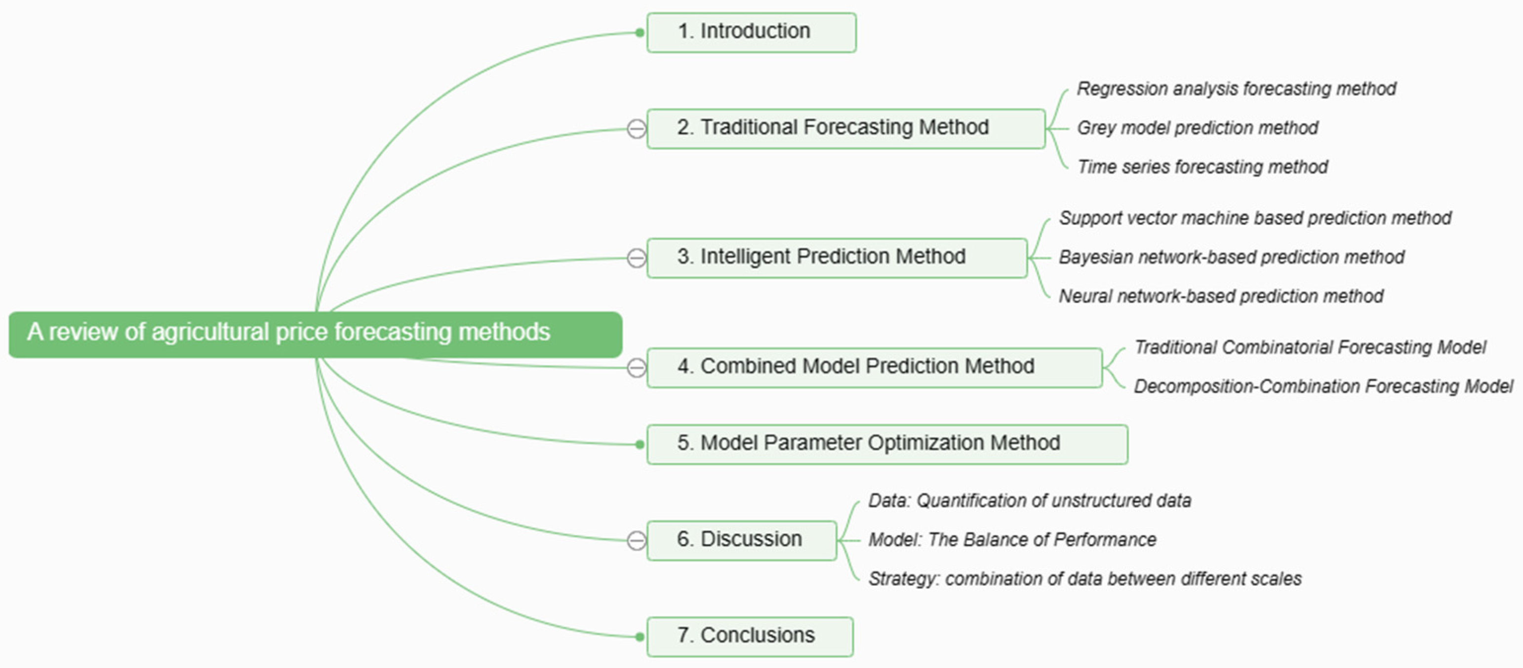
This paper describes the development of agricultural product price forecasting methods from single model to combination model, from traditional forecasting methods to intelligent forecasting methods. An introduction of the advantages and disadvantages of different methods with specific examples is presented and the future development trend of agricultural product price prediction methods is discussed. This paper analyzes and discusses the development status of agricultural price forecasting methods on the basis of reviewing the history of the development of this field. It summarizes the current problems and challenges faced by agricultural price forecasting methods, with a view to providing certain help and guidance for the development of the field of agricultural price forecasting. Figure 1 shows the structure of this paper.

2. Traditional Forecasting Method

2.1. Regression Analysis Forecasting Method

Regression analysis was founded by Galton, a famous British anthropologist and statistician, when he studied the paternal height relationship in the UK. In 1917, Moore [11] marked the shift from qualitative to quantitative methods for agricultural price forecasting by constructing a multiple linear regression model to forecast cotton production and prices. Regression analysis predicts prices by constructing a mathematical model between prices and influencing factors. The regression analysis method mainly includes linear regression model (LR), generalized linear regression model (GLR), nonlinear regression model (NLR), multiple adaptive regression splines (MARS), generalized additive model (GAM), etc. Limitations and Challenges: Regression models require a substantial amount of data to estimate model parameters accurately and reliably. They also assume that data are devoid of errors, outliers, and multicollinearity (high correlation among explanatory variables). If the data exhibit nonlinearity, seasonality, or cyclical patterns, or if there are structural changes or external shocks in the data-generating process, regression models might struggle to perform effectively. Regression models may also suffer from overfitting (fitting noise in the data rather than the signal) or underfitting (failure to capture the complexity of the data) issues, thereby impacting their predictive performance and generalization ability. Suitability: Regression models are suitable for short-term or medium-term forecasting problems where explanatory variables are known or can be reasonably estimated. They are also appropriate for problems where the response variable maintains a linear or simple nonlinear relationship with explanatory variables, and where the data pattern remains relatively stable and consistent over a period of time.

Ma et al. [12] established a VAR model to predict the short-term price of hogs based on the analysis of factors affecting hog prices. The results indicate that the VAR model performs well in predicting short-term prices of live pigs. But the prediction performance was poor when medium- and long-term forecasts were made for hog prices. Ge et al. [13] studied changes in corn prices and factors affecting them. They developed two types of models to forecast maize prices: A univariate nonlinear regression model using time as the independent variable and a multiple linear regression model incorporating production, consumption, import, and export volumes as independent variables. While the univariate nonlinear regression models provide reasonable corn price predictions, they lack a comprehensive examination of the intricate internal factors driving price changes. Consequently, the accuracy of these predictions is significantly compromised, rendering them suitable only for rough estimations. The foundational assumption of local pattern independence leads to some deviation when applying the regression analysis forecasting equation to medium- to long-term predictions. Furthermore, the complexity of factors influencing agricultural commodity prices poses challenges in encompassing all relevant variables during the modeling process. Nonetheless, the regression analysis method excels in revealing intrinsic patterns, relationships, and correlations among factors, contributing to its relatively high precision. Its straightforward comprehension and applicability in refining basic models make it a popular choice for short-term agricultural commodity price forecasting.

2.2. Gray Model Prediction Method

Gray model is a method for predicting systems containing uncertainties. This method is a semiparametric model that uses a small amount of data to construct differential equations describing trends in the data. The goal is to estimate the parameters of the equation using least squares and use it to predict future values of the variable. Some examples of gray models are GM (1, 1), GM (2, 1), and DGM (2, 1). Limitations and Challenges: Gray models require the data to have a degree of regularity and monotonicity, meaning that they steadily increase or decrease over time. They also assume that the data have an exponential law distribution, which means they grow or decay exponentially over time. Gray models may not work well if the data have irregular, non-monotonic, or non-exponential patterns, or if there are sudden changes or fluctuations in the data. Gray models may also suffer from low accuracy and poor adaptability, which affects their predictive performance and robustness. Applicability: Gray models are suitable for long-term forecasting problems where data are scarce or incomplete. They are also suitable for problems where variables have smooth and monotonic trends, and where data patterns are relatively simple and stable over time.

Luo Han Guo is a kind of fruit produced in Guangxi, China. Feng et al. [14] constructed a GM (1, 1) model to predict its price. It was found that the GM (1, 1) model could better portray its price change pattern due to its high in-sample simulation accuracy. It is concluded that the GM (1, 1) model has the advantages of requiring less data, high fitting and prediction accuracy, and easy programming implementation in the prediction problem for the price of Luo Han Guo, relative to the prediction models, such as regression models and time series models, and can provide a scientific reference for the prediction of the price of Luo Han Guo.

2.3. Time Series Forecasting Method

Time series analysis is a commonly used univariate forecasting method, which refers to a statistical method of modeling and analyzing agricultural commodity prices based on the regularity presented by the price itself over time, and extrapolating future data from existing data. The time series analysis method mainly includes autoregressive moving average (ARMA), autoregressive integrated moving average (ARIMA), seasonal autoregressive integrated moving average (SARIMA), autoregressive conditional heteroskedasticity (ARCH), generalized autoregressive conditional heteroskedasticity (GARCH), etc.

The advantage of time series analysis is that it is simple and straightforward. It relies entirely on historical data, and the time series methodology is a very flexible or short-term forecasting. The method performs well when the data show clear seasonal, trend, and cyclical patterns. Models and forecasts are created without the need to consider other influencing factors. Time series forecasting methods assume that the future pattern of change is the same as the historical pattern of change, but in practice, many times they are affected by external factors, leading to biased or failed forecasts. Climate change, policy implementation, and unforeseen events may lead to structural changes in the time series, making historical data not a good reflection of the future. The method requires complex steps, such as smoothness testing of the data, parameter estimation and model selection, which often require specialized knowledge and skills and can be subjective and uncertain. For example, an ARIMA model requires determining the values of p, d, and q. These values may affect model fitting effectiveness and forecasting accuracy. In addition, time series forecasting methods often suffer from error accumulation when performing multi-step forecasts, resulting in poor long-term forecasts. For example, if a moving average method is used to forecast data at several points in the future, data from earlier forecasts will need to be used as input, which will shift the error from earlier to later, making the forecasts increasingly inaccurate.

Table 1. Common time series analysis methods.

Model	Principle	Characteristic	Reference
AR (Autoregressive Model)	The AR model assumes that the current observations are a linear combination of past observations and uses historical observations to predict future values.	Capturing the dynamic properties and evolutionary trends of time series; handling time series data with long memory.	[15]
MA (Moving Average Model)	Reflects new observations by constantly updating the moving average. A weighted average of the mean, white noise errors, and their lagged values.	Capable of capturing the randomness and uncertainty of price fluctuations, especially when market supply and demand conditions are unstable.	-
ARIMA (Autoregressive Integrated Moving Average)	The basic principle of the ARIMA model is to use past data points, errors, and difference operations to predict future data points. The model minimizes the prediction error by adjusting the parameters of the autoregressive coefficients, moving average coefficients, and difference operations.	Ability to capture time series trending and seasonality. Essentially only captures linear relationships, not nonlinear relationships. It is required that the timing data are stable or are stable by differential differentiation.	[16]
ES (Exponential Smoothing)	It is based on the principle of using historical data to predict future trends by constantly adjusting the weights in order that the most recent data have a greater impact on the prediction results to reflect the trend and periodicity of the time series data.	It can reduce the noise and seasonality of the time series, thus improving prediction accuracy and stability. Predicting new trends and cycles requires constant updating of the model. The choice of smoothing constants is sensitive and less effective for time series with strong periodic fluctuations.	[17,18]

summarizes commonly used forecasting methods for time series analysis.

3. Intelligent Prediction Method

Traditional agricultural price forecasting methods, such as regression analysis, time series forecasting, and gray models, are usually applicable to the situation where the variables are independent, the data obey normal distribution, and there is a linear or simple nonlinear relationship. However, realistic agricultural price forecasting often fails to meet these conditions, and often presents complex problems, such as high dimensionality, small sample size, and nonlinearity.

Compared with econometric and mathematical-statistical methods, intelligent forecasting methods have fewer restrictions and assumptions in modeling and can effectively model nonlinear relationships in price series. Traditional machine learning methods, such as decision trees, support vector machines, and plain Bayes, have the advantages of simplicity, fast training and robustness, but they have limited ability to handle complex nonlinear relationships, require manual selection and extraction of features, and have insufficient generalization ability. Deep learning models, with their powerful expression and feature extraction capabilities, can extract effective feature information from the original sequence without relying on feature engineering and have better processing ability for nonlinear relationships in the sequence when supervision is effective, data quantity is sufficient, and data quality is high. However, the deep learning method has limitations, such as high data volume requirement, difficult parameter adjustment, easy overfitting, and poor interpretability. This module describes two traditional machine learning methods, support vector machines and plain Bayes, and the application of neural network methods in agricultural price prediction.

3.1. Support Vector Machine-Based Prediction Method

The support vector machine (SVM) is a machine learning approach rooted in statistical learning theory [19]. It hinges on VC dimensional theory, the principle of structural risk minimization [20,21], and represents the pioneering algorithm grounded in geometric distance [22]. Serving as a small-sample learning technique with a robust theoretical foundation, an SVM’s final decision function is influenced by only a handful of support vectors. Its computational complexity hinges on these vectors rather than the sample space’s dimensionality, sidestepping the so-called “dimensional disaster”. Wang et al. [23] harnessed SVM to predict the nonlinear facet of garlic prices, coupling it with ARIMA for linear price prediction, yielding accurate results. Nevertheless, SVM does have drawbacks, including diminished performance when data features (dimensions) surpass the sample size, sensitivity to parameters and kernel functions. Consequently, approaches like parameter optimization are frequently employed to enhance SVM prediction performance. Duan et al. [24] employed a genetic algorithm to identify optimal parameter combinations for a support vector regression model. With these optimized parameters, they constructed a support vector regression model for predicting fish prices, yielding precise outcomes with minor errors. SVR’s remarkable ability to manage high-dimensional, nonlinear, and small-sample data positions is a vital technique in agricultural price prediction.

3.2. Bayesian Network-Based Prediction Method

A Bayesian network is essentially a directed acyclic graph that uses probabilistic networks to make uncertainty inferences. The excellence of Bayesian networks in solving agricultural price forecasting as well as other agricultural problems stems mainly from the following key features: (1) Bayesian networks can handle incomplete datasets; (2) Bayesian networks allow one to understand the relationships between variables and quantify the strength of these relationships; (3) the ability to combine quantitative and qualitative data; (4) the ability to combine expert knowledge and data into Bayesian network; and (5) Bayesian methods can relatively easily avoid data overfitting during the learning process. Putri [25] used Bayesian network algorithms as a data mining classification method to predict pepper commodity prices in Bandung region based on weather information. One disadvantage of Bayesian networks is that they do not support ring networks [26], which would weaken the robust inference capability of the network, and this limitation is not friendly to static Bayesian networks. Dynamic Bayesian network (DBN) is a dynamic model amalgamating probability theory and influence diagram. It combines a time-varying hidden Markov model with a traditional static Bayesian network, capturing benefits from both while sidestepping their limitations through dynamic adaptability over time and the incorporation of new states [27]. Ma Zaixing [28] used the PC algorithm to learn from data, construct according to expert knowledge, and combine expert knowledge and PC algorithm to perform structural learning. After obtaining the initial structure, he adjusted the obtained initial structure to obtain the network structure of the model, and then used the EM algorithm to perform parameter learning. Moreover, he obtained a complete dynamic Bayesian network model for price prediction, and selected the best model based on the prediction results to predict the price and output of live pigs. The results show that the prediction effect is better than the control group’s ARIMA, SVM, and BP neural network models.

3.3. Neural Network-Based Prediction Method

Neural networks are commonly referred to as artificial neural networks (ANN). They constitute a complex nonlinear network system composed of numerous processing units interconnected in a manner resembling biological neurons. Neural networks exhibit robust nonlinear fitting capabilities, enabling them to map intricate nonlinear relationships. Furthermore, their learning rules are simple, making them easily implementable on computers. They possess strong robustness, memory, nonlinear mapping abilities, and powerful self-learning capabilities, showcasing unique advantages in addressing agricultural commodity price prediction challenges. In 1987, Lapedes and Farber [29] pioneered the application of neural networks to forecasting, marking the inception of neural network predictions. In 1993, Kohzadi et al. [30] were among the first to employ feed-forward neural networks for predicting US wheat and cattle prices. They compared the predictive results with those from ARIMA, concluding that neural networks exhibited superior turning point prediction capabilities and achieved more accurate price forecasting.

As big data and artificial intelligence technology advance, neural networks find increasingly wide application in the agricultural domain [31]. In the realm of price prediction, prevalent neural network models are as follows (Table 2, along with examples, summarizes the applications of neural networks in agricultural commodity price prediction):

• Backpropagation (BP) Networks [32,33,34]: BP networks are easy to implement and understand. However, it is easy to fall into local optimal solutions and the training speed is relatively slow.
• Radial Basis Function Neural Networks (RBFNN) [35,36]: A BP network is a global approximation of a nonlinear mapping, whereas an RBF network is a local approximation of a nonlinear mapping and is faster to train. RBF can handle complex nonlinear relationships and has good generalization ability. However, it is sensitive to the network structure and hyperparameters, and the training and tuning are relatively complicated. When the problem involves complex nonlinear relationships and there is enough training data, you can try to use RBF neural network.
• Long Short-Term Memory Networks (LSTM) [37,38]: LSTM neural network is a special kind of recurrent neural network that solves the problems of long-term dependency and gradient vanishing by introducing structures, such as forgetting gates, input gates, and output gates, to control the flow of information through the unit states. LSTM neural networks have the ability to memorize and capture long-term dependencies. Therefore, LSTM is a good choice when the prediction problem involves time series data, especially with long-term dependencies.
• Convolutional Neural Networks (CNN) [39]: CNN is a multi-layer feed-forward neural network that extracts local and global features from data through structures, such as convolutional, pooling, and fully connected layers to enable automatic feature learning and abstraction. In price prediction tasks, CNNs can learn and capture important features, such as time series, data trends, periodicity, etc., in the input data. Market prices are usually affected by a combination of several factors, and CNNs can better handle these complex nonlinear relationships.
• Chaos Neural Networks (CNN) [40,41]: Chaos neural network (CNN) is a kind of intelligent information processing system that combines chaos theory and neural network. Chaotic neural networks exploit the sensitivity and unpredictability of chaotic phenomena to enhance the learning and generalization capabilities of neural networks, thus improving the accuracy of prediction and modeling. By introducing methods, such as chaotic noise or logistic maps, chaotic neural networks are able to avoid neural networks from falling into local minima to a certain extent, thus speeding up the training process and increasing the convergence rate.
• Extreme Learning Machines (ELM) [42]: The extreme learning machine is a feed-forward neural network that was first proposed by Professor Huang Guangbin of Nanyang Technological University in Singapore in 2006. ELM has the advantages of fast training, high generalization ability, and simple implementation.
• Wavelet Neural Networks (WNN) [43,44]: Wavelet neural network (WNN) is a method based on wavelet transform and neural network. By decomposing the original data into wavelet coefficients at different scales, it is able to effectively extract a variety of features in the data, such as trend, cycle, seasonality, etc. WNN combines the powerful fitting ability of neural networks, which is capable of nonlinear mapping, thus achieving accurate prediction of future prices. However, high complexity and high data requirements are the unavoidable drawbacks of this method.

Table 2. Application examples of neural network-based price forecasting for agricultural products.

Reference	[32]	[35]	[38]	[39]	[41]	[42]	[44]
Models/Algorithms	BPNN	RBFNN	LSTM	CNN	Chaotic neural networks	ELM	WNN
Characteristic	Strong nonlinear mapping ability, high self-learning and self-adaptive ability, ability to apply learning outcomes to new knowledge, and certain fault tolerance. Research results show that the BP neural network model has the long-term prediction ability for the futures market.	It has better approximation ability, classification ability, and learning speed than BP neural network, simple structure, concise training, fast learning convergence speed, can approximate any nonlinear function, and overcome the local minimum problem. Research results show that the influencing factors of soybean price are different at different price levels, and the construction of this model is beneficial to the prediction of soybean price.	It effectively overcomes the problem of gradient vanishing caused by the increase in network layers in RNN. This model is especially suitable for tasks with very long time intervals and delays, and has excellent performance. Research results show that parameter tuning has a large impact on the prediction effect of LSTM network model, and the main parameters with large impact include iteration times, learning rate, window size, and network layers. Compared with ARIMA model, MLP model and SVR model, LSTM network model has higher accuracy in prediction results.	The effectiveness of CNN in feature extraction and autonomous learning of nonlinear patterns makes it perform well in image classification and audio recognition tasks. This study reviews the factors that affect crop yield and proposes a 3D CNN model to predict future crop prices. The model helps decision-makers to better predict crop price trends and formulate strategic plans, select trade partners, reduce costs, and solve food insecurity issues.	The output of the network not only depends on the current input, but also on the past output. After training, the network will have better adaptability to nonlinear data and is very suitable for predicting complex, non-stationary, and nonlinear time series. The designed potato price time series prediction model based on dynamic chaotic neural network has clear advantages over ARMA model in prediction accuracy and performance.	The algorithm can randomly generate the input weights and hidden layer thresholds required by the neural network without multiple adjustments. As long as the number of hidden layer nodes is reasonable, a unique optimal solution can be obtained. Its parameter setting process is simple, does not need to be adjusted repeatedly, the training speed is significantly improved, and the prediction results are more accurate. Compared with traditional neural network learning algorithms (such as BP algorithm), it overcomes the disadvantage of falling into local optimum. This study uses PCA-ELM model to predict grain prices and achieves good prediction results.	Wavelet neural network combines the advantages of neural network and wavelet function, using Morlet wavelet as the hidden layer basis function, which can extract local dynamic features, and can build a local approximation feed-forward neural network, reduce the interference between nodes, and improve the prediction accuracy. This study uses wavelet neural network to predict the prices of two kinds of Chinese medicinal materials, Radix Codonopsis and Angelica sinensis, and the results show that the prediction error is very small and the prediction accuracy is very high.
Agricultural Product	Egg	Soybeans	Soybeans	Five different Crops	Potato	Grain	Chinese herbal medicine
Observed Features	Soybean meal price, cull chicken price, corn price, egg seedling price, duck egg price	Domestic Soybean Production, Soybean Imports, Global Soybean Production, Domestic Soybean Demand, Consumer Price Index, Consumer Confidence Index, Money Supply, Imported Soybean Port Delivery Prices	Price time series	Environmental, economic, and commodity trading data	Price time series	Total grain production, per capita grain consumption, average grain production price index, per capita disposable income of urban residents, consumer price index, grain sown area	Planting area, yield, province’s disaster area, hype factor, and market demand
Evaluation Method	Mean Absolute Percentage Error	Mean Absolute Percentage Error, Relative error	Mean Absolute Error, Root Mean Square Error, Mean Absolute Percentage Error, R-Square	Mean Absolute Error, Root Mean Square Error, Mean Absolute Percentage Error	Mean Square Error	Mean Square Error	Relative error

Table 2. Application examples of neural network-based price forecasting for agricultural products.

Reference	[32]	[35]	[38]	[39]	[41]	[42]	[44]
Models/Algorithms	BPNN	RBFNN	LSTM	CNN	Chaotic neural networks	ELM	WNN
Characteristic	Strong nonlinear mapping ability, high self-learning and self-adaptive ability, ability to apply learning outcomes to new knowledge, and certain fault tolerance. Research results show that the BP neural network model has the long-term prediction ability for the futures market.	It has better approximation ability, classification ability, and learning speed than BP neural network, simple structure, concise training, fast learning convergence speed, can approximate any nonlinear function, and overcome the local minimum problem. Research results show that the influencing factors of soybean price are different at different price levels, and the construction of this model is beneficial to the prediction of soybean price.	It effectively overcomes the problem of gradient vanishing caused by the increase in network layers in RNN. This model is especially suitable for tasks with very long time intervals and delays, and has excellent performance. Research results show that parameter tuning has a large impact on the prediction effect of LSTM network model, and the main parameters with large impact include iteration times, learning rate, window size, and network layers. Compared with ARIMA model, MLP model and SVR model, LSTM network model has higher accuracy in prediction results.	The effectiveness of CNN in feature extraction and autonomous learning of nonlinear patterns makes it perform well in image classification and audio recognition tasks. This study reviews the factors that affect crop yield and proposes a 3D CNN model to predict future crop prices. The model helps decision-makers to better predict crop price trends and formulate strategic plans, select trade partners, reduce costs, and solve food insecurity issues.	The output of the network not only depends on the current input, but also on the past output. After training, the network will have better adaptability to nonlinear data and is very suitable for predicting complex, non-stationary, and nonlinear time series. The designed potato price time series prediction model based on dynamic chaotic neural network has clear advantages over ARMA model in prediction accuracy and performance.	The algorithm can randomly generate the input weights and hidden layer thresholds required by the neural network without multiple adjustments. As long as the number of hidden layer nodes is reasonable, a unique optimal solution can be obtained. Its parameter setting process is simple, does not need to be adjusted repeatedly, the training speed is significantly improved, and the prediction results are more accurate. Compared with traditional neural network learning algorithms (such as BP algorithm), it overcomes the disadvantage of falling into local optimum. This study uses PCA-ELM model to predict grain prices and achieves good prediction results.	Wavelet neural network combines the advantages of neural network and wavelet function, using Morlet wavelet as the hidden layer basis function, which can extract local dynamic features, and can build a local approximation feed-forward neural network, reduce the interference between nodes, and improve the prediction accuracy. This study uses wavelet neural network to predict the prices of two kinds of Chinese medicinal materials, Radix Codonopsis and Angelica sinensis, and the results show that the prediction error is very small and the prediction accuracy is very high.
Agricultural Product	Egg	Soybeans	Soybeans	Five different Crops	Potato	Grain	Chinese herbal medicine
Observed Features	Soybean meal price, cull chicken price, corn price, egg seedling price, duck egg price	Domestic Soybean Production, Soybean Imports, Global Soybean Production, Domestic Soybean Demand, Consumer Price Index, Consumer Confidence Index, Money Supply, Imported Soybean Port Delivery Prices	Price time series	Environmental, economic, and commodity trading data	Price time series	Total grain production, per capita grain consumption, average grain production price index, per capita disposable income of urban residents, consumer price index, grain sown area	Planting area, yield, province’s disaster area, hype factor, and market demand
Evaluation Method	Mean Absolute Percentage Error	Mean Absolute Percentage Error, Relative error	Mean Absolute Error, Root Mean Square Error, Mean Absolute Percentage Error, R-Square	Mean Absolute Error, Root Mean Square Error, Mean Absolute Percentage Error	Mean Square Error	Mean Square Error	Relative error

4. Combined Model Prediction Method

In practical forecasting applications, due to different modeling mechanisms and starting points, usually the same problem can have different forecasting methods. Different forecasting methods provide different useful information, have their own advantages and disadvantages, and they are not mutually exclusive, but interlinked and complementary to each other. A more scientific approach is to combine a number of different forecasting methods appropriately, thus forming the so-called combined forecasting method. Combination forecasting model is a combination of two or more models to forecast variables, which can make great use of sample data information, overcome the shortcomings such as single model is more influenced by random factors, and be more comprehensive and accurate, which will facilitate the synthesis of useful information provided by various methods as well as improve the accuracy of forecasting. Combinatorial forecasting is an important research branch in the field of forecasting, and since Bates and Granger [45] first proposed the theoretical system of combinatorial forecasting in 1969, the method has then received extensive attention from scholars at home and abroad. There are various ways to classify the combinatorial forecasting models. In order to clarify the combinatorial forecasting models in more detail, this study introduces them into two categories: “traditional combinatorial forecasting models” and “decomposition-combination”-based forecasting models.

Table 3. Examples of application of integration method.

Reference	[46]	[23]	[47]	[48]	[49]	[50]
Integration Method	Different weights are assigned according to the prediction error of a single model and then summed	Equal weighting method	Nonlinear combination of different prediction results by BP model	Equal weighting method	Equal weighting method	Equal weighting method
Application Examples	ARIMA forecasting model, GM (1,1) forecasting model, and combined forecasting model were used to forecast the wholesale market price of potatoes in 2020, and the results of ARIMA and GM were combined linearly to obtain the final forecast value	An ARIMA-SVM combined forecasting model is established to forecast garlic prices, and the prediction results of ARIMA and SVM are summed to obtain the final forecast value	A combined AttLSTM-ARIMA-BP forecasting model to forecast corn prices	The vegetable price data were decomposed into seasonal, trend, and residual components using the STL method. In this case, the derived variables of price are created in the residual component. Next, the input variables are learned through the attention layer and attention weights are assigned to all input variables. Input variables with attention weights assigned are learned through the LSTM model and vegetable prices for the next month are predicted	First, decompose the price series into nonlinear uptrend, seasonal trend, cyclic fluctuation trend, and random fluctuation trend using wavelet analysis, then predict the nonlinear uptrend using support vector machine, predict the seasonal trend, cyclic fluctuation trend and arbitrary fluctuation trend using ARIMA, and finally sum up the predicted values to get the predicted value	First, the empirical modal decomposition (EMD) method is used to decompose and integrate the monthly pork market prices into three modules: High-frequency part, low-frequency part, and residual term to solve the volatile and non-stationary problem. On the basis of this method, support vector machine (SVM) is applied to forecast each of the three integrated modules to solve the nonlinear problem. Finally, the prediction results of the three integrated modules are integrated again to reconstruct the pork market price prediction value
Agricultural Product	Potato	Garlic	Corn	Vegetable	Chinese cabbage	Pork
Observed Features	Price time series	Price time series	Food prices in different geographical areas	Vegetable prices, weather information for major production areas, and vegetable import and export data	Price time series	Price time series
Evaluation method	The study used evaluation methods, such as absolute error and absolute percentage error, to evaluate the model performance. The conclusion is that the established combination model has better prediction effect, and its prediction accuracy and stability are better than the two single models.	The study used RMSE to evaluate the model performance. The results of the study showed that the accuracy of the hybrid ARIMA-SVM model for garlic price prediction is better than the single ARIMA and SVM models and can be used as an effective method for predicting short-term prices of garlic.	The study evaluates the performance of the model using MAPE, RMSE, and MAE. The results of the study show that the model is not only suitable for price forecasting during periods of stable data changes, but also gives accurate forecasts when the price changes are large.	The study evaluated the model using RMSE and MAPE. The results of the study show that the LSTM model incorporating the STL method (STL-LSTM) improves the prediction accuracy by 12% compared to the LSTM model without the STL method and resolves the prediction lag caused by high seasonality.	The study evaluates the model using MAPE and RMSE. The results of the study show that the combined model adequately analyzes the various trends in the price series and its forecasting performance is better than the single ARIMA and SVM model.	The study evaluated the model using RMSE, MAPE, and directional symmetry methods. The results show that the combined model EMD-SVM fully considers the characteristics of randomness, periodicity, and trend of monthly pork market price, explains the inner meaning of price fluctuation, and not only shows high prediction accuracy, but also can better grasp the direction of the pork price trend, which can provide new ideas and methods for the price prediction of pork market.

summarizes several examples of combination models.

4.1. Traditional Combinatorial Forecasting Model

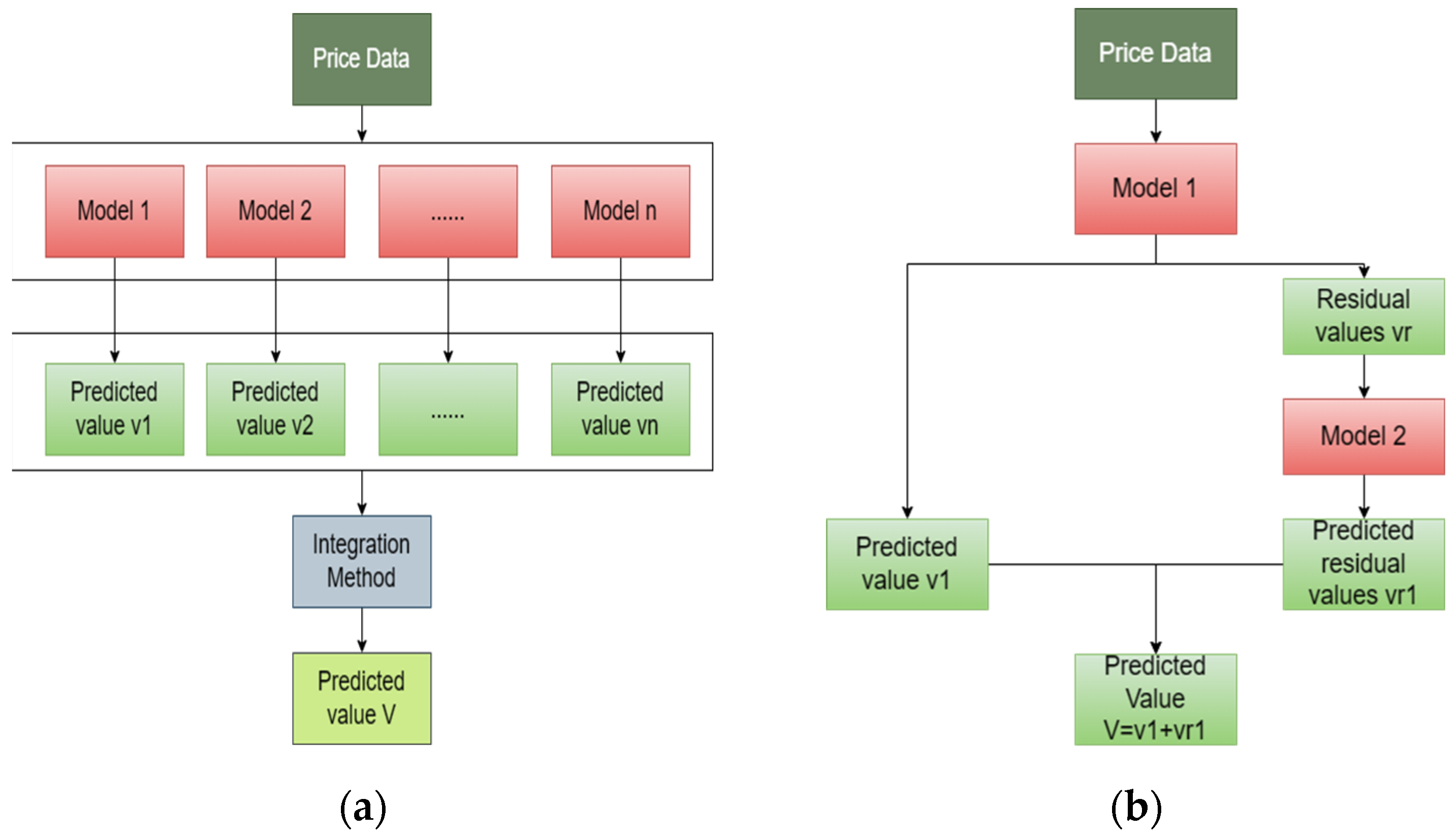
The principle of traditional ensemble models involves utilizing different forecasting models to predict agricultural commodity prices separately. Eventually, these individual predictions are combined using specific integration methods to yield the overall forecasted outcome (Figure 2a). Figure 2b provides an example of a traditional ensemble forecasting model. In this instance, two distinct models are employed to predict price data and residuals separately. Subsequently, their predictions are added together to produce the final forecasted outcome [23].

4.2. Decomposition-Combination Forecasting Model

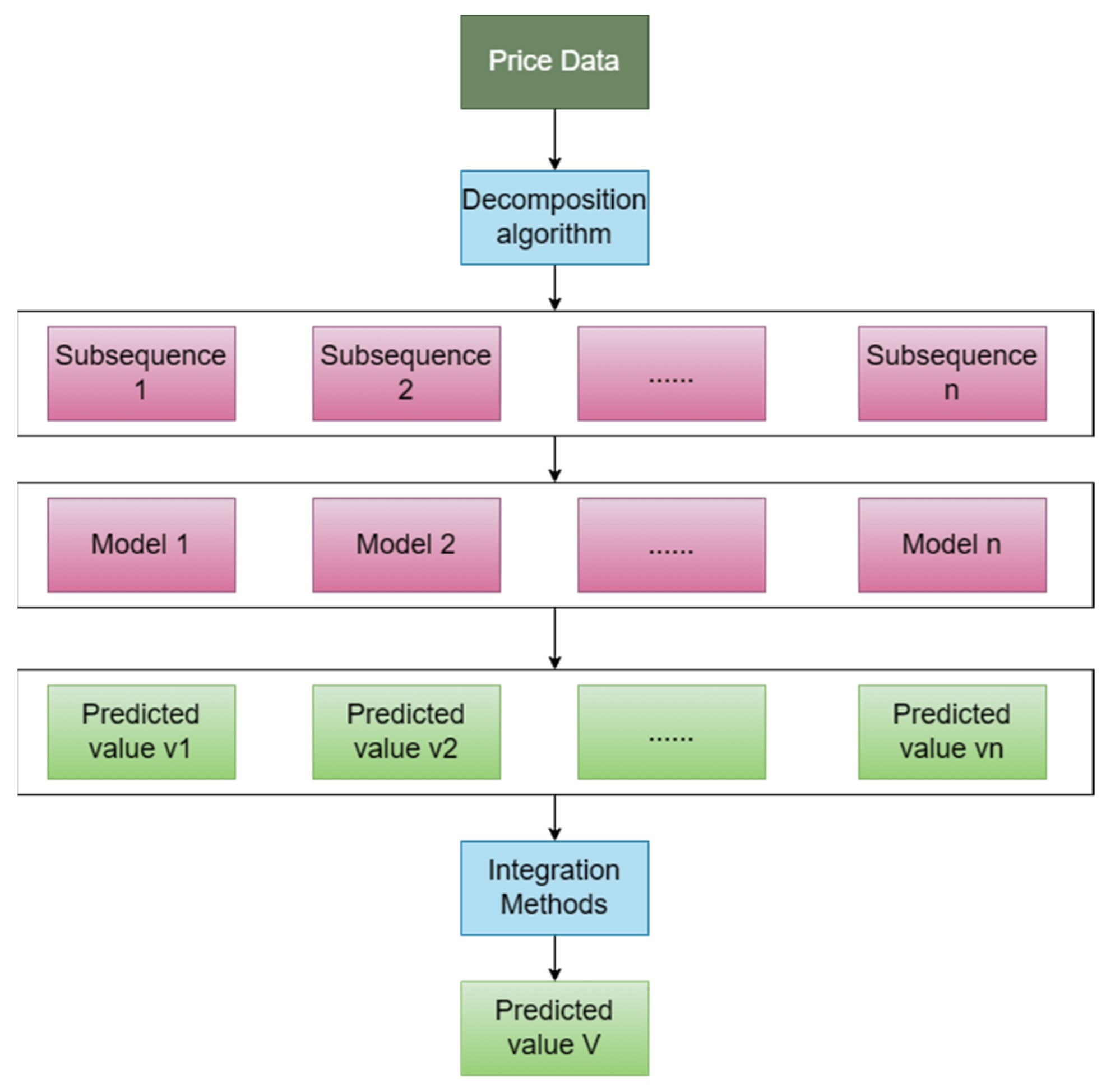
The “decomposition-ensemble” forecasting method is based on the multi-scale decomposition of original complex time series data. It dissects the fluctuation patterns and trend regularities of intricate systems at various scales. By understanding the inherent operational patterns of the system, predictive research is conducted, leading to a significant enhancement in forecasting performance. The decomposed ensemble combination model refers to splitting the intricate price sequence into several simpler sub-sequences. Each sub-sequence is individually forecasted using models, and the predictions of these sub-sequences are then integrated to obtain the forecasted values of the original sequence (Figure 3). The core of this methodology lies in selecting effective data decomposition tools. Common decomposition methods include seasonal decomposition [48], wavelet decomposition [49], empirical mode decomposition [50], and variational mode decomposition [51]. The advantages of the “decomposition-ensemble” combination forecasting model lie in its ability to leverage information across different scales. It mitigates the impact of features like noise, trends, and cycles inherent in complex data, thus enhancing prediction accuracy and robustness. However, a drawback of the “decomposition-ensemble” combination forecasting model is the need to determine suitable data decomposition tools and integration methods; otherwise, it could affect the extraction and reconstruction of data features.

Table 4. Common decomposition methods.

Decomposition Method	STL Seasonal Decomposition	Wavelet Decomposition	Empirical Modal Decomposition	Variational Modal Decomposition
Characteristics	It decomposes the price series into trend, seasonal, and residual components, which can handle non-stationary time series and is suitable for forecasting agricultural prices with significant seasonality.	The multi-scale decomposition of price series using wavelet function can extract features with different frequencies, which is suitable for price prediction of agricultural products with multiple periodicity and abrupt change points.	It decomposes the price series into several eigenmodular functions (IMFs) and residual terms, which can handle nonlinear and non-stationary time series adaptively and is suitable for forecasting agricultural prices with complex volatility characteristics.	It decomposes the price series into several eigenmodal functions (IMFs), which can effectively avoid the pattern mixing phenomenon in the EMD decomposition method and improve the decomposition effect, and is suitable for price prediction of agricultural products with high-frequency and low-frequency components.

summarizes the commonly used decomposition methods.

Whether it is a traditional ensemble forecasting model or a “decomposition-ensemble”-based combination forecasting model, the effectiveness of combination forecasting relies to a certain extent on the chosen integration method, namely, different weight design schemes. Utilizing effective integration methods may even lead to superior combination forecasting results compared to the best individual forecasts.

Table 5. Common integration methods.

Integration Method	Equal Weighting Method	Minimum Variance Method	Dominance Matrix Method	Least Squares Estimation Method
Principle	The equal weight method refers to assigning the same weights to the prediction results of all models and then averaging them to obtain the final prediction results.	The minimum variance method refers to giving a larger weight to the model with small variance based on the variance of the historical prediction errors of each model, and then finding the weighted average to obtain the final prediction results.	The dominance matrix method refers to constructing a dominance matrix based on the degree of prediction dominance of each model in different time periods, and then giving corresponding weights to each element of the matrix according to its size, and then finding the weighted average to get the final prediction results.	The least squares estimation method refers to estimating the optimal weight coefficients based on the least squares relationship between the historical prediction results and the true values of each model, and then finding the weighted average to obtain the final prediction results.
Characteristics	The advantage of this approach is that it is simple and easy to implement. The disadvantage is that it does not reflect the predictive power and accuracy of different models and may lead to inefficient combinations.	The advantage of this approach is that it can reduce the variance of the combined predictions and improve stability. The disadvantage is that it cannot take into account the correlation between models and may lead to over reliance on certain models.	The advantage of this approach is that it can synthesize the performance of different models over different time periods, and the disadvantage is that constructing the dominance matrix requires a certain amount of subjective judgment and experience.	The advantage of this method is that the optimal solution can be obtained using statistical methods, and the disadvantage is that certain assumptions, such as linear relationship and normal distribution, need to be satisfied.
Reference	[53]	[54]	[55]	[56]

summarizes several commonly used integration methods. These methods all fall under linear integration approaches, as they involve multiplying the prediction results of different models by weight coefficients and then summing them to obtain the final forecast result. Linear combination methods are common integration techniques, but they are not the sole ones. There are also nonlinear combination methods, such as neural networks, support vector machines, and fuzzy logic. These methods employ more complex functions to combine predictions from different models. Han et al. [52] found that nonlinear combination forecasting methods generally outperform linear combination methods. Among them, neural network-based nonlinear combination forecasting methods exhibit higher predictive accuracy than other optimal combination methods. Guo [47] constructed an AttLSTM-ARIMA-BP combination model for predicting corn prices. This model utilizes a BP model to train LSTM and ARIMA prediction results to generate the final forecast value, and the results demonstrate favorable predictive performance.

5. Model Parameter Optimization Method

When establishing agricultural commodity price forecasting models, the initially set or obtained parameters are likely not optimal or near optimal. In these cases, parameter optimization is necessary to attain an improved predictive model. Common methods for parameter optimization include cross validation, grid search, genetic algorithms, particle swarm optimization, and simulated annealing. Additionally, algorithms inspired by collective behaviors of social insects or group animals, such as bee colony algorithms, ant colony algorithms, and fish swarm algorithms, are frequently employed to optimize model parameters based on biological collective behavior patterns. Lu [57] employed the particle swarm optimization (PSO) algorithm to develop a PSO-BP forecasting model for vegetable retail prices. Zhang [35] proposed a hybrid algorithm called GDGA, which combines the best features of global and local search methods. Results indicate that the proposed hybrid GDGA algorithm outperforms multivariate linear regression and pure GA methods in terms of predictive performance and converges faster than pure genetic algorithms (GA). Experimental findings demonstrate that compared to traditional BP methods, the PSO-BP approach can overcome overfitting and local minimum issues, effectively reducing training errors and enhancing predictive accuracy.

With increasing research, investigators have gradually found that predictive models utilizing combination optimization algorithms tend to exhibit superior forecasting performance compared to single optimization algorithms. Combination parameter optimization algorithms offer several advantages: they handle complex optimization problems involving discrete, nonlinear, and multi-modal functions better than single parameter optimization algorithms, which often require certain conditions or assumptions like differentiability and convexity. Combination parameter optimization algorithms are more effective at avoiding local optima, as single parameter optimization algorithms are often susceptible to initial value influence, leading to slow convergence or getting stuck in suboptimal solutions. Moreover, combination parameter optimization algorithms can flexibly adapt to diverse problem characteristics and requirements. For instance, they can employ various fitness functions, crossover-mutation strategies, and neighborhood structures. In contrast, single parameter optimization algorithms are usually more rigid and uniform, making adjustment and improvement challenging. Of course, combination parameter optimization algorithms also have drawbacks, such as higher computational complexity, challenging theoretical analysis, and sensitivity to parameter choices. Therefore, in practical applications, appropriate optimization algorithms should be selected based on specific problem features and objectives, and adjustments and improvements should be made accordingly.

Table 6. Common optimization methods and examples.

Optimization Methods	Cross Validation	Grid Search	Genetic Algorithm	Particle Swarm Optimization	Simulated Annealing
Principle	Cross validation is a method to evaluate the performance of a model by dividing the dataset into several subsets, using one subset at a time as the test set and the other subsets as the training set, repeating several times, and then calculating the average performance metrics of the model on the different test sets.	Grid search is a method to find the optimal model parameters by traversing a given range and combination of parameters, cross validating each combination of parameters, and then selecting the combination of parameters with the best cross validation performance as the optimal parameters, the marker values, and their corresponding optimal parameter values.	A genetic algorithm is a heuristic optimization algorithm that simulates the process of biological evolution in nature by continuously updating a set of candidate solutions (called populations) through operations, such as selection, crossover, and mutation, until termination conditions are met.	Particle swarm optimization is a population intelligence-based optimization algorithm that simulates the foraging behavior of a flock of birds by adjusting the speed and position of each candidate solution (called particles) to move closer to the individual optimal solution and the global optimal solution.	Simulated annealing is a probability-based optimization algorithm that simulates the process of a solid substance reaching an energy minimum state during heating and cooling by randomly perturbing the current solution (called the state) and accepting or rejecting the new solution based on a probability (called the Boltzmann function) that decreases with temperature.
Characteristics	Cross validation can make effective use of limited data to avoid over- or under-fitting problems and can also be used to select optimal model parameters or features.	Grid search can systematically explore the parameter space and find the global optimal solution, but it is computationally expensive and cannot handle continuous parameters.	Genetic algorithms can handle nonlinear, multi-peaked, discrete or continuous optimization problems with strong global search capability and robustness, but convergence is slow and prone to fall into early convergence.	Particle swarm optimization has the advantages of fast convergence, few parameters, and simple and easy implementation of the algorithm, but it also has the problem of falling into local optimal solutions.	Simulated annealing can jump out of the local optimal solution and find the global optimal solution, which is suitable for combinatorial optimization problems, but it takes a longer time to adjust the parameters and cooling progress.
Application	For selecting the optimal model parameters or features, such as regularization coefficients, kernel functions, feature subsets, etc.	It is mainly used to find the optimal model parameters, such as penalty parameters and kernel function parameters of support vector machines, learning rate, and number of hidden layer nodes of neural networks.	Genetic algorithms have been widely used in the fields of combinatorial optimization, machine learning, signal processing, adaptive control, and artificial life.	It is mainly used for optimization of continuous problems, such as function optimization problems, neural network training problems, engineering design problems, etc.	The simulated annealing algorithm is a general-purpose optimization algorithm with theoretically probabilistic global optimization performance, which has been widely used in engineering, such as VLSI, production scheduling, control engineering, machine learning, neural networks, signal processing, and other fields.
Reference	[58]	[59]	[60]	[61]	[62]

summarizes several classic parameter optimization methods using examples to provide a comprehensive overview.

6. Discussion

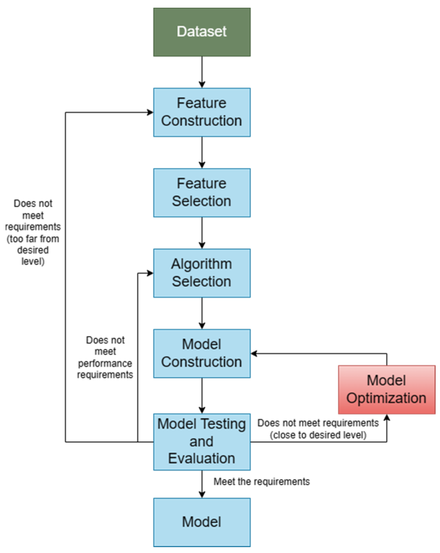
In the process of building agricultural price forecasting models (Figure 4), in addition to the key step of algorithm selection, processes such as feature selection, model construction, and model optimization are also crucial. In this paper, we explore possible research directions or methods to improve the performance of agricultural price forecasting from the perspectives of data, models, and strategies.

6.1. Data: Quantification of Unstructured Data

Unstructured data are data that have no fixed format or structure, such as text, images, audio, video, etc. The quantification of unstructured data can help extract useful information from it, discover hidden patterns, and support decision making and innovation. With the development of Internet technology, the amount of unstructured data is increasing day by day. The extraction and quantification of unstructured data information is especially important to improve the prediction accuracy of agricultural prices.

With the development and application of social media, farmers and consumers are increasingly influenced by online public opinion, leading to unreasonable planting or purchasing behavior, which has a complex impact on the price of agricultural products. The use of “text mining” technology to extract information from unstructured data not only enriches the feature information of agricultural price prediction models, but also improves the accuracy of prediction and compensates the shortcomings of neural network models that are difficult to interpret the output results. Moreover, adding sentiment scores to agricultural price prediction can effectively improve the prediction performance. Ye [63] used discussions in online professional communities to construct heterogeneous graphs, and finally, constructed HGLSTM for prediction. The experimental results showed that the prediction of hog prices using forum discussion data was effective. Drury [64] studied the application of text mining in agriculture and found that there are a large number of agricultural texts in agricultural research, such as scientific papers and news reports, which can be analyzed by text mining techniques to solve agricultural problems including agricultural price prediction. Drury concluded that although text mining techniques are relatively mature, text mining has not been fully utilized in the field of agricultural price prediction. In recent years, research on text mining techniques in the field of price forecasting, including agricultural price forecasting, has gradually increased.

Table 7. Text Mining Based Price Prediction for Agricultural Products.

Reference	[65]	[66]	[67]
Application Examples	A text-based prediction framework is proposed that can effectively identify and quantify factors affecting agricultural futures based on a large number of online news headlines.	Proposing an effective prediction model using text data on social media—two-stage hybrid long- and short-term memory (TSH-LSTM).	Sentiment analysis was used to extract key information from web text from four perspectives: Compound sentiment, negative sentiment, neutral sentiment, and positive sentiment. These were constructed as features and fed into the oil price prediction model along with the oil price itself. Finally, we analyzed the impact from different perspectives and came up with some interesting findings.
Agricultural Product	Soybean	Soybean	Oil
Observed Features	Traditional variables, such as exports, imports, production, inventories, etc.; text-based variables, such as weather and policy factors.	Traditional variables as well as social media based text data.	Web-based Sentiment Analysis, oil price.
Conclusion	The results show that the identified influential factors and sentiment-based variables are effective, and the proposed framework performs significantly better in medium- and long-term forecasting than the benchmark model.	The empirical results indicate that the incorporation of the social media text feature helps improve forecasting performances. Specifically, the proposed TSH-LSTM is more accurate than univariate LSTM, multivariate LSTM, and eXtreme Gradient Boosting.	Using network information for oil price forecasting improves the accuracy and stability of forecasts.

summarizes several examples of price prediction based on text mining.

6.2. Model: The Balance of Performance

When evaluating the performance of agricultural price forecasting models, we need to consider several aspects, such as between the accuracy of forecast values and forecast trends, between model complexity and interpretability, and the combination of data between different scales. Balancing these factors is an important goal for the future development of agricultural price forecasting methods.

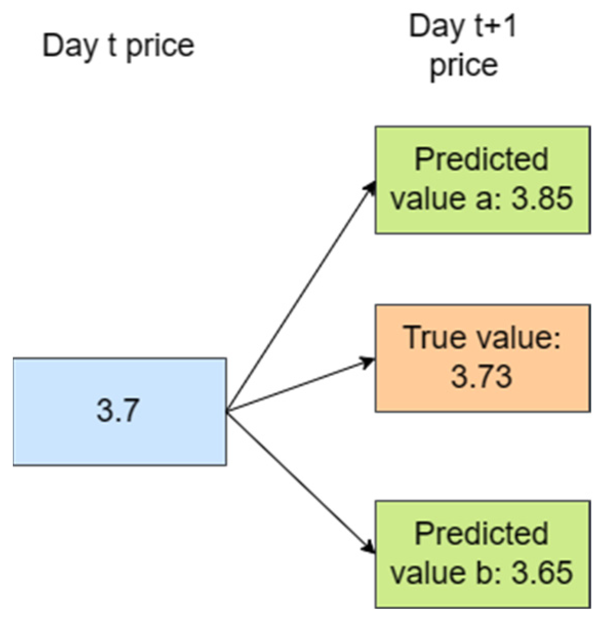
• Balancing Accuracy of Predicted Values and Predicted Trends. When evaluating the quality of forecast results, it is often assessed from two perspectives: predicted values and the forecasted trend (or rise and fall). For instance, for a certain agricultural commodity, the price on day t is 3.7, and the actual price on day t + 1 is 3.73. Predicted value a is 3.85, while predicted value b is 3.65. From an error perspective, predicted value b is closer to the true value than predicted value a. However, considering the forecasted trend, predicted value a is accurate, while predicted value b is opposite (Figure 5). Achieving precise predicted values and accurate forecasted trends does not necessarily conflict, but simultaneously achieving both can be challenging. In future research, ensuring the accuracy of both predicted values and forecast directions is a key issue to address. Moreover, the accuracy of the forecasted trend direction should be considered as a performance metric for future forecasting models, and methods like directional symmetry can be employed to measure the accuracy of the model’s forecast direction.
• Balancing Model Complexity and Interpretability. The effectiveness of agricultural commodity price forecasting also relies on striking a balance between model complexity and interpretability. Currently, certain machine learning and deep learning methods can handle nonlinear and intricate data relationships well, enhancing prediction accuracy. However, these methods also elevate model complexity and demand computational resources, diminishing model interpretability. In order to improve the explanatory performance of the model, some of the following methods can be used: using explainable machine learning algorithms, such as decision trees, linear regression, logistic regression, etc., which can visually demonstrate the relationship between features and target variables, as well as the importance and weight of the features; using feature engineering and feature selection techniques, pre-processing and downscaling of the raw data, extracting the most meaningful and influential features, and removing redundant and irrelevant features to make the model more concise and easy to understand; using model interpretation tools, such as LIME, SHAP, ELI5, etc., to interpret the prediction results of the model locally or globally, and to analyze the contribution and degree of influence of each feature on the prediction results, as well as the interaction effects between different features. Although the above methods can improve the interpretability of the model to some extent. However, for the time being, complexity and interpretability seem to be mutually exclusive, with more complex models also implying less interpretability. Therefore, how to maximize the interpretability of the model while ensuring its accuracy is a major challenge for future research in this area. This includes, among other things, research on model complexity, methods for establishing interpretability metrics, or the development of standards.

6.3. Strategy: Combination of Data between Different Scales

In general, people often use data with the same time scale for price forecasting, such as modeling daily data to obtain forecasts at a daily frequency. Some researchers have found that time series data of different time scales contain different amounts of information, and combining data from different time scales can enhance prediction performance. Ling et al. [68] were the first to attempt the combination of forecasts from multiple time scales, proposing a novel multi-time scale combination strategy for forecasting Chinese livestock product prices. The research results indicate that adopting this new combination approach can significantly improve prediction performance. Liwen et al. [69] proposed a multi-time scale combination strategy for predicting pork prices. Using daily prices as a base, weekly and monthly forecasts are transformed into daily frequency data, forming multi-time scale forecast results that reflect the multidimensional data generation process of price time series. Various multi-scale combination strategies were constructed to address short-, medium-, and long-term forecasting needs, investigating the matching relationship between forecast horizon and time scale. The research findings suggest that while multi-time scale combination strategies may not enhance short-term prediction performance, they can effectively improve accuracy in medium- and long-term forecasts.

But the strategy also has certain challenges. First, the time scale matching problem. How to choose a combination of different time scales and how to match the forecast step and time scale may be a challenge. Different time scales may have different trends and periodicities, and how to reasonably match these characteristics may require some empirical or methodological support. Second, considering multiple time scales may require the use of more sophisticated models to capture trends and relationships at different scales. This may lead to increased model complexity, requiring more parameter tuning and computational resources, as well as increased risk of overfitting. Finally, interpretive issues. Interpreting the predictions of a model can become more complex when models with multiple time scales are used. Understanding how different time scales interact with each other and how they collectively contribute to the predictions may become more difficult. In future research, there should be a stronger focus on exploring multi-time scale combination strategies and their application in multi-step forecasting of agricultural product prices.

7. Conclusions

Agricultural product price forecasting is a comprehensive, cross cutting, and dynamic research field. With the continuous development and changes in data sources, data types, data quality, data processing techniques, model construction techniques, and model evaluation techniques, agricultural product price forecasting methods will also be updated and improved. This paper systematically summarizes the development of agricultural price forecasting methods from traditional methods to intelligent methods, from single models to combined models. The possible future development trends are also discussed. Future research can explore the following aspects:

(1)

developing more effective unstructured data information extraction and quantification techniques, and using more data sources and data types to enrich the feature information of agricultural price prediction models;

(2)

finding more suitable combined model integration methods, such as using neural networks, to improve the effectiveness and efficiency of combined model prediction methods;

(3)

balancing model complexity and interpretability to improve model performance and practicality;

(4)

exploring the combination strategy of multiple time scales and its effectiveness and advantages in the application of multi-step forecasting of agricultural prices;

(5)

considering the accuracy of the trend direction of forecasting results as an indicator to evaluate the performance of forecasting models, while ensuring the accuracy of forecasting values and forecasting directions.

(6)

Mechanisms and methods for the construction of combined models for agricultural price forecasting need to be studied in depth, and the comparison and integration between different methods need to be strengthened to improve the accuracy and practicality of forecasting.

References

- Zheng, L. Model Construction and Empirical Study on Production and Consumption Forecasting of Major Agricultural Products in China. Master’s Thesis, University of Chinese Academy of Sciences, Beijing, China, 2013. [Google Scholar]
- Cao, Y.L.; Mohiuddin, M. Sustainable Emerging Country Agro-Food Supply Chains: Fresh Vegetable Price Formation Mechanisms in Rural China. Sustainability 2019, 11, 2814. [Google Scholar] [CrossRef]
- Zhang, D.; Liu, H.; Zhang, Y. Forecasting Chinese domestic soybean price based on Q-RBF neural network model. Soybean Sci. 2017, 36, 143–149. [Google Scholar] [CrossRef]
- Tothova, M. Main Challenges of Price Volatility in Agricultural Commodity Markets. In Methods to Analyse Agricultural Commodity Price Volatility; Springer: New York, NY, USA, 2011; pp. 13–29. [Google Scholar] [CrossRef]
- Xiao, X.Y.; Li, C.G. The price characteristics, problems and solutions of vegetables in China. Res. Agric. Mod. 2016, 37, 948–955. [Google Scholar] [CrossRef]
- Xu, L.; Zhang, Q.; Xu, S.W. Analysis of vegetable price increases in China since 2009. Food Nutr. China 2012, 18, 39–44. [Google Scholar] [CrossRef]
- Beckert, J. Where do prices come from? Sociological approaches to price formation. Socio-Econ. Rev. 2011, 9, 757–786. [Google Scholar] [CrossRef]
- Aguiar, D.R.; Santana, J.A. Asymmetry in farm to retail price transmission: Evidence from Brazil. Agribus. Int. J. 2002, 18, 37–48. [Google Scholar] [CrossRef]
- Ward, R.W. Asymmetry in retail, wholesale, and shipping point pricing for fresh vegetables. Am. J. Agric. Econ. 1982, 64, 205–212. [Google Scholar] [CrossRef]
- Gu, Z.; Zhang, Y. A study on the Influence Factors of Agricultural Prices based on Machine Learning—Taking oilseeds as an example. Price Theory Pract. 2023, 4, 122–126. [Google Scholar] [CrossRef]
- Moore, H.L. Forecasting the Yield and the Price of Cotton; Macmillan: New York, NY, USA, 1917. [Google Scholar]
- Ma, C.; Tao, J.P.; Liu, W. Pig Epidemic Network Concerns and Pork Price Volatility: Exacerbating or Curbing? J. Huazhong Agric. Univ. (Soc. Sci. Ed.) 2022, 6, 22–34. [Google Scholar] [CrossRef]
- Ge, Y.; Wu, H. Prediction of corn price fluctuation based on multiple linear regression analysis model under big data. Neural Comput. Appl. 2020, 32, 16843–16855. [Google Scholar] [CrossRef]
- Feng, F.; Wei, F.; Miu, J.H. Price Prediction of Traditional Chinese Medicine Siraitia grosvenorii Based on Grey System GM(1,1)Model. Guangxi Sci. 2012, 19, 15–20. [Google Scholar] [CrossRef]
- Cuaresma, J.C.; Hlouskova, J.; Kossmeier, S.; Obersteiner, M. Forecasting electricity spot-prices using linear univariate time-series models. Appl. Energy 2004, 77, 87–106. [Google Scholar] [CrossRef]
- Jadhav, V.; Chinnappa, R.B.; Gaddi, G. Application of ARIMA model for forecasting agricultural prices. J. Agric. Sci. Technol. 2017, 9, 981–992. [Google Scholar]
- Brown, R.G.; Meyer, R.F. The fundamental theorem of exponential smoothing. Oper. Res. 1961, 9, 673–685. [Google Scholar] [CrossRef]
- Wu, L.; Liu, S.; Yang, Y. Grey double exponential smoothing model and its application on pig price forecasting in China. Appl. Soft Comput. 2016, 39, 117–123. [Google Scholar] [CrossRef]
- Zhang, X.G. Introduction to Statistical Learning Theory and Support Vector Machines. Acta Autom. Sin. 2000, 26, 32–42. [Google Scholar]
- Sain, S.R. The Nature of Statistical Learning Theory; Taylor & Francis: Abingdon, UK, 1996; Volume 38, p. 409. [Google Scholar] [CrossRef]
- de Mello, R.F.; Ponti, M.A. Statistical learning theory. Mach. Learn. 2018, 75–128. [Google Scholar]
- Andrew, A.M. An Introduction to Support Vector Machines and Other Kernel-Based Learning Methods by Nello Christianini and John Shawe-Taylor, Cambridge University Press, Cambridge. Robotica 2000, 18, 687–689. [Google Scholar] [CrossRef]
- Wang, B.; Liu, P.; Chao, Z.; Junmei, W.; Chen, W.; Cao, N.; O’Hare, G.M.; Wen, F. Research on Hybrid Model of Garlic Short-term Price Forecasting based on Big Data. Comput. Mater. Contin. 2018, 57, 283–296. [Google Scholar] [CrossRef]
- Duan, Q.; Zhang, L.; Wei, F.; Xiao, X.; Wang, L. Time Series GA-SVR based Fish Price Prediction Model and Validation. Trans. Chin. Soc. Agric. Eng. 2017, 33, 308–314. [Google Scholar] [CrossRef]
- Nuvaisiyah, P.; Nhita, F.; Saepudin, D. Price prediction of chili commodities in Bandung regency using Bayesian Network. IJoICT 2018, 4, 19–32. [Google Scholar] [CrossRef]
- Ticehurst, J.L.; Letcher, R.A.; Rissik, D. Integration modelling and decision support: A case study of the Coastal Lake Assessment and Management (CLAM) Tool. Math. Comput. Simul. 2008, 78, 435–449. [Google Scholar] [CrossRef]
- Pearl, J. Graphical models for probabilistic and causal reasoning. Quantified Represent. Uncertain. Imprecision 1998, 1, 367–389. [Google Scholar] [CrossRef]
- Ma, Z. Prediction of Hog Price and Produce Based on Dynamic Bayesian Network. Master’s Thesis, Huazhong Agricultural University, Wuhan, China, 2019. [Google Scholar] [CrossRef]
- Lapedes, A.; Farber, R. Nonlinear Signal Processing Using Neural Networks: Prediction and System Modelling. 1987. Available online: https://www.osti.gov/servlets/purl/5470451 (accessed on 11 November 2022).
- Kohzadi, N.; Boyd, M.S.; Kermanshahi, B.; Kaastra, I. A comparison of artificial neural network and time series models for forecasting commodity prices. Neurocomputing 1996, 10, 169–181. [Google Scholar] [CrossRef]
- Liakos, K.G.; Busato, P.; Moshou, D.; Pearson, S.; Bochtis, D. Machine learning in agriculture: A review. Sensors 2018, 18, 2674. [Google Scholar] [CrossRef]
- Gao, Y.; An, S. Comparative Study on the Predictive Effect of the Price of Eggs in China—Comparative analysis based on BP neural network model and egg futures predictive model. Price Theory Pract. 2021, 4, 441. [Google Scholar] [CrossRef]
- Yu, Y.; Zhou, H.; Fu, J. Research on agricultural product price forecasting model based on improved BP neural network. J. Ambient Intell. Humaniz. Comput. 2018, 1–6. [Google Scholar] [CrossRef]
- Nasira, G.; Hemageetha, N. Vegetable price prediction using data mining classification technique. In Proceedings of the International Conference on Pattern Recognition, Informatics and Medical Engineering (PRIME-2012), Salem, India, 21–23 March 2012; pp. 99–102. [Google Scholar] [CrossRef]
- Zhang, D.; Zang, G.; Li, J.; Ma, K.; Liu, H. Prediction of soybean price in China using QR-RBF neural network model. Comput. Electron. Agric. 2018, 154, 10–17. [Google Scholar] [CrossRef]
- dos Santos Coelho, L.; Santos, A.A. A RBF neural network model with GARCH errors: Application to electricity price forecasting. Electr. Power Syst. Res. 2011, 81, 74–83. [Google Scholar] [CrossRef]
- Fang, X.; Wu, C.; Yu, S.; Zhang, D.; Ouyang, Q. Research on Short-Term Forecast Model of Agricultural Product Price Based on EEMD-LSTM. Chin. J. Manag. Sci. 2021, 29, 68–77. [Google Scholar] [CrossRef]
- Fan, J.; Liu, H.; Hu, Y. LSTM Deep Learning Based Soybean Futures Price Forecasting. Prices Mon. 2021, 12, 7–15. [Google Scholar] [CrossRef]
- Cheung, L.; Wang, Y.; Lau, A.S.; Chan, R.M. Using a novel clustered 3D-CNN model for improving crop future price prediction. Knowl.-Based Syst. 2023, 260, 110133. [Google Scholar] [CrossRef]
- Li, Z.; Cui, L.; Xu, S.; Weng, L.; Dong, X.; Li, G.; Yu, H. Prediction model of weekly retail price for eggs based on chaotic neural network. J. Integr. Agric. 2013, 12, 2292–2299. [Google Scholar] [CrossRef]
- Li, Z.; Xu, S.; Cui, L.; Zhang, J. Prediction study based on dynamic chaotic neural network—Taking potato time-series prices as an example. Syst. Eng.-Theory Pract. 2015, 35, 2083–2091. [Google Scholar]
- Guo, T.; Chen, X. Research on grain price forecasting in China based on PCA-ELM. Prices Mon. 2015, 21–26. [Google Scholar] [CrossRef]
- Puchalsky, W.; Ribeiro, G.T.; da Veiga, C.P.; Freire, R.Z.; dos Santos Coelho, L. Agribusiness time series forecasting using Wavelet neural networks and metaheuristic optimization: An analysis of the soybean sack price and perishable products demand. Int. J. Prod. Econ. 2018, 203, 174–189. [Google Scholar] [CrossRef]
- Wang, F.; Lu, L. Research on Price Forecasting of Chinese Herbal Medicine Based on Wavelet Neural Network Method. Microcomput. Appl. 2013, 30, 34–36. [Google Scholar] [CrossRef]
- Bates, J.M.; Granger, C.W. The combination of forecasts. J. Oper. Res. Soc. 1969, 20, 451–468. [Google Scholar] [CrossRef]
- Lun, R.; Luo, Q.; Gao, M.; Yang, Y. Analysis of China’s potato price forecast based on a combination model. Chin. J. Agric. Resour. Reg. Plan. 2021, 42, 97–108. [Google Scholar] [CrossRef]
- Guo, Y.; Tang, D.; Tang, W.; Yang, S.; Tang, Q.; Feng, Y.; Zhang, F. Agricultural Price Prediction Based on Combined Forecasting Model under Spatial-Temporal Influencing Factors. Sustainability 2022, 14, 10483. [Google Scholar] [CrossRef]
- Yin, H.; Jin, D.; Gu, Y.H.; Park, C.J.; Han, S.K.; Yoo, S.J. STL-ATTLSTM: Vegetable price forecasting using STL and attention mechanism-based LSTM. Agriculture 2020, 10, 612. [Google Scholar] [CrossRef]
- Cao, S.; He, Y. Wavelet decomposition-based SVM-ARIMA price forecasting model for agricultural products. Stat. Decis. 2015, 92–95. [Google Scholar] [CrossRef]
- Cai, C.; Ling, L.; Niu, C.; Zhang, D. An integrated EMD-SVM forecasting model for domestic pork market prices. Chin. J. Manag. Sci. 2016, 845–851. [Google Scholar]
- Sun, W.; Huang, C. A carbon price prediction model based on secondary decomposition algorithm and optimized back propagation neural network. J. Clean. Prod. 2020, 243, 118671. [Google Scholar] [CrossRef]
- Han, D.; Niu, W.; Yang, R. The Comparative Study On Linear and Non-linear Optimal Forecast-combination Methods. Inf. Sci. 2007, 25, 1672–1678. [Google Scholar] [CrossRef]
- DelSole, T.; Yang, X.; Tippett, M.K. Is unequal weighting significantly better than equal weighting for multi-model forecasting? Q. J. R. Meteorol. Soc. 2013, 139, 176–183. [Google Scholar] [CrossRef]
- Takeyasu, K.; Nagao, K. Estimation of smoothing constant of minimum variance and its application to industrial data. Ind. Eng. Manag. Syst. 2008, 7, 44–50. [Google Scholar]
- Hou, J.; Pelillo, M. A simple feature combination method based on dominant sets. Pattern Recognit. 2013, 46, 3129–3139. [Google Scholar] [CrossRef]
- Ding, F. Combined state and least squares parameter estimation algorithms for dynamic systems. Appl. Math. Model. 2014, 38, 403–412. [Google Scholar] [CrossRef]
- Lu, Y.; Li, Y.; Liang, W.; Song, Q.; Liu, Y.; Qin, X. Vegetable price prediction based on pso-bp neural network. In Proceedings of the 2015 8th International Conference on Intelligent Computation Technology and Automation (ICICTA), Nanchang, China, 14–15 June 2015; pp. 1093–1096. [Google Scholar] [CrossRef]
- Arlot, S.; Celisse, A. A survey of cross-validation procedures for model selection. Statist. Surv. 2010, 4, 40–79. [Google Scholar] [CrossRef]
- Fayed, H.A.; Atiya, A.F. Speed up grid-search for parameter selection of support vector machines. Appl. Soft Comput. 2019, 80, 202–210. [Google Scholar] [CrossRef]
- Guo, X.; Li, D.; Zhang, A. Improved support vector machine oil price forecast model based on genetic algorithm optimization parameters. Aasri Procedia 2012, 1, 525–530. [Google Scholar] [CrossRef]
- Wang, D.; Tan, D.; Liu, L. Particle swarm optimization algorithm: An overview. Soft Comput. 2018, 22, 387–408. [Google Scholar] [CrossRef]
- Chen, J.; He, L.; Quan, Y.; Jiang, W. Application of BP Neural Networks based on genetic simulated annealing algorithm for shortterm electricity price forecasting. In Proceedings of the 2014 International Conference on Advances in Electrical Engineering (ICAEE), Vellore, India, 9–11 January 2014; pp. 1–6. [Google Scholar] [CrossRef]
- Ye, K.; Piao, Y.; Zhao, K.; Cui, X. A heterogeneous graph enhanced LSTM network for hog price prediction using online discussion. Agriculture 2021, 11, 359. [Google Scholar] [CrossRef]
- Drury, B.; Roche, M. A survey of the applications of text mining for agriculture. Comput. Electron. Agric. 2019, 163, 104864. [Google Scholar] [CrossRef]
- Li, J.; Li, G.; Liu, M.; Zhu, X.; Wei, L. A novel text-based framework for forecasting agricultural futures using massive online news headlines. Int. J. Forecast. 2022, 38, 35–50. [Google Scholar] [CrossRef]
- An, W.; Wang, L.; Zeng, Y.R. Text-based soybean futures price forecasting: A two-stage deep learning approach. J. Forecast. 2023, 42, 312–330. [Google Scholar] [CrossRef]
- Zhao, L.; Zeng, G.; Wang, W.; Zhang, Z. Forecasting oil price using web-based sentiment analysis. Energies 2019, 12, 4291. [Google Scholar] [CrossRef]
- Ling, L.; Zhang, D.; Mugera, A.W.; Chen, S.; Xia, Q. A forecast combination framework with multi-time scale for livestock Products’ price forecasting. Math. Probl. Eng. 2019, 2019, 1–11. [Google Scholar] [CrossRef]
- Liwen, L.; Shixin, C.; Dabin, Z.; Boting, Z. A Multi-Time Scales Combination Strategy for Pork Price Forecasting. J. Syst. Sci. Math. Sci. 2021, 41, 2829–2842. [Google Scholar]
Figure 1.
The structure of this paper.
Figure 2.
(a) Schematic diagram of the traditional portfolio forecasting model process; (b) an example of the application of a traditional combination prediction model.
Figure 3.
Schematic diagram of the “decomposition-integration”-based price forecasting portfolio model.
Figure 4.
Basic flow chart for price forecasting model modeling.
Figure 5.
Comparison of different predicted values.