Article

Using Optical Sensors to Identify Water Deprivation, Nitrogen Shortage, Weed Presence and Fungal Infection in Wheat

by
Gerassimos G. Peteinatos
1,*,
Audun Korsaeth
2,
Therese W. Berge
2 and
Roland Gerhards
1
1
Institute of Phytomedicine, University Hohenheim, Otto-Sander-Straße 5, Stuttgart 70599, Germany
2
Norwegian Institute of Bioeconomy Research (NIBIO), P.O. Box 115, N-1431 Ås, Norway
*
Author to whom correspondence should be addressed.
Submission received: 28 October 2015 / Revised: 7 March 2016 / Accepted: 20 April 2016 / Published: 26 May 2016
(This article belongs to the Special Issue Remote Sensing for Crop Production and Management)

Abstract

:
The success of precision agriculture relies largely on our ability to identify how the plants’ growth limiting factors vary in time and space. In the field, several stress factors may occur simultaneously, and it is thus crucial to be able to identify the key limitation, in order to decide upon the correct contra-action, e.g., herbicide application. We performed a pot experiment, in which spring wheat was exposed to water shortage, nitrogen deficiency, weed competition (Sinapis alba L.) and fungal infection (Blumeria graminis f. sp. tritici) in a complete, factorial design. A range of sensor measurements were taken every third day from the two-leaf stage until booting of the wheat (BBCH 12 to 40). Already during the first 10 days after stress induction (DAS), both fluorescence measurements and spectral vegetation indices were able to differentiate between non-stressed and stressed wheat plants exposed to water shortage, weed competition or fungal infection. This meant that water shortage and fungal infection could be detected prior to visible symptoms. Nitrogen shortage was detected on the 11–20 DAS. Differentiation of more than one stress factors with the same index was difficult.

Graphical Abstract

1. Introduction

Abiotic stress, as excess or shortage of water, inadequate nutrients, and biotic stressors such as insects or fungi have the potential to reduce crop production significantly [1]. Important biotic stressors are pest organisms like weeds and plant pathogenic fungi. The potential global loss in wheat due to weeds, fungal diseases and bacteria has been estimated to 38% [2]. In conventional farming, fertilizers, herbicides and fungicides are applied to avoid nitrogen deficiency, weed competition and fungal diseases, respectively. However, the application of a uniform rate of these external inputs is rarely the best approach since the nitrogen demand and weed presence are generally heterogeneously distributed within fields (e.g., [3,4]). Hence, some parts will receive excess levels at the expense of others. Site-specific crop management, or precision agriculture, seeks to adjust the rates of external inputs to this spatial heterogeneity. To be cost-effective, precision farming requires sensors to measure this heterogeneity.
Sensing techniques for crop management have been suggested since the early 1980s but only a few have reached the market. The precision agriculture procedure that has been widely adopted, is precision fertilization. The development of a tailor-made sensor to estimate the nitrogen demand of the crop on-the-go has been a decisive factor. A series of optical sensors applicable for outdoor use exist, including spectrometers, fluorometers and optoelectronic sensors. Compared to imaging techniques, these can almost instantaneously provide simple measures like single bands, ratios and indices based on spectral reflectance. Hence, such measures are particularly suitable for automatic on-the-go field mapping for precision farming implements.
The applicability of spectrometers and fluorometers has been investigated for single stress factors like water shortage, nitrogen deficiency and weed identification in a series of crops especially wheat [5,6,7,8,9,10,11,12,13,14]. Nitrogen deficiency can result in slower growth rate, smaller plants and reduced yield. Normalized Difference Vegetation Index (NDVI), which is one of the most widely used vegetation indices, has been used to determine nitrogen status, vegetation vigor or crop density in cereals [8,9]. Red Edge Inflection Point (REIP), NDVI, Modified Chlorophyll Absorption in Reflectance Index (MCARI), Greenness Index (G), Optimized Soil Adjusted Vegetation Index (OSAVI), an index from Zarco-Tejada and Miller (ZM), Photochemical Reflectance Index (PRI) and Normalized Phaeophytinization Index (NPQI) have been shown to correlate with nitrogen stress, including nitrogen deficiency, in maize and wheat [10,15]. Similar results are obtained by fluorescence indices (Table 2) [13].
Drought stress in crops has been detected by various spectral bands and indices like REIP, NDVI, OSAVI, MCARI, G, ZM, PRI, a simple ratio proposed by Vogelmann et al. [16] (VOG1), and Plant Pigment Ratio (PPR) [7,9,17,18,19,20]. Fluorescence measurements with sensors like the Multiplex® and Dualex® sensor have also been correlated with water stress in wheat [14].
Weed density is correlated with Leaf Area Index (LAI) and biomass. Different weed species may be discriminated based on their spectral reflectance curves [21,22]. Based on UV-induced fluorescence, Longchamps et al. [23] successfully classified maize and weeds into three plant groups (four maize hybrids, four dicotyledonous weed species and four monocotyledonous weed species). Tyystjärvi et al. [24] used chlorophyll fluorescence to classify six weed species, maize and barley into weeds and crop with a high correct classification rate (86.7%–96.1%).
Plant pathogenic fungi depend on their host plants for nutrients and carbon assimilates, therefore disturbing the plant growth. Rumpf et al. [25] demonstrated the potential of pre-symptomatic detection of plant diseases in sugar beet by use of spectral indices obtained by hyperspectral reflectance. Several indices like REIP, NDVI, MCARI, G, ZM, PRI, OSAVI, Red Edge Vegetation Stress Index (RVSI), Renormalized Difference Vegetation Index (RDVI), along with fluorescence indices have been correlated with fungal infection in various crops [11,26,27,28].
Since multiple stressors often occur simultaneously in a field, it is of interest to develop a sensor-based method that is able to identify the type of stressors. Previous studies addressing concurrent, multiple stressors have only explored imaging technologies. For example, Karimi et al. [29] used hyperspectral imagery to identify combinations of various nitrogen application rates and weediness in maize. Backoulou et al. [12] used multispectral imagery to separate stress by a pest aphid from other concurrent stressors in wheat. Imaging technologies can be helpful in identifying weeds but not the rest of the stressors used in the current study. Our approach is to explore single spectral bands, simple ratios and indices measured by on-the-shelf non-imagery sensors. For this purpose we implemented both spectral and fluorescence parameters since the technologies by themselves are not able to indicate the nature of the stress factor. To our knowledge, such measures have not been tested to identify concurrent biotic and abiotic stressors in wheat until now.
The aim of this study was to determine whether simple sensor-based measures like single bands, ratios and indices obtained by on-the-shelf optical sensors can be used to detect abiotic and biotic stressors in spring wheat. The four stressors tested were water deficiency, nitrogen shortage, weed competition (Sinapis alba L.) and fungal infection (powdery mildew). We hypothesized that the selected sensors can be used to detect single stressors, even in the co-existence of other stress factors.

2. Experimental Section

2.1. Experimental Design

An outdoor pot experiment was performed twice during 2013 at the University of Hohenheim, Stuttgart, Germany. In the experiments, spring wheat (Triticum aestivum L. cv. Toras) was exposed to four stress factors: (a) water shortage; (b) nitrogen deficiency; (c) weeds (Sinapis alba L.) and (d) fungal infection (B. graminis f. sp. tritici). For each stressor, a non-stressed treatment was included, and using a randomized complete block design, all 16 treatment combinations were tested with four replicate blocks (n = 64 in each experiment). Table 1 presents all different combinations used in this experiment. Mitscherlich pots were each filled with 6 kg of soil consisting of composted soil, loamy soil and coarse sand in the ratio 2:2:1, as measured by volume. These pots were filled until 90% of their volume and are ideal for cereal test plants [30]. The soil had previously been sieved through a net with a mesh size of 8 mm. The soil surface of filled pots was approximately 300 cm2. An ample amount of spring wheat seeds were planted per pot. At growth stage BBCH 12 [31], some plants were removed, so that each pot had 12 remaining plants with an even distribution corresponding to a crop density of about 40 plants m−2. The first experiment was performed from 10 March–17 May . Unfortunately, the fungal infection was not successful in this first experiment, and the data related to the fungi infection in the first experiment were thus excluded from further analyses. The experiment was repeated in the 30 June–17 August period.
The pots were weighted and irrigated daily to maintain a soil moisture content, corresponding to a water holding capacity (WHC) of 50% until the wheat plants had reached BBCH 12. Then water stress (+) was induced by reducing the soil moisture level to a maintenance level of 30% WHC. The soil moisture in pots without water stress (−) was adjusted up to a level of 70% WHC.
A basic fertilization of 73 mg nitrogen was given as calcium ammonium nitrate to all pots. The pots with nitrogen stress (+) did not receive any additional fertilizer, whereas the non–stressed pots (−) were fertilized at BBCH 21 and BBCH 32 as well, totaling 189 mg nitrogen per pot.
Weed competition (+) was induced when the wheat plants had reached BBCH 12, by planting 10 plants of Sinapis alba L. evenly into each pot, corresponding to a density of 33 plants m−2. In the pots without weed competition (−), volunteer weeds were removed during the experiment. Fungal infection was realized by the inoculation of Blumeria graminis f. sp. tritici at the same time as the weed planting. Spores of B. graminis f. sp. tritici were suspended from highly infested wheat leaves into a water solution. Inoculation was performed by vaporizing the spore suspension. The infected pots were kept under high humidity conditions for 24 h, in order to facilitate the infection. During the last measurement day (BBCH 40), the plants were harvested and dried for 48 h at 80 °C to calculate the total biomass and the root to shoot ratio. Species were not separated in the weedy pots.

2.2. Sensors

Three different sensors were selected to provide data for stress detection, a passive spectrometer, an active spectrometer and a fluorometer.

2.2.1. HandySpec

A hand-held passive spectrometer device with a spectral range of 360–1000 nm with 10 nm bandwidth (HandySpec Field, Tec5, Oberursel, Germany) (Figure 1a) was used to measure the spectral reflectance. Before each measuring period, the device was calibrated with a white standard (BaSO4). This spectrometer consists of two independent sensors, one pointing upwards to measure the ambient light through a cosine diffuser, and the other pointing downwards to measure the ground reflection. Based on the spectral data 16 spectral indices were calculated (Table 2).

2.2.2. Isaria

Isaria® sensor, which is an multi-spectral sensor, was also used (ISARIA®, Fritzmeier Umwelttechnik, Großhelfendorf, Germany) (Figure 1b). The sensor has four illumination sources in the range of 660–780 nm and receives their reflectance with a detector integrated in the sensor head. The REIP and Isaria Biomass Index (IBI) were determined for each pot. IBI is a proprietary sensor index used in the sensor to estimate plant density.

2.2.3. Multiplex

The Multiplex® (Force-A, Centre-Universitaire Paris Sud, Cedex, France) sensor (Figure 1c) is an optical, non-contact, active sensor. It is a fluorometer which measures the fluorescence of molecules inside plant tissues. The sensor has three silicon photodiodes as light sources, which generate light at UV, blue, green and red wavelengths. Three detectors are measuring the emitted fluorescence at the wavelengths of blue, red and far-red light. Ghozlen et al. [46] and Cerovic et al. [47] provide a more detailed description of the sensor. Table 2 gives an overview of the different ratios measured by the Multiplex® sensor. Table 3 summarizes the characteristics of the implemented sensors.

2.3. Data Processing and Statistical Analyses

Sensor measurements were acquired every third day from when the wheat had two leaves until booting (BBCH 12 to 40). At each measuring day, five measurements were taken per pot and sensor. Average values of the spectral indices and fluorescence ratios were derived from these five measurements. First, all data excluding the fungal infection data were pooled from both experiments (that is treatment combinations # 9-16, as presented in Table 1). The outcome of the study could be estimated using following the linear mixed effect model:
y i j k l m n = μ + α i + β j + γ k + ( α β ) i j + ( β γ ) j k + ( α γ ) i k + ( α β γ ) i j k + r l + δ m + ( r δ ) l m + ζ n + θ + e i j k l m n ,
where y i j k l m n is the spectral index or fluorescence ratio, with subscript i indicating water treatment, j nitrogen treatment, k weed treatment, l block replicate at the m day of the n experiment. Further, μ is the general mean, whereas α , β , γ are the main effects of water stress, nitrogen stress and weed stress, respectively, with two-way interactions, ( α β ) , ( β γ ) and ( α γ ) and with ( α β γ ) i j k as the three-way water-nitrogen-weed stress interaction. The block effect is represented by r, δ is the day effect and ( r δ ) is their interaction, ζ is the experiment effect, θ the day covariance matrix and e the residual. Then, all data from the second experiment were tested separately with the following mixed effects model:
y i j k l m n o = μ + α i + β j + γ k + η o + ( α β ) i j + ( β γ ) j k + ( α γ ) i k + ( α η ) i o + ( β η ) j o + ( γ η ) k o + ( α β γ ) i j k + ( α β η ) i j o + ( β γ η ) j k o + ( α β γ η ) i j k o + r l + δ m + ( r δ ) l m + θ + e i j k l m n ,
with subscript o indicating fungal treatment, η the main effect of the existence or not of fungal stress, ( α η ) , ( β η ) and ( γ η ) are the additional two-way interactions, ( α β η ) and ( β γ η ) are the additional three-way interactions, and ( α β γ η ) the four-way water-nitrogen-weed-fungi stress interaction. Results for stress caused by water shortage, nitrogen deficiency, and weed presence were derived from the model shown in Equation (1). Results for stress caused by fungal infection were derived from the model in Equation (2). Spectral indices calculations and data analysis was conducted with R 3.2.0 RC [48]. The means of every stress factor were compared with Tukey’s HSD (honest significant difference) test. In order to study the effects of time in more detail, the original time series of sensor data per stress factor were pooled into three discrete measuring time periods: 0–10, 11–20 and 21–30 days after stress induction (DAS). Our goal was to present the differences of the sensor signals as a function of the development of the crop at different growth stages, but on the same time to smoothen effects due to temperature and illumination variations during the measurements.

3. Results

The four stressors affected the growth of the wheat plants significantly, either in terms of biomass or the root to shoot ratio (Figure 2). Even in the nitrogen stressed pots and the fungi infected pots the total biomass of the stressed plants was lower than the non-stressed ones, but the result was not statistically significant. Pots with weeds showed higher total biomass than the weed free pots, due to the accumulated measurement of plant and weed biomass. The differences even though statistically significant did not present a high contrast. The severity of the disease was small. On average, wheat plants with fungal disease stress treatment had an estimated infestation with B. graminis f. sp. tritici of 4.4% of the leaf area on the first examination two weeks after inoculation and 6.5% on the last examination four weeks later. In addition, slight symptoms of wilting were observed on wheat plants with water stress treatment, especially in the afternoon and on hot days, compared to the non stressed ones. HandySpec® (Section 3.1.1) and the Multiplex® (Section 3.1.2) sensors were able to differentiate between non-stressed and stressed plants for all four stress factors. Isaria® could only discriminate stress due to weed competition (Section 3.1.3).

3.1. Single Stressors

3.1.1. HandySpec

Several spectral indices could be used to differentiate between nitrogen deprived plants and non-nitrogen-stressed plants (Table 4). Using REIP, we were able to differentiate between the two N-treatments from the second time period (11–20 days), whereas ZM, VOG1, GM1 and NPQI could only be used to differentiate on the last time period (Figure 3a).
All tested indicators except NPQI contained sufficient information to enable a differentiation between plants that were under water deprivation and non–water-stressed plants (Table 4). The G index along with the PVR could clearly separate between stressed and non–stressed plants throughout the entire experimental period (Figure 3b). PPR and MCARI could also be used to differentiate between the two groups from the second time period (11–20 days) and onwards. To a lesser extent, LIC1 could also detect water stress. For all the above indices, water stressed plants had lower values. G, PPR and MCARI had a relatively stable result from the 10th day after treatment onwards, while LIC1 showed the typical increase in both groups as days passed.
Weediness was detected by all tested indices except CTR1 and VOG1 (Table 4). In all cases, apart from RVSI, the index values for weedy pots were higher than those for weed free pots. Most of the indices increased their values as time passed (Figure 3c). G and MCARI provided relatively similar values for the second and third 10-day period, but their values also increased slightly.
Several indices could be used to discriminate fungal infected and non-infected pots. Both structural, chlorophyll and stress related indices showed statistically significant differences between the two groups (Table 4). RVSI and NDVI differentiated between infected and non-infected plants already at the beginning of the experiment until the second 10-day period, but were not able to differentiate afterwards (Figure 3d). On the other hand, indices like RDVI, NPQI, PRI, and CTR1 showed statistically significant differences between the two groups in the second and third period.

3.1.2. Isaria

The two indices obtained by the Isaria-sensor, REIP and its proprietary biomass index (IBI), could differentiate between the two weed treatments only (Table 5). Weed free pots resulted in higher values for IBI and lower for REIP compared with the corresponding values for pots with weeds. The differences were significant throughout the entire experiment (Figure 4).

3.1.3. Multiplex

Nitrogen Balance Index excited by green or red light, N B I G and N B I R , measured by the Multiplex sensor could clearly differentiate between nitrogen stressed and non-stressed plants, giving lower values for the stressed plants (Table 6). An index correlated with flavonoids (FLAV) also correlated with nitrogen content along with red and far red fluorescence under ultraviolet excitation ( R F U V and F R F U V ). Multiplex® measurements differentiated between stressed and non-stressed plants already at the second 10-day period (Figure 5a). N B I G gave the best results followed by N B I R and FLAV. Multiplex could only differentiate water stress indirectly also through the chlorophyll and the flavonoid content. The distinction between water deprived and non water deprived plants is statistically significant with N B I G , flavonoids (FLAV), N B I R , and F E R R U V . The value N B I G and N B I R is higher on the stressed plants than the non–stressed ones. The opposite applies for FLAV and F E R R U V . All of the above indices could differentiate between the two groups in the first days, and apart from N B I R , also in the last days after the water stress treatment (Figure 5b).
According to the Multiplex® sensor, identification of weed presence could be detected with the Nitrogen Balance Indices and the Simple Fluorescence Ratios both under green and red excitation (Table 6). In all cases, the values of the weedy pots were higher than the weed free pots. Differentiation was performed in all three periods with N B I G , N B I R , and S F R G , yet the typical increase in their values between the periods occurred (Figure 5c). For S F R R , significant differences were visible from the second period. Multiplex® did not provide many different indices that could differentiate fungal infection. Blue green fluorescence under green and ultraviolet excitation ( B G F G , B G F U V ), F E R R U V , F E R R G and A N T H R G were able to identify the fungi stress (Table 6). Fungal infected plants showed higher values than the non–infected ones on F E R R G and A N T H R G and the opposite on the rest. F E R R U V was able to differentiate between the fungal infected and the healthy plants the first ten days after inoculation (Figure 5d). The remaining indices were able to differentiate between the two groups in the second period. F E R R G and A N T H R G showed correlation only with fungi stress.

3.2. Combinations of Stressors

3.2.1. HandySpec

More than one stress factor can be described with the same HandySpec® index as presented in Figure 6. These results are more complicated to be explained and less robust. If the result increases or decreases simultaneously for both stressors, then the control and the combined stressed treatment occupy the edge values, while the values from only one stress combination are between the two aforementioned values. Examples of the above situation can be REIP for nitrogen deficiency and weed presence, VOG1 for nitrogen deficiency and water shortage, RDVI for water shortage and fungal infection and G for weed presence and fungal infection. In cases where the values for the stressed plants increase for one of the two stressors and decrease for the the other one, then the effect of one stressor counteracts with the effect of the second stressor. We notice that the highest and the lowest values belong to the pots containing only one stress value. The control along with the combination of stressors are in between. We can see this outcome in indices like PPR, NDVI and MCARI for water shortage and weed presence and PVR for water shortage and fungal infection.

3.2.2. Multiplex

For Multiplex®, apart from indices like F R F U V that can only identify nitrogen deficiency, F E R R G and A N T H R G that can only pinpoint fungi stress, most of the indices showed statistically significant results for more than one stress factor. As described in HandySpec®, we have two distinct cases: (i) if the values increase in the appearance of both stressors; or (ii) in the appearance of one of the two, the index value increases and for the other the value decreases. If the values shift simultaneously for both stressors, then the highest and lowest values belong to the control and the combination of both stressors. Treatments with only one stress factor provide values between the two aforementioned edges. In Multiplex® we can clearly see these trends in S F R R and N B I G for identifying the combination of nitrogen deficiency and weed presence and in B G F U V for identification of weed presence and fungal infection (Figure 7). If the index increases for one stressor and decreases for the other, then the values for treatments with only one stressor are the highest/lowest and the values of the control and the combination of stressors are between those values. For the Multiplex® data, we can see the results in F L A V for the identification of nitrogen deficiency and water infection and B G F G for the identification of water shortage and fungal infection (Figure 7).

4. Discussion

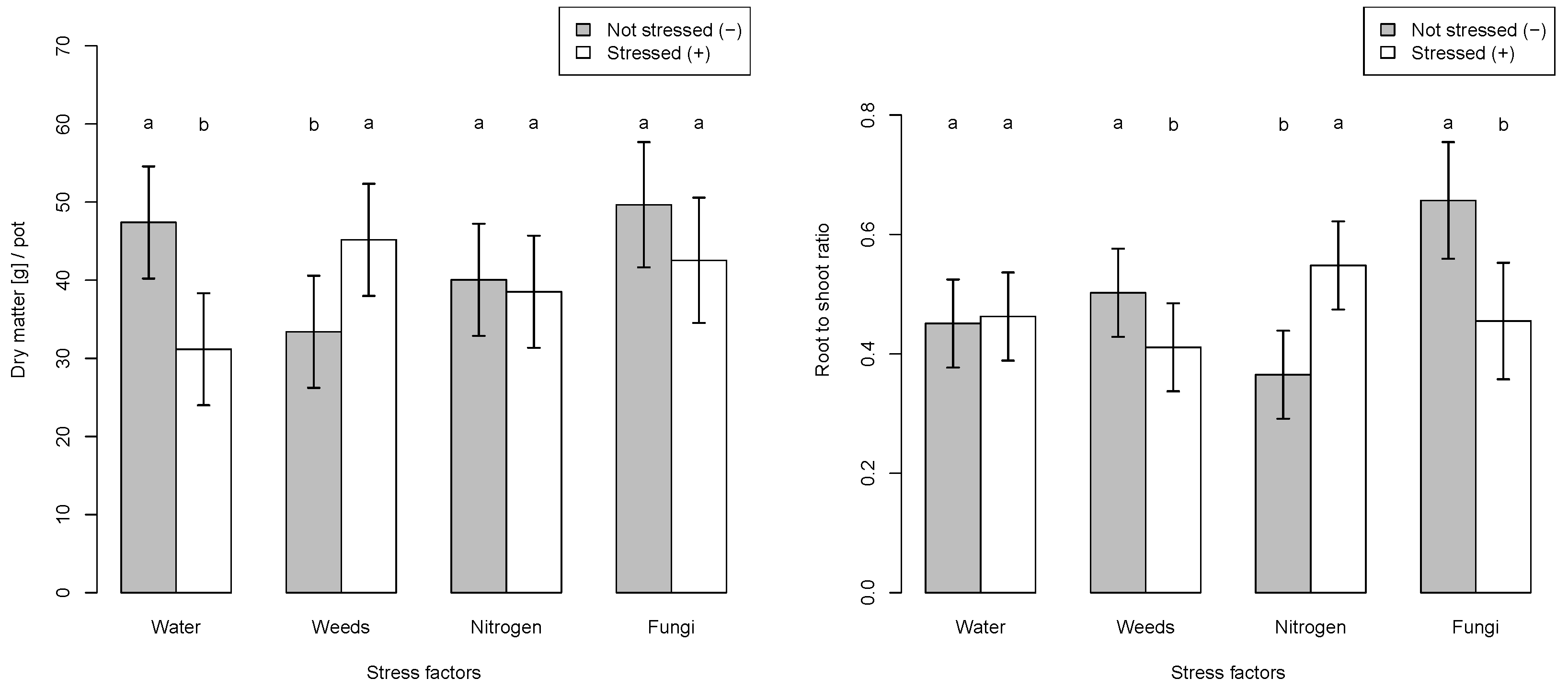
The biomass and the shoot-to-root ratio measurements showed that the stressors affected plant development. Even though the stress factors were there, they were not causing extreme differences between stressed and non-stressed plants. The largest effect was measured for water content on dry matter production, where the dry matter yields in the water stressed pots averaged 29.5% less than that obtained in the non-water-stressed pots. Hence, the data set should be a good starting point for stress recognition.

4.1. Could Nitrogen Deficiency Stress Be Detected by the Sensors?

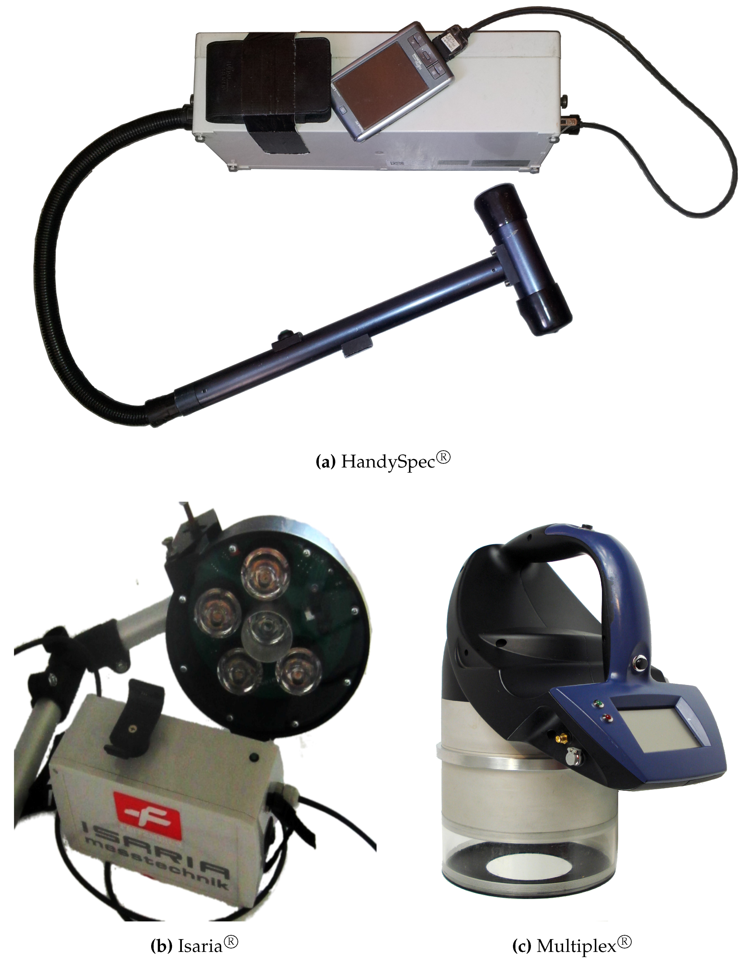
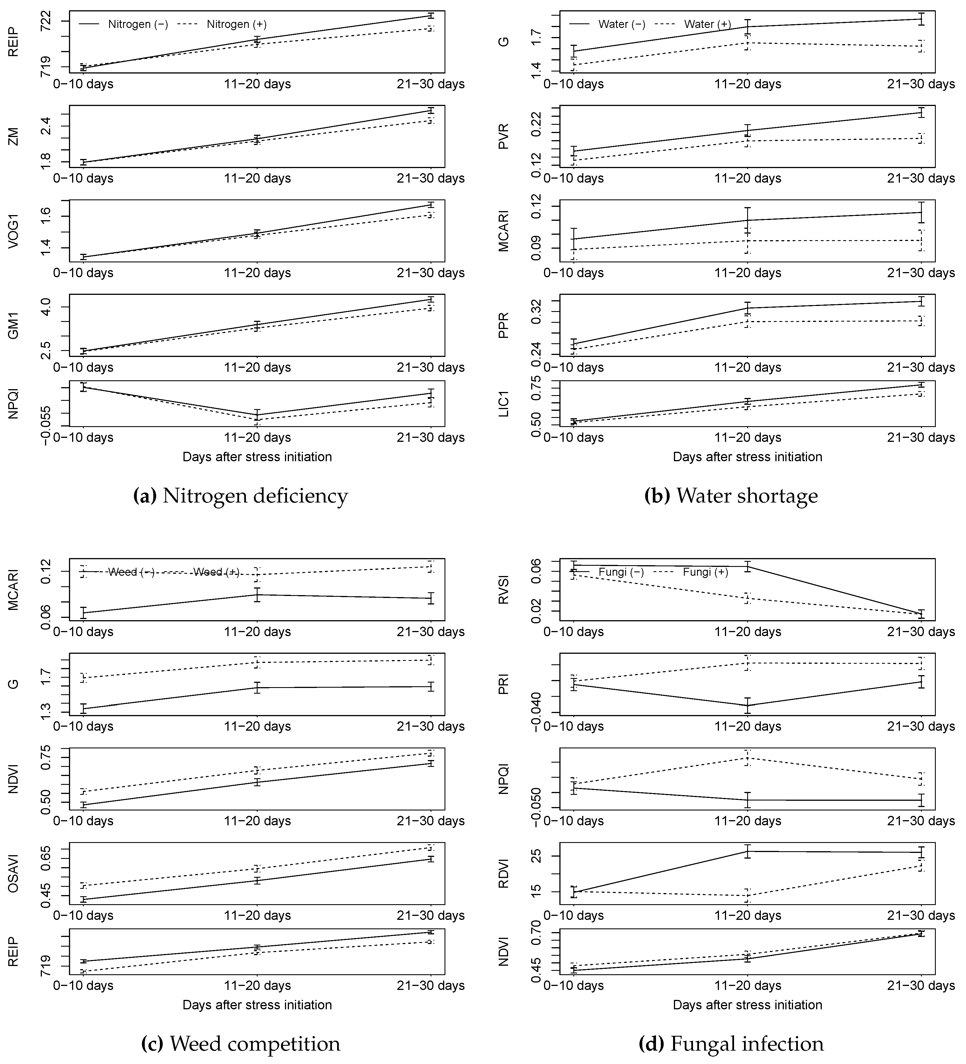
When using the HandySpec indices REIP, ZM, VOG1, and GM1, we were able to discriminate between spring wheat grown with or without sufficient nitrogen supply. REIP was the only index enabling the detection of nitrogen deficiency as early as 11–20 days after onset of stress. It should be noted that all plants had the same nutrient conditions until BBCH 12 (ample resources). The delay in the differentiation between N-stressed and fertilized plants may be attributed to the early growth stages of the plants at time of fertilization, and their relatively limited N demand at this developing stage. As expected, REIP was lower for the stressed than the non-stressed plants. This agrees with the well documented red shift of the REIP due to higher concentrations of chlorophyll, which normally follows increased plant N availability. [16,49,50,51,52,53]. The indices VOG1, ZM and GM1 have also been proven to correlate with chlorophyll content [16,54,55]. Taking into account that VOG and ZM are simple ratios centered around 730 nm (red), both can be considered as gross estimators of the REIP. In contrast, GM1 also involves reflection from the green area (dividing reflectance at 750 nm with that at 550 nm), and has been reported to correlate well with total chlorophyll along with nutrition and fertilization level [8,52,53,56].
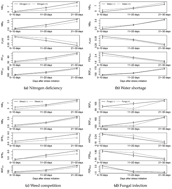
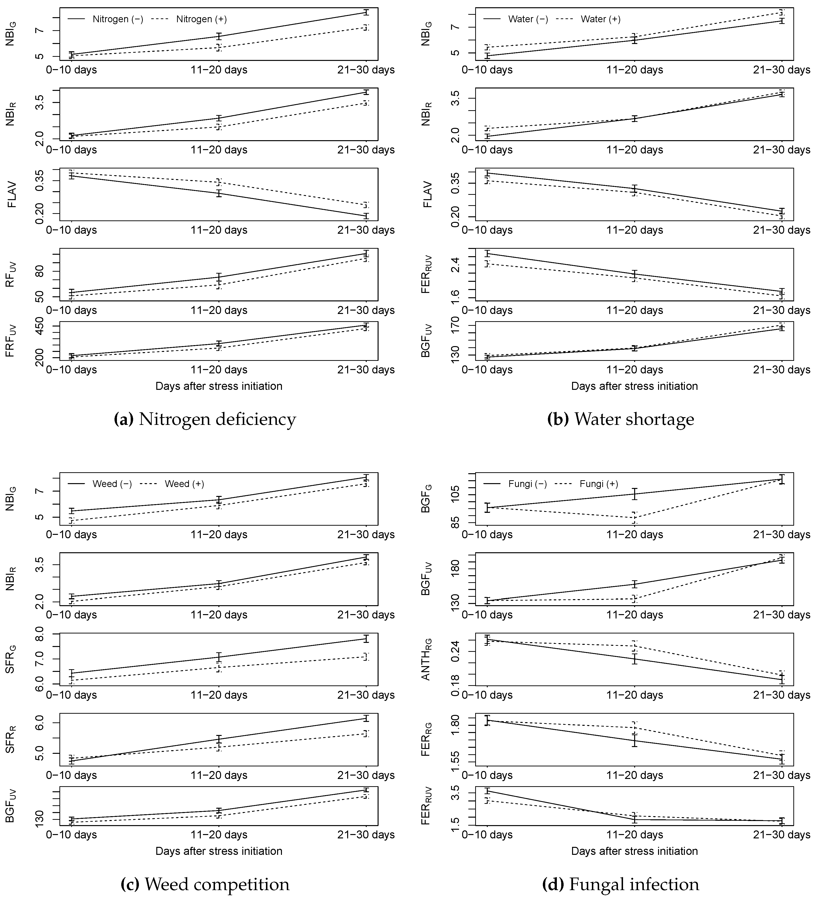
Five of the twelve indices measured with the Multiplex® sensor could be used to detect nitrogen deficiency as early as the 11–20 day period. The indices N B I G and N B I R clearly differentiated between N-stressed and non-stressed plants, giving lower index values for the stressed than the non-stressed plants. Similar findings have also been reported for bermudagras and turfgrasses [57,58]. Longchamps and Khosla [59] were able to distinguish between all their four N-levels in an experiment with maize, using N B I G and N B I R . In our experiment, we also found out that an index related to flavonoids, FLAV, also contained information usable for nitrogen stress detection. In contrast with N B I G and N B I R , FLAV had higher, not lower values for the stressed plants. This agrees well with results from Agati et al. [58]. Several authors have reported that FLAV correlates with the flavonoid levels in fruits [13,60,61,62]. Cartelat et al. [13] found a negative correlation between flavonoid levels and chlorophyll content in wheat. All in all concerning nitrogen deficiency, both the spectrometer and the fluorometer were able to detect nitrogen deficiency. REIP, VOG1, ZM, N B I G , N B I R and FLAV can be used for this identification. On the other hand, the Isaria® sensor did not provide significant data.

4.2. Could Water Stress Be Detected by the Sensors?

Among the five indices presented for HandySpec® capable in detecting shortage in water, PVR and G could detect it already 0–10 DAS. This was well before any visual symptoms of water deprivation occurred. PVR, MCARI and G showed relatively stable values from the 10th DAS and onwards. All the above indices utilize the reflection of 550 nm (green) in their formula. Lin et al. [17] pinpointed a shift of the region around 535–540 nm with the water content of Cinnamomum camphora (Linn.) Seib. Kusnierek and Korsaeth [63] identified the region 560–610 nm as one of three spectral regions in the range 400–950 nm containing significant information related to water status in spring wheat. Thenkabail et al. [8] associates the wavebands around 550 nm with total chlorophyll and biomass, therefore water stress measurements also derive indirectly from chlorophyll measurements. Wang et al. [64] also showed a robust correlation between PPR and chlorophyll concentration. In the current study, NDVI, SAVI, OSAVI, VOG1, LIC1, GM1 and ZM could also be used to differentiate between water deprived and non stressed plants 20–30 DAS. These indices have also previously been associated with water content in plants [9,17,18,19,20]. The correlations between the indices NDVI, SAVI, OSAVI, VOG1, LIC1, GM1 and ZM at one side and plant water status at the other were probably an indirect result, as water deprivation affects other parameters of plant growth, like chlorophyll content and leaf area index, which these indices correlate better with.
Using the Multiplex® device, four indices ( F E R R U V , FLAV, N B I G , and N B I R ) enabled early detection of water shortage. Two of the indices, FLAV and NBI, have previously been associated with water tolerance in wheat [14]. Concerning water stress for both the spectrometer and the fluorometer, the presented approach appears promising. It can be argued that the spectrometer performed better than the fluorometer in this task, since the basic recognition indices in the fluorometer are the same as for nitrogen. PVR and G from the spectrometer can be used for water identification. However, the robustness of all indices related with water should be confirmed by further studies.

4.3. Could Weed Competition Be Detected by the Sensors?

As expected, weed competition was correlated with many indices calculated from the HandySpec® data. As for water shortage, G and other indices correlating with the Leaf Area Index (LAI), like NDVI and OSAVI, could be used to identify weediness from the first days of the experiment and onwards. The stress factor weeds, differed markedly from the other stressors we imposed, as the weed plants were physically present from the first day of measurement. Since the pots occupy a predefined space, the plant biomass and the LAI were thus already higher at the beginning of the measurement period, compared with pots without any weeds planted.
Vegetation Indices like NDVI, REIP, OSAVI, ZM, RDVI and LIC1, contained not only the information needed to separate between pots with or without weeds, but they also showed an increase with time, reflecting the growth in biomass during the experiment (both treatments). Measurements were performed at the early growing stages of the plants (BBCH 12–40). Therefore, crop plants were also rapidly growing, resulting in a continuous increase in e.g., LAI, commonly shown to be positively correlated with NDVI. Indices like PVR and PPR could be used to identify weed presence from days 11–20 and beyond. Since the pot size and volume are finite, this result might be an indirect result from water stress, due to assumedly higher transpiration from pots with weed and wheat plants than from pots with wheat plants alone.
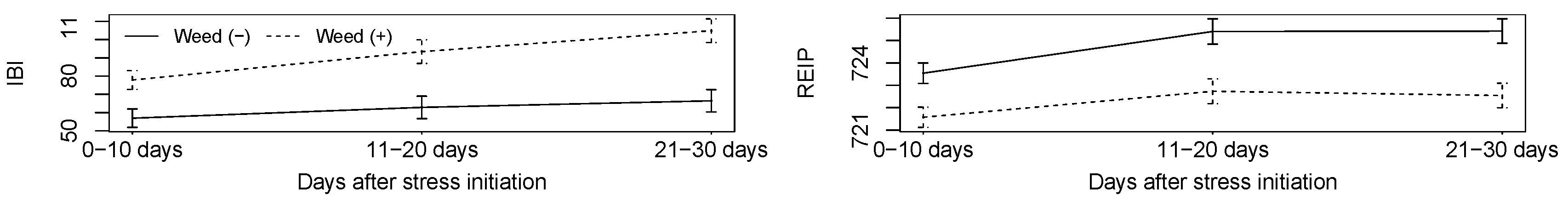
Weed treatments could be separated by means of the indices REIP and IBI as obtained by the active spectrometer Isaria®. The REIP as calculated from the Isaria sensor gave higher values than the REIP calculated by the Handyspec®-sensor. This agrees with the findings of Peteinatos et al. [65]. The Multiplex provided useful data, as four of its output-indices ( B G F U V , S F R G , S F R R and N B I G ) could be used to separate the weed treatments.
All three sensors provided information for weed identification. HandySpec® and Isaria® provided bigger differences faster than the fluorometer. It should be noted that the classical method of detecting weeds is by combining high-density RGB-images and image analysis. Such an approach is, however, less useful for detecting the other stressors of interest in the current study. Moreover, image-based weed detection is normally performed with the weed plants at a very early development stage, mainly to reflect the timing of herbicide application in practice. In this study, we focused on the combined effect of more stressors, and thus selected sensors, which had a potential for identifying more than one stressor. Therefore, from our perspective, indices MCARI, G, NDVI and OSAVI were able to perform this task along with S F R G and S F R R .

4.4. Could Fungal Infection Be Detected by Sensors?

Two indices calculated from data obtained by the HandySpec® could be used to identify infection by powdery mildew (B. graminis) as soon as 0–10 DAS, NDVI and RVSI, the latter also 11–20 DAS. This clearly suggests that RVSI is suitable for early, pre-visual, detection of powdery mildew in wheat. Bauriegel et al. [11] and Bauriegel and Herppich [27] identified the spectra around 550–560 nm, and 665–675 nm as important for identifying Fusarium infection in wheat, but they could not find any significant results with NDVI, G and LIC1. Two of the above indices, MCARI and RDVI, use at least one of the above two spectral ranges in their calculations. Time-wise, the results showed an interesting point. A series of four indices could discriminate between infested and non-infested in the second time period. These could also provide indices which enabled a differentiation in the third period, but differences became smaller. Zhang et al. [26] made a similar observation when investigating yellow rust infection over 17 days (four measurements at 216 till 233 days after sowing) in wheat with NDVI, PRI, RVSI and MCARI. Their results also showed the highest correlations at the second measuring date (225 days after sowing), whereas five days later only PRI was correlated with yellow rust infection. We cannot explain this phenomenon based on the current data, but this should be investigated in more detail, since this may be a potential important issue related to pre-symptomatic fungi detection. Indices like PRI and MCARI that identified water stress and NDVI and MCARI that identified weed presence, were also able to identify fungi infection. Zhang et al. [26] reported similar results for PRI. The fact that all types of spectral indices correlated with presence of fungi can be attributed to the result that fungi infected plants had a reduced growth dynamic, a lower total biomass and LAI.
Multiplex® could also differentiate between fungi infected and non-infected plants. Blue-Green fluorescence under green or ultraviolet excitation ( B G F G and B G F U V ) and indices relative to Ferodoxines and Anthocyanins could be used to identify the fungal infection. F E R R G and A N T H R G seemed sensitive only on fungal infection. This can make them an indicator for B. graminis. Latouche et al. [66] used Multiplex® to successfully identify Plasmopara viticola in vineyards, yet the sensor setup was modified. Time-wise, B G F G , B G F U V , F E R R G and A N T H R G were able to identify the fungal infection in the second 10-day period. The result seems similar to the result of the HandySpec® sensor. Only F E R R U V was able to identify the fungal infection in the first 10-day period. However, it identified it only in the first 10-day period and the results, even if it is not statistically significant, were reversed in the second 10-day period. Therefore, more experimentation is needed to see if this index can be used as a tool to identify B. graminis. Concerning fungal infection, the small time windows that it can be measured in, makes it challenging to be identified by both spectral and fluorescence data.

4.5. Could Combinations of Stressors Be Detected by Sensors?

A lot of indices both from the HandySpec® and the Multiplex
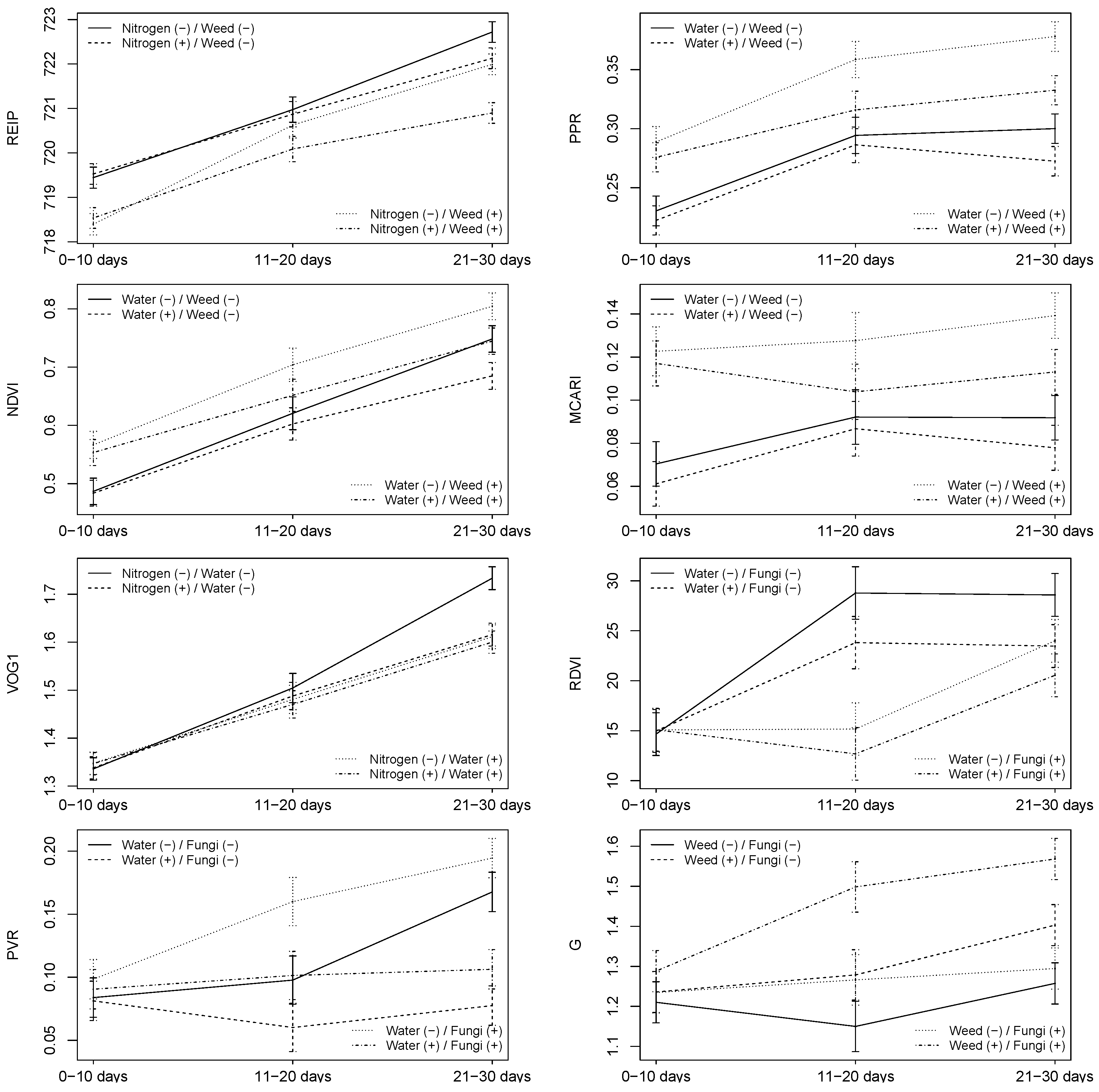
® sensor showed correlations with more than one stress factor. In the combination of stress factors, if we take into account the different way that each index reacts to each stressor, the increase through time for most of the indexes and the different rate of increase per stressor, identifying combinations of stressors with the same index can be quite challenging. For example, REIP as presented in Figure 3c in the first 10-day period can clearly differentiate weedy from weed free pots, but could not differentiate per weed group the nitrogen stress. As days passed by, the non-nitrogen stressed plants increased in value at a higher rate than the non-stressed plants. In the third 10-day period, there was a clear distinction, between the control and the stressed pots. The pots containing only one of the two stressors could not be differentiated from each other. Similar results can be noted for RDVI where, in the second 10-day period, it can clearly differentiate between all four water shortage and fungal infection combinations. On 21–30 DAS, only three groups are clearly distinguishable (control, combinations, one stressor). For weed presence and fungal infection, G presents the aforementioned three groups on the 10–20 DAS, but in the third 10-day period, fungal infection cannot be differentiated on the weed free pots. Weedy pots could clearly be differentiated from weed free and in their case fungal infection could also be pinpointed. On the other hand, VOG1 can only differentiate the control from the other three treatments in the third 10-day period. Zhang et al. [26] also pinpointed the difficulty of identifying more than one stress factor with the same index.
In cases where the results of the two stressors are heading in the opposite direction, identifying the existence of one stressor or the other can be easy. We can see this in PPR, NDVI and MCARI for separating water shortage and weed presence and in PVR for the identification of weed presence and fungal infection from 10–20 DAS onwards. On the other hand, identification between the control and the combinations of the two stressors is harder. The ability to identify the control from the combination of two stressors relies only on the condition, if the results on the index for one stressor are higher than the other. NDVI is not able to perform this, while the rest of the aforementioned indices can perform this separation in the third 10-day period.
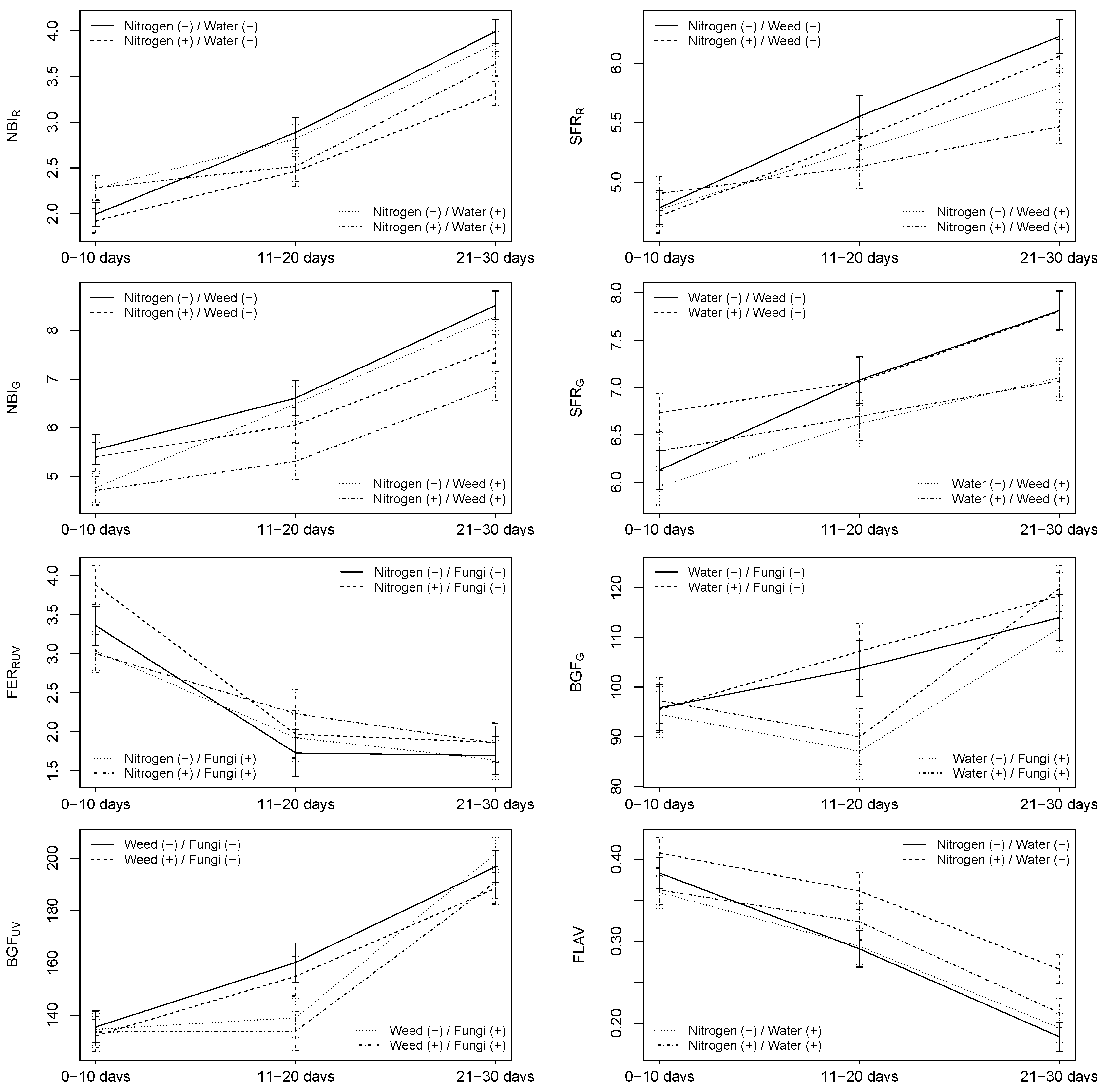
Combination of more than one stressor with the aid of the same index seems harder for the Multiplex® sensor. N B I R can separate nitrogen deficiency in the combination with water shortage from the second 10-day period onwards. N B I G can do the same for the combination of nitrogen deficiency and weed presence. For both indices, only the pots having nitrogen deficiency could differentiate the second stressor (water deficiency and weed presence) in the third 10-day period. B G F G and B G F U V could differentiate fungal infection in the second 10-day period in the combination of water shortage and weed presence, respectively. In the third 10-day period, B G F G could separate only water shortage and B G F U V only weeds. Identification of both stressors was not performed simultaneously but in different time periods. That pinpoints the constraints of creating a robust stress identification based on sensor values. Depending on the circumstances, a similar result could be attributed to one or more different stressors. A similar example can be S F R G which can differentiate water stress in weed free pots in the first 10-day period. However, from the 11–20 DAS onwards, the differentiation performed is only weedy and weed free pots regardless of the water stress. Concerning interaction of more than two factors, no significant results were identified.

5. Conclusions

Water deficiency and fungal infection could be detected pre-symptomatic, i.e., 0–10 days after stress induction (DAS), with one or more of the sensors tested. The presence or absence of weeds could also be identified using the same sensors (present during the entire experiment).
Nitrogen shortage could be detected 10–20 DAS by the index REIP (Red Edge Inflection Point) measured with HandySpec® and several indices based on Multiplex. The lack in detection of nitrogen shortage earlier could be attributed to the early growth stage (BBCH 12–14) and hence the limited nitrogen needs. Water deprivation in spring wheat could be detected as early as 0–10 days after stress induction (DAS) by the Photosynthetic Vigor Ratio (PVR; 550 nm − 650 nm/550 nm + 650 nm), the Plant Pigment Ratio (PPR; 550 nm − 450 nm/550 nm + 450 nm) and Greenness (G; 554 nm/677 nm) from the HandySpec® spectrometer and several indices based on the Multiplex® fluorometer. Weediness (Sinapis alba) could be detected from 0–10 DAS and onwards by indices measured by all three sensors, including REIP and biomass index (IBI) from the Isaria sensor. Fungal infection in spring wheat (Blumeria graminis f. sp. tritici) could be detected from 0–10 DAS by Red-edge Vegetation Stress Index (RVSI; (714 nm + 752 nm/2) − 733), Photochemical Reflectance Index (PRI; 531 nm − 570 nm/531 nm + 570 nm) and Normalized Phaeophytinization Index (NPQI; 415 nm − 435 nm/415 nm + 435 nm) measured with HandySpec® and by the ratio F E R R G (Fluorescence Excitation Ratio; Red/Green excitiation) measured with Multiplex®. One of the main findings of this study was that the results both from spectral and from fluorescence data varied more due to the plant development rather than the presence or absence of a stress factor. In a lot of cases, where values were attributed to stressed plants at the early stages, ten or twenty days later the same values are then attributed to the non stressed plants. The study shows that it is possible to distinguish between a stressed plant and an unstressed control plant at the same growth stage, but we cannot pinpoint a general threshold value to use for discrimination regardless of the plant development stage. This hinders the stress identification process. More work needs to be done in order to model how the spectral indices change with the growth stage of the plants. In some cases, interactions of more than one stress factor could be viewed with the aid of the same index, yet these results are more complicated to interpret. Interactions with more than two stress factors could not present any significant results. None of the indices showed a significant three-way interaction.

Acknowledgments

The authors would like to thank the Alexander S. Onassis Public Benefit Foundation, the Carl-Zeiss foundation, and The Research Council of Norway (program BIONÆR, project MULTISENS, project number 207829) for funding. We would like to thank Victor Rueda-Ayala for his valuable ideas to set up the experiment and analyze the data. We would also like to thank Christoph Kunz, Manuel Geisser, Julian Börner and Yuxuan Wang for their help in the measurements.

Author Contributions

All authors contributed extensively to this work. Gerassimos Peteinatos organized the execution of the experimental setup, analysed the data, evaluated the results and drafted the manuscript. Audun Korsaeth helped in the design of the experimental setup, data analysis and evaluation and aided the drafting of the manuscript. Therese W. Berge participated in the draft of the manuscript and its revisions. Roland Gerhards helped in the design of the experiment, the drafting and revision of the paper.

Conflicts of Interest

The authors declare no conflicts of interest.

References

  1. Farooq, M.; Hussain, M.; Wahid, A.; Siddique, K.H.M. Drought Stress in Plants: An Overview. In Plant Responses to Drought Stress; Springer: Berlin, Germany; Heidelberg, Germany, 2012; pp. 1–33. [Google Scholar]
  2. Oerke, E. Crop losses to pests. J. Agric. Sci. 2006, 144, 31–43. [Google Scholar] [CrossRef]
  3. Zhao, G.; Miao, Y.; Wang, H.; Su, M.; Fan, M.; Zhang, F.; Jiang, R.; Zhang, Z.; Liu, C.; Liu, P.; et al. A preliminary precision rice management system for increasing both grain yield and nitrogen use efficiency. Field Crops Res. 2013, 154, 23–30. [Google Scholar] [CrossRef]
  4. San Martín, C.; Andújar, D.; Fernández-Quintanilla, C.; Dorado, J. Spatial distribution patterns of weed communities in corn fields of Central Spain. Weed Sci. 2015, 63, 936–945. [Google Scholar] [CrossRef]
  5. Tremblay, N.; Wang, Z.; Cerovic, Z.G. Sensing crop nitrogen status with fluorescence indicators. A review. Agron. Sustain. Dev. 2011, 32, 451–464. [Google Scholar] [CrossRef]
  6. Peteinatos, G.G.; Weis, M.; Andújar, D.; Rueda Ayala, V.; Gerhards, R. Potential use of ground-based sensor technologies for weed detection. Pest Manag. Sci. 2014, 70, 190–199. [Google Scholar] [CrossRef] [PubMed]
  7. Govender, M.; Govender, P.J.; Weiersbye, I.M.; Witkowski, E.T.F.; Ahmed, F. Review of commonly used remote sensing and ground-based technologies to measure plant water stress. Water SA 2009, 35, 741–752. [Google Scholar] [CrossRef]
  8. Thenkabail, P.S.; Lyon, J.G.; Huete, A. (Eds.) Hyperspectral Remote Sensing of Vegetation; Taylor & Francis, CRC Press: Boca Raton, FL, USA, 2011.
  9. Tilling, A.K.; O’Leary, G.J.; Ferwerda, J.G.; Jones, S.D.; Fitzgerald, G.J.; Rodriguez, D.; Belford, R. Remote sensing of nitrogen and water stress in wheat. Field Crops Res. 2007, 104, 77–85. [Google Scholar] [CrossRef]
  10. Li, F.; Miao, Y.; Hennig, S.D.; Gnyp, M.L.; Chen, X.; Jia, L.; Bareth, G. Evaluating hyperspectral vegetation indices for estimating nitrogen concentration of winter wheat at different growth stages. Precis. Agric. 2010, 11, 335–357. [Google Scholar] [CrossRef]
  11. Bauriegel, E.; Giebel, A.; Herppich, W.B. Hyperspectral and chlorophyll fluorescence imaging to analyze the impact of Fusarium culmorum on the photosynthetic integrity of infected wheat ears. Sensors 2011, 11, 3765–3779. [Google Scholar] [CrossRef] [PubMed]
  12. Backoulou, G.F.; Elliott, N.C.; Giles, K.L.; Mirik, M. Processed multispectral imagery differentiates wheat crop stress caused by greenbug from other causes. Comput. Electron. Agric. 2015, 115, 34–39. [Google Scholar] [CrossRef]
  13. Cartelat, A.; Cerovic, Z.; Goulas, Y.; Meyer, S.; Lelarge, C.; Prioul, J.L.; Barbottin, A.; Jeuffroy, M.H.; Gate, P.; Agati, G.; et al. Optically assessed contents of leaf polyphenolics and chlorophyll as indicators of nitrogen deficiency in wheat (Triticum aestivum L.). Field Crops Res. 2005, 91, 35–49. [Google Scholar] [CrossRef]
  14. Bürling, K.Z.C.; Cornic, G.; Ducruet, J.; Noga, G.; Hunsche, M. Fluorescence-based sensing of drought-induced stress in the vegetative phase of four contrasting wheat genotypes. Environ. Exp. Bot. 2013, 89, 51–59. [Google Scholar] [CrossRef]
  15. Strachan, I.B.; Pattey, E.; Boisvert, J.B. Impact of nitrogen and environmental conditions on corn as detected by hyperspectral reflectance. Remote Sens. Environ. 2002, 80, 213–224. [Google Scholar] [CrossRef]
  16. Vogelmann, J.E.; Rock, B.N.; Moss, D.M. Red edge spectral measurements from sugar maple leaves. Int. J. Remote Sens. 1993, 14, 1563–1575. [Google Scholar] [CrossRef]
  17. Lin, C.; Popescu, S.C.; Huang, S.C.; Chang, P.T.; Wen, H.L. A novel reflectance-based model for evaluating chlorophyll concentrations of fresh and water-stressed leaves. Biogeosciences 2015, 12, 49–66. [Google Scholar] [CrossRef]
  18. Suárez, L.; Zarco-Tejada, P.; Sepulcre-Cantó, G.; Pérez-Priego, O.; Miller, J.; Jiménez-Muñoz, J.; Sobrino, J. Assessing canopy PRI for water stress detection with diurnal airborne imagery. Remote Sens. Environ. 2008, 112, 560–575. [Google Scholar] [CrossRef]
  19. Zarco-Tejada, P.; González-Dugo, V.; Berni, J. Fluorescence, temperature and narrow-band indices acquired from a UAV platform for water stress detection using a micro-hyperspectral imager and a thermal camera. Remote Sens. Environ. 2012, 117, 322–337. [Google Scholar] [CrossRef]
  20. Metternicht, G. Vegetation indices derived from high-resolution airborne videography for precision crop management. Int. J. Remote Sens. 2003, 24, 2855–2877. [Google Scholar] [CrossRef]
  21. Vrindts, E.; Baerdemaeker, J.D.; Ramon, H. Weed Detection using canopy reflection. Precis. Agric. 2002, 3, 63–80. [Google Scholar] [CrossRef]
  22. Haboudane, D.; Miller, J.R.; Pattey, E.; Zarco-Tejada, P.J.; Strachan, I.B. Hyperspectral vegetation indices and novel algorithms for predicting green LAI of crop canopies: Modeling and validation in the context of precision agriculture. Remote Sens. Environ. 2004, 90, 337–352. [Google Scholar] [CrossRef]
  23. Longchamps, L.; Panneton, B.; Samson, G.; Leroux, G.; Thériault, R. Discrimination of corn, grasses and dicot weeds by their UV-induced fluorescence spectral signature. Precis. Agric. 2010, 11, 181–197. [Google Scholar] [CrossRef]
  24. Tyystjärvi, E.; Norremark, M.; Mattila, H.; Keranen, M.; Hakala-Yatkin, M.; Ottosen, C.; Rosenqvist, E. Automatic identification of crop and weed species with chlorophyll fluorescence induction curves. Precis. Agric. 2011, 12, 546–563. [Google Scholar] [CrossRef]
  25. Rumpf, T.; Mahlein, A.K.; Steiner, U.; Oerke, E.C.; Dehne, H.W.; Plümer, L. Early detection and classification of plant diseases with Support Vector Machines based on hyperspectral reflectance. Comput. Electron. Agric. 2010, 74, 91–99. [Google Scholar] [CrossRef]
  26. Zhang, J.; Pu, R.; Huang, W.; Yuan, L.; Luo, J.; Wang, J. Using in-situ hyperspectral data for detecting and discriminating yellow rust disease from nutrient stresses. Field Crops Res. 2012. [Google Scholar] [CrossRef]
  27. Bauriegel, E.; Herppich, W.B. Hyperspectral and chlorophyll fluorescence imaging for early detection of plant diseases, with special reference to Fusarium spec. infections on wheat. Agriculture 2014, 4, 32–57. [Google Scholar] [CrossRef]
  28. Calderón, R.; Navas-Cortés, J.A.; Zarco-Tejada, P.J. Early detection and quantification of verticillium wilt in olive using hyperspectral and thermal imagery over large areas. Remote Sens. 2015, 7, 5584–5610. [Google Scholar] [CrossRef]
  29. Karimi, Y.; Prasher, O.S.; Patel, M.R.; Kim, H.S. Application of support vector machine technology for weed and nitrogen stress detection in corn. Comput. Electron. Agric. 2006, 51, 99–109. [Google Scholar] [CrossRef]
  30. Mitscherlich, E.A. Das Gesetz des Miniraums und das Gesetz des abhnehlmenden Bodenertrags. Land. Jahrb 1909, 38, 5371–5552. [Google Scholar]
  31. Hess, M.; Barralis, G.; Bleiholder, H.; Buhr, L.; Eggers, T.; Hack, H.; Stauss, R. Use of the extended BBCH scale—General for the descriptions of the growth stages of mono and dicotyledonous weed species. Weed Res. 1997, 37, 433–441. [Google Scholar] [CrossRef]
  32. Rouse, J.W.; Haas, R.H.; Schell, J.A.; Deering, D.W.; Harlan, J.C. Monitoring the Vernal Advancement and Retrogradation (Greenwave Effect) of Natural Vegetation; Texas A & M University, Remote Sensing Center: College Station, TX, USA, 1974. [Google Scholar]
  33. Rondeaux, G.; Steven, M.; Baret, F. Optimization of soil-adjusted vegetation indices. Remote Sens. Environ. 1996, 55, 95–107. [Google Scholar] [CrossRef]
  34. Roujean, J.L.; Breon, F.M. Estimation PAR absorbed by vegetation from bi-directional reflectance measurements. Remote Sens. Environ. 1995, 51, 375–384. [Google Scholar] [CrossRef]
  35. Guyot, G.; Baret, F.; Major, D.J. High spectral resolution: Determination of spectral shifts between the red and infrared. Int. Arch. Photogram. Remote Sens. 1988, 11, 750–760. [Google Scholar]
  36. Zarco-Tejada, P.; Berjón, A.; López-Lozano, R.; Miller, J.; Martín, P.; Cachorro, V.; González, M.; de Frutos, A. Assessing vineyard condition with hyperspectral indices: Leaf and canopy reflectance simulation in a row-structured discontinuous canopy. Remote Sens. Environ. 2005, 99, 271–287. [Google Scholar] [CrossRef]
  37. Daughtry, C.S.; Walthall, C.L.; Kim, M.S.; Brown de Colstoun, E.; McMurtrey, J.E. Estimating corn leaf chlorophyll concentration from leaf and canopy reflectance. Remote Sens. Environ. 2000, 74, 229–239. [Google Scholar] [CrossRef]
  38. Barnes, J.; Balaguer, L.; Manrique, E.; Elvira, S.; Davison, A. A reappraisal of the use of DMSO for the extraction and determination of chlorophylls a and b in lichens and higher plants. Environ. Exp. Bot. 1992, 32, 85–100. [Google Scholar] [CrossRef]
  39. Gitelson, A.A.; Merzlyak, M.N. Remote estimation of chlorophyll content in higher plant leaves. Int. J. Remote Sens. 1997, 18, 2691–2697. [Google Scholar] [CrossRef]
  40. Lichtenthaler, H.K. Vegetation stress: An introduction to the stress concept in plants. J. Plant Physiol. 1996, 148, 4–14. [Google Scholar] [CrossRef]
  41. Zarco-Tejada, P.J.; Miller, J.R.; Noland, T.L.; Mohammed, G.H.; Sampson, P.H. Scaling-up and model inversion methods with narrow-band optical indices for chlorophyll content estimation in closed forest canopies with hyperspectral data. IEEE Trans. Geosci. Remote Sen. 2001, 39, 1491–1507. [Google Scholar] [CrossRef]
  42. Gamon, J.A.; Peñuelas, J.; Field, C.B. A narrow-waveband spectral index that tracks diurnal changes in photosynthetic efficiency. Remote Sens. Environ. 1992, 41, 35–44. [Google Scholar] [CrossRef]
  43. Carter, G.A. Ratios of leaf reflectances in narrow wavebands as indicators of plant stress. Int. J. Remote Sens. 1994, 15, 697–703. [Google Scholar] [CrossRef]
  44. Merton, R. Monitoring Community Hysteresis Using Spectral Shift Analysis and the Red-Edge Vegetation Stress Index; Jet Propulsion Laboratory: Pasadena, CA, USA, 1998. [Google Scholar]
  45. FORCE-A. Users Guide, Multiplex 3, Hand-Held Multi-Parameter Optical Sensor; FORCE-A, Centre Universitaire Paris-Sud ORSAY: Cedex, France, 2010. [Google Scholar]
  46. Ghozlen, N.B.; Cerovic, Z.G.; Germain, C.; Toutain, S.; Latouche, G. Non-destructive optical monitoring of grape maturation by proximal sensing. Sensors 2010, 10, 10040–10068. [Google Scholar] [CrossRef] [PubMed]
  47. Cerovic, Z.; Moise, N.; Agati, G.; Latouche, G.; Ghozlen, N.B.; Meyer, S. New portable optical sensors for the assessment of winegrape phenolic maturity based on berry fluorescence. J. Food Compos. Anal. 2008, 21, 650–654. [Google Scholar] [CrossRef]
  48. R Development Core Team. R: A Language and Environment for Statistical Computing; R Foundation for Statistical Computing: Vienna, Austria, 2008. [Google Scholar]
  49. Boochs, F.; Kupfer, G.; Dockter, K.; Kühbauch, W. Shape of the red edge as vitality indicator for plants. Int. J. Remote Sens. 1990, 11, 1741–1753. [Google Scholar] [CrossRef]
  50. Miller, J.R.; Hare, E.W.; Wu, J. Quantitative characterization of the vegetation red edge reflectance 1. An inverted-Gaussian reflectance model. Int. J. Remote Sens. 1990, 11, 1755–1773. [Google Scholar] [CrossRef]
  51. Belanger, M.; Miller, J.; Boyer, M. Comparative relationships between some red edge parameters and seasonal leaf chlorophyll concentrations. Can. J. Remote Sens. 1995, 21, 16–21. [Google Scholar] [CrossRef]
  52. Zhao, D.; Reddy, K.R.; Kakani, V.G.; Reddy, V. Nitrogen deficiency effects on plant growth, leaf photosynthesis, and hyperspectral reflectance properties of sorghum. Eur. J. Agron. 2005, 22, 399–403. [Google Scholar] [CrossRef]
  53. Corp, L.A.; Middleton, E.M.; Campbell, P.E.; Huemmrich, K.F.; Daughtry, C.S.; Russ, A.; Cheng, Y.B. Spectral indices to monitor nitrogen-driven carbon uptake in field corn. J. Appl. Remote Sens. 2010, 4. [Google Scholar] [CrossRef]
  54. Zarco-Tejada, P.J.; Berjón, A.; Miller, J.R. Stress detection in crops with hyperspectral remote sensing and physical simulation models. In Proceedings of the Airborne Imaging Spectroscopy Workshop, Bruges, Belgium, 8 October 2004.
  55. Zarco-Tejada, P.J.; Miller, J.R.; Harron, J.; Hu, B.; Noland, T.L.; Goel, N.; Mohammed, G.H.; Sampson, P. Needle chlorophyll content estimation through model inversion using hyperspectral data from boreal conifer forest canopies. Remote Sens. Environ. 2004, 89, 189–199. [Google Scholar] [CrossRef]
  56. Campbell, P.E.; Middleton, E.; Corp, L.; Kim, M. Contribution of chlorophyll fluorescence to the apparent vegetation reflectance. Sci. Total Environ. 2008, 404, 433–439. [Google Scholar] [CrossRef] [PubMed]
  57. Agati, G.; Foschi, L.; Grossi, N.; Volterrani, M. In field non-invasive sensing of the nitrogen status in hybrid bermudagrass (Cynodon dactylon × C. transvaalensis Burtt Davy) by a fluorescence-based method. Eur. J. Agron. 2015, 63, 89–96. [Google Scholar] [CrossRef]
  58. Agati, G.; Foschi, L.; Grossi, N.; Guglielminetti, L.; Cerovic, Z.G.; Volterrani, M. Fluorescence-based versus reflectance proximal sensing of nitrogen content in Paspalum vaginatum and Zoysia matrella turfgrasses. Eur. J. Agron. 2013, 45, 39–51. [Google Scholar] [CrossRef]
  59. Longchamps, L.; Khosla, R. Early detection of nitrogen variability in maize using fluorescence. Agron. J. 2014, 106, 511–518. [Google Scholar] [CrossRef]
  60. Cerovic, Z.; Ounis, A.; Cartelat, A.; Latouche, G.; Goulas, Y.; Meyer, S.; Moya, I. The use of chlorophyll fluorescence excitation spectra for the nondestructive in situ assessment of UV-absorbing compounds in leaves. Plant Cell Environ. 2002, 25, 1663–1676. [Google Scholar] [CrossRef]
  61. Bilger, W.; Veit, M.; Schreiber, L.; Schreiber, U. Measurement of leaf epidermal transmittance of UV radiation by chlorophyll fluorescence. Physiol. Plant 1997, 101, 754–763. [Google Scholar] [CrossRef]
  62. Bilger, W.; Johnsen, T.; Schreiber, U. UV-excited chlorophyll fluorescence as a tool for the assessment of UV-protection by the epidermis of plants. J. Exp. Bot. 2001, 52, 2007–2014. [Google Scholar] [CrossRef] [PubMed]
  63. Kusnierek, K.; Korsaeth, A. Simultaneous identification of spring wheat nitrogen and water status using visible and near infrared spectra and powered partial least squares regression. Comput. Electron. Agric. 2015, 117, 200–213. [Google Scholar] [CrossRef]
  64. Wang, C.; Qi, J.; Moran, S.; Marsett, R. Soil moisture estimation in a semiarid rangeland using ERS-2 and TM imagery. Remote Sens. Environ. 2004, 90, 178–189. [Google Scholar] [CrossRef]
  65. Peteinatos, G.G.; Keller, M.; Weis, M.; Gerhards, R. Comparison of Isaria Sensor with a Typical Spectrometer in a Series of Diverse Conditions; Edicions de la Universitat de Lleida: Lleida, Spain, 2013; pp. 32–33. [Google Scholar]
  66. Latouche, G.; Debord, C.; Raynal, M.; Milhade, C.; Cerovic, Z.G. First detection of the presence of naturally occurring grapevine downy mildew in the field by a fluorescence-based method. Photochem. Photobiol. Sci. 2015, 14, 1807–1813. [Google Scholar] [CrossRef] [PubMed]
Figure 1. Sensors used in the current experiment.
Agriculture 06 00024 g001
Figure 2. Mean values with their upper and lower confidence intervals of the total (including weeds) below and aboveground biomass and the root to shoot ratio of spring wheat at the end of the experiment (BBCH 40 = 30 days after onset of stress). Different letters indicate significant differences within each category (Tukey’s HSD test).
Agriculture 06 00024 g002
Figure 3. Ten day mean values of spectral indices derived by the HandySpec® sensor. The error bars demonstrate their upper and lower 95% confidence intervals (Tukey’s HSD). The most important indices per stress are shown, separated into three periods: 0–10, 11–20 and 21–30 days after stress induction. ’−’ indicates absence of stress, ’+’ indicates presence of stress.
Agriculture 06 00024 g003
Figure 4. Ten day mean values of spectral indices derived by the Isaria® sensor. The error bars demonstrate their upper and lower 95% confidence intervals (Tukey HSD p = 0.05). The most important indices per stress are shown, separated into three periods: 0–10, 11–20 and 21–30 days after stress induction. ’−’ indicates absence of stress, ’+’ indicates presence of stress.
Agriculture 06 00024 g004
Figure 5. Ten day mean values of spectral indices derived by the Multiplex® sensor. The error bars demonstrate their upper and lower 95% confidence intervals (Tukey’s HSD). The most important indices per stress are shown, separated into three periods: 0–10, 11–20 and 21–30 days after stress induction. ’−’ indicates absence of stress, ’+’ indicates presence of stress.
Agriculture 06 00024 g005
Figure 6. Ten day mean values of spectral indices derived by the HandySpec® sensor. The error bars demonstrate their upper and lower 95% confidence intervals (Tukey HSD). The most important interactions per combination of two stressors are showed, separated into three periods: 0–10, 11–20 and 21–30 days after stress induction. ’−’ indicates absence of stress, ’+’ indicates presence of stress.
Agriculture 06 00024 g006
Figure 7. Ten day mean values of spectral indices derived by the Multiplex® sensor. The error bars demonstrate their upper and lower 95% confidence intervals (Tukey’s HSD). The most important interactions per combination of two stressors are showed, separated into three periods: 0–10, 11–20 and 21–30 days after stress induction. ’−’ indicates absence of stress, ’+’ indicates presence of stress.
Agriculture 06 00024 g007
Table 1. All 16 treatment combinations, with “+” indicating presence of stress, while “−” represents absence of stress.
Treatment12345678910111213141516
Fungi++++++++
Water++++++++
Nitrogen++++++++
Weeds++++++++
Table 2. Overview of the spectral indices and fluorescence parameters measured with the 3 sensors (HandySpec® Field sensor, Multiplex®, Isaria®) used in this study.
Index ReferenceExplanationFormula
Structural indices(HandySpec®)
NDVI [32]Normalized Difference Vegetation Index R 780 R 670 R 780 + R 670
OSAVI [33]Optimized Soil-Adjusted Vegetation Index ( 1 + 0.16 ) R 800 R 670 R 800 + R 670 + 0 . 16
RDVI [34]Renormalized Difference Vegetation Index R 800 R 670 R 800 + R 670
Red Edge Inflection Point(HandySpec® & Isaria®)
REIP [35]Red Edge Inflection Point 700 + 40 ( R 670 + R 780 2 ) R 700 R 740 R 700
Chlorophyll indices(HandySpec®)
G [36]Greenness Index R 554 R 677
MCARI [37]Modified Chlorophyll Absorption in Reflectance Index ( ( R 700 R 670 ) 0.2 ( R 700 R 550 ) ) ( R 700 R 670 )
NPQI [38]Normalized Phaeophytinization Index R 415 R 435 R 415 + R 435
PPR [20]Plant Pigment Ratio R 550 R 450 R 550 + R 450
PVR [20]Photosynthetic Vigor Ratio R 550 R 650 R 550 + R 650
VOG1 [16]Simple Ratio 740/720 R 740 R 720
GM1 [39]Simple Ratio 750/550 R 750 R 550
LIC1 [40]Lichtenthaler Index 1 R 800 R 680 R 800 + R 680
ZM [41]Zarco-Tejada & Miller R 750 R 710
Stress–Pigment indices(HandySpec®)
PRI [42]Photochemical Reflectance Index R 531 R 570 R 531 + R 570
CTR1 [43]Simple Ratio 695/420 R 695 R 420
RVSI [44]Red-edge Vegetation Stress Index R 714 + R 752 2 R 733
Fluorescence indices(Multiplex®)
ANTH [45]Anthocyanins l o g ( F E R R G )
RFR [45]Red Fluorescence (Red Excitation)
FRFUV [45]Infra-red Fluorescence (UV Excitation)
BGFG [45]Blue Green Fluorescence (Green Excitation)
BGFUV [45]Blue Green Fluorescence (UV Excitation)
FERRUV [45]Fluorescence Excitation Ratio (Red & UV Excitation) F R F R F R F U V
FERRG [45]Fluorescence Excitation Ratio (Red & Green Excitation) F R F R F R F G
FLAV [45]Flavonoids l o g ( F E R R U V )
NBIG [45]Nitrogen Balance Index F R F U V R F G
NBIR [45]Nitrogen Balance Index F R F U V R F R
SFRG [45]Simple Fluorescence Ratio (Green Excitation) F R F G R F G
SFRR [45]Simple Fluorescence Ratio (Red Excitation) F R F R R F R
Table 3. Technical characteristics of the senors used in this study.
HandySpec®Isaria®Multiplex®
TypeSpectrometerSpectrometerFluorometer
Has IlluminationNoYesYes
Needs CalibrationYesNoNo
Plant-Sensor Distance (cm) 55 ± 5 6010
Field of View (cm2)20070050
Table 4. Mean values of spectral indices for the main effects derived by the HandySpec® sensor. ’−’ indicates the absence of stress and ’+’ indicates its presence. The significance level is indicated as *** for p < 0.001; ** for p < 0.01; * for p < 0.05, and NS for non-significant differences.
IndexNitrogen DeficiencyWater ShortageWeed CompetitionFungal Infection
+Sign+Sign+Sign+Sign
REIP721720***720721*721720***722721***
NDVI0.640.63NS0.650.62***0.600.67***0.560.58**
PVR0.190.18NS0.200.17***0.150.22***0.100.12***
OSAVI0.580.56NS0.580.56**0.540.60***0.520.51NS
MCARI0.110.11NS0.120.10***0.080.14***0.060.05***
RVSI0.0300.032NS0.0280.034**0.0340.028***0.0470.036***
RDVI23.522.8NS24.022.3*20.625.7***21.917.5***
G1.681.65NS1.751.58***1.501.83***1.261.36***
ZM2.232.15***2.232.15**2.152.23**2.072.09NS
NPQI−0.043−0.045**−0.045−0.044NS−0.046−0.042***−0.046−0.039***
PRI−0.021−0.024*−0.02−0.025***−0.026−0.019***−0.033−0.027***
CTR11.521.56*1.521.55*1.531.55NS1.511.40***
LIC10.640.63NS0.650.61***0.600.66***0.560.58**
VOG11.511.48**1.501.48**1.481.50NS1.461.47NS
GM13.403.24***3.383.26*3.223.42***2.932.88NS
PPR0.290.30NS0.300.28***0.260.32***0.220.22NS
Table 5. Mean values of spectral indices for the main effects derived by the Isaria® sensor. ’−’ indicates the absence of stress and ’+’ indicates its presence. The significance level is indicated as *** for p < 0.001; ** for p < 0.01; * for p < 0.05, and NS for non-significant differences.
IndexNitrogen DeficiencyWater ShortageWeed CompetitionFungal Infection
+Sign+Sign+Sign+Sign
REIP724723NS723724NS725722***726726NS
IBI79.676.3NS80.875.1NS64.391.6***63.264.5NS
Table 6. Mean values of spectral indices for the main effects derived by the Multiplex® sensor. ’−’ indicates the absence of stress and ’+’ indicates its presence. The significance level is indicated as *** for p < 0.001; ** for p < 0.01; * for p < 0.05, and NS for non-significant differences.
IndexNitrogen DeficiencyWater ShortageWeed CompetitionFungal Infection
+Sign+Sign+Sign+Sign
B G F U V 147146NS146148**150144***162158**
R F U V 80.173.5***76.776.8NS74.778.8*101100NS
F R F U V 347315***327335NS332331NS462465NS
B G F G 88.890.1NS88.990NS90.688.3**106102***
S F R G 7.157.03NS7.007.19*7.356.83***7.807.75NS
S F R R 5.485.38*5.375.48*5.545.32***6.356.41NS
F E R R U V 2.082.33***2.292.12**2.162.25NS2.492.31*
F L A V 0.290.33***0.320.29***0.300.31**0.350.34NS
F E R R G 1.801.83NS1.831.80NS1.831.80NS1.701.73*
A N T H R G 0.250.25NS0.250.25NS0.250.25NS0.230.23*
N B I G 6.836.15***6.226.76***6.746.24***6.346.47NS
N B I R 3.042.72***2.802.97***2.972.79***3.143.17NS

