Article

Numerical and Experimental Analysis of the Velocity Field Inside an Artificial Reef. Application to the Ares-Betanzos Estuary

by
Lucía Santiago Caamaño
1,
María Isabel Lamas Galdo
1,*,
Rodrigo Carballo
2,
Iván López
2,
Juan José Cartelle Barros
1 and
Luis Carral
1
1
Escuela Politécnica de Ingeniería de Ferrol, CITENI, Campus Industrial de Ferrol, Universidade da Coruña, Mendizábal, 15403 Ferrol, Spain
2
Área de Ingeniería Hidráulica, Universidade de Santiago de Compostela, C/Benigno Ledo St. 2, 27002 Lugo, Spain
*
Author to whom correspondence should be addressed.
J. Mar. Sci. Eng. 2022, 10(12), 1827; https://0-doi-org.brum.beds.ac.uk/10.3390/jmse10121827
Submission received: 22 October 2022 / Revised: 22 November 2022 / Accepted: 23 November 2022 / Published: 28 November 2022
(This article belongs to the Special Issue Sustainable Artificial Reefs for Marine Biodiversity Protection)

Abstract

:
The placement of artificial reef (AR) units on the seabed modifies the velocity field of the water, making the nutrients circulate properly and creating the necessary habitat for the settlement of the desired species. This paper proposes a methodology for determining the circulation in the vicinity of one specific AR unit module previously defined in the existing literature. This has been based on both the application of three-dimensional hydrodynamic criteria and computational fluid dynamics (CFD) together with their validation using towing tank tests. In order to achieve the goals, the starting points are both the initial design of the AR units and the 3D hydrodynamic circulation model in the estuary. The latter predicts the nutrient supply to each module by taking into account the variation of speeds with height. From the vertical profile of circulation velocities, developed for each implantation site, a CFD tool is used to determine the circulation of nutrients in the vicinity of the AR unit, around 5 times the AR size. Then, the results are validated by carrying out towing tank experiments. The main contribution is to combine a circulation model of the estuary together with a CFD model validated with towing tank tests. Although this work was applied to the Ares-Betanzos estuary, it can be extrapolated to other zones worldwide.

1. Introduction

Oceans constitute a source of energy as well as essential natural resources but they are in decline due to aspects such as overfishing, climate change, habitat destruction, etc. [1,2]. Therefore, it is necessary to effectively regulate the extractive activities of the services provided by marine ecosystems [3]. In addition to these general problems, it is also necessary to focus on the particular case of coastal zones. In fact, the management of these areas has become a major concern for society due to the impacts that human activities cause on the quality of the water and, more generally, on the environment. There is also a need to optimize aquaculture [4] and artisanal fishing strategies [5].
The Galician coasts (northwest of Spain) stand out for their geographical characteristics and for being an important source of resources and biological diversity [5,6]. Galician estuaries are commonly named “rías” [7]. In this line, Galicia is a region heavily dependent on the fishing and shellfish industries [5,8]. In fact, Galicia is the second world producer of mussels [5]. It is also the main reason why Spain occupies the third place in the international fishing market [5,9]. However, Galician rías have experienced a degradation of their marine ecosystems, generating negative socio-economic impacts on the region. By way of example, in the particular case of artisanal fisheries, official statistics show that in the last years, there has been a sustained decline in the volume of catches of certain species, causing massive losses year after year [5]. Therefore, the implementation of an artificial reef programme to enhance the value of the Galician rías is of utmost importance.
ARs are artificial structures on the seabed with the aim of imitating the most relevant characteristics of natural reefs [10,11,12,13]. If they are specifically designed to enhance living marine resources, ARs are referred to as conventional artificial reefs (CARs). They are typically blocks of different geometries and sizes with various orifices to both improve nutrient circulation and provide shelter. CARs are usually made of concrete, although other alternatives exist [14]. CARs become green artificial reefs (GARs), if they incorporate waste (mussel or oyster shells, among others) or recycled materials (fiberglass wool, rock wool, shot, or eucalyptus fibers) as partial substitutes for conventional materials (sand, cement, and steel) [15,16,17]. GARs fall within the framework of sustainable development and the circular economy, with positive environmental and economic implications [11]. Carral et al. [18] have gone one step further by proposing a solution based on the design of ARs with a limited functional life (design for limited functional life). They acted on the base material, concrete, with the aim of obtaining a functional life limited to one social generation (OG-GAR). However, GARs modify the circulation of water [19], and create a shadow from sunlight, which changes the original light [20]. For this reason, ARs directly change the topographic conditions of the seabed [21]. One of the intentions of installing AR units on the seabed is to modify the velocity field of the water, making the nutrients circulate properly, Figure 1. The flow is separated by the presence of the AR unit in such a way that a part goes upwards to form an upwelling, which favors the vertical exchange of water [19]. This effect increases the transport of nutrients from the bottom and it also serves to improve their diffusion around the reef area [22,23], causing the attraction of fish. At the same time, the other part of the separated flow will cross the reef, introducing changes in the velocity field. This leads to the formation of vortices and the alteration in the sediment flow that accelerates the frequency in the exchange of seawater in the entire area of the seabed. Additionally, behind the reef, there is a small eddy zone where the flow remains slow and steady [19].
In this line, many studies have concluded that fish tend to aggregate around reefs due to this alteration created in the velocity field [24,25,26], as the eddies are stable and calm compared to the turbulent flow. For this reason, much of the research has focused on the hydrodynamic effect of reef shape [27].
Regarding the shape of the ARs, cubic units or modules have a simple geometry which make them cheap to manufacture. As a result, a multitude of investigations have been carried out on them, seeking to characterize the velocity field that is created around them. Experiments in wind tunnels as well as experiments with tubes and numerical simulations based on computational fluid dynamics [6,15,28] have studied the influence that the speed of incoming currents at different angles has on the flow field. Liu et al. [29] concluded that cubic artificial reefs produce less variation in height and surface area of upwelling regions, even if different input velocities are used. Liu and Su [30] analyzed different module layouts using a wind tunnel experiment and CFD. Carral et al. [6] performed numerical simulations to analyze how the opening size and entry velocity affect the flow field of cubic reefs. To the best of the authors’ knowledge, Ref. [6] is the only study in which a hydrodynamic circulation model for a specific coastal area is combined with a CFD model. The high-resolution hydrodynamic model provides the site-specific flow patterns. The information provided by the hydrodynamic circulation model was used to feed a CFD model with the aim of analyzing the food supply to the artificial reefs. Fu et al. [31] studied the influence that the opening and shape of a reef have on the flow. Wang et al. [19] examined the influences of the cut-opening ratio, the cut-opening number, and the cut-opening shape on the flow field of cubic artificial reefs. The authors adopted a statistical approach combined with a CFD numerical analysis. They also carried out experiments in a circulating tank as a way of validating the numerical results. As most of the existing AR designs present opening holes, Nie et al. [32] analyzed how these holes modify the flow field for a cubic design through CFD methods. In particular, they studied the influence of four opening factors: cut-opening ratio, cut-opening interval, cut-opening shape, and cut-opening pattern. Two indices relating the upwelling volume with the contour volume and with the total volume of material were also used for such a purpose. A simple way to estimate the drag coefficients was proposed by [33]. The authors considered the 24 most common artificial reefs in Korea in terms of size and shape. They found that the most relevant parameter in terms of drag coefficients is the angle of incidence. Kim et al. [34] investigated the wake lengths of the same 24 types of artificial reefs. According to their results, box-type and dome-type artificial reefs have a relatively larger wake than the other types. Recently, the trapezoidal artificial reef has also attracted considerable attention due to its advantage of a large wake region.
On the other hand, there are also studies addressing the relation between the complexity of the AR design and aspects such as abundance and species richness or the flow performance, among others. By way of example, Sherman et al. [35] studied complexity and void space in reef design through a two-year monitoring process. According to their results, as structural complexity increases (smaller void space), so does the number of species and their diversity. More recently, Wang et al. [36] also analyzed the complexity of artificial reef models. In this case, the authors applied the regular fractal theory to symmetrical reef design. They also proposed a new index to quantify the complexity of each design, as increasing the complexity is associated with positive impacts on the environment. CFD numerical methods were also employed to show the relationship between the complexity of four fractal designs and their flow field. Finally, the numerical results for a cube reef design were validated through particle image velocimetry (PIV) experiments. Wang et al. [36] concluded that fractal designs are better than conventional ARs in terms of complexity and flow performance.
The application of hydrodynamics to ARs makes it possible to study (and also to favor) the circulation of nutrients, creating an adequate habitat for the settlement of certain species. According to this, the objectives of the present work are the following ones:
  • Determining the characteristics of the current velocity against the depth through a 3D hydrodynamic model.
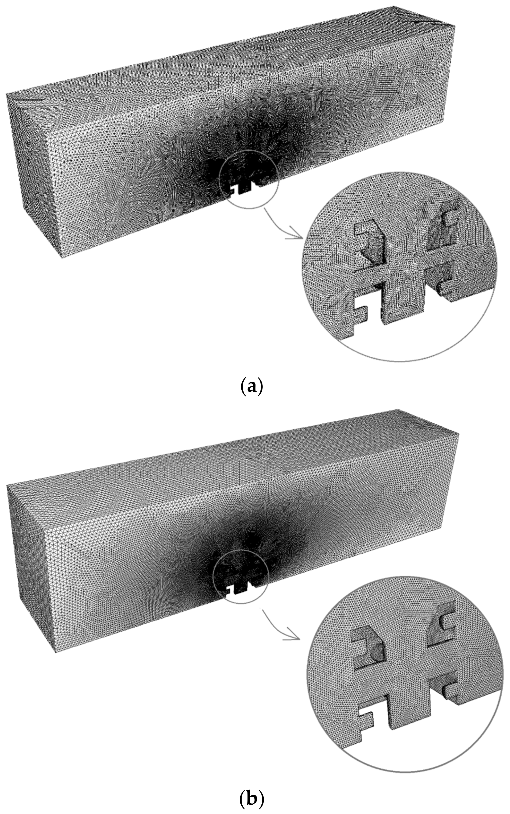
  • Determining the hydrodynamics around the AR through a CFD model. Two different configurations of the AR are analyzed in order to see which favors the most circulation for the specific area based on the value of the velocity inside the AR module.
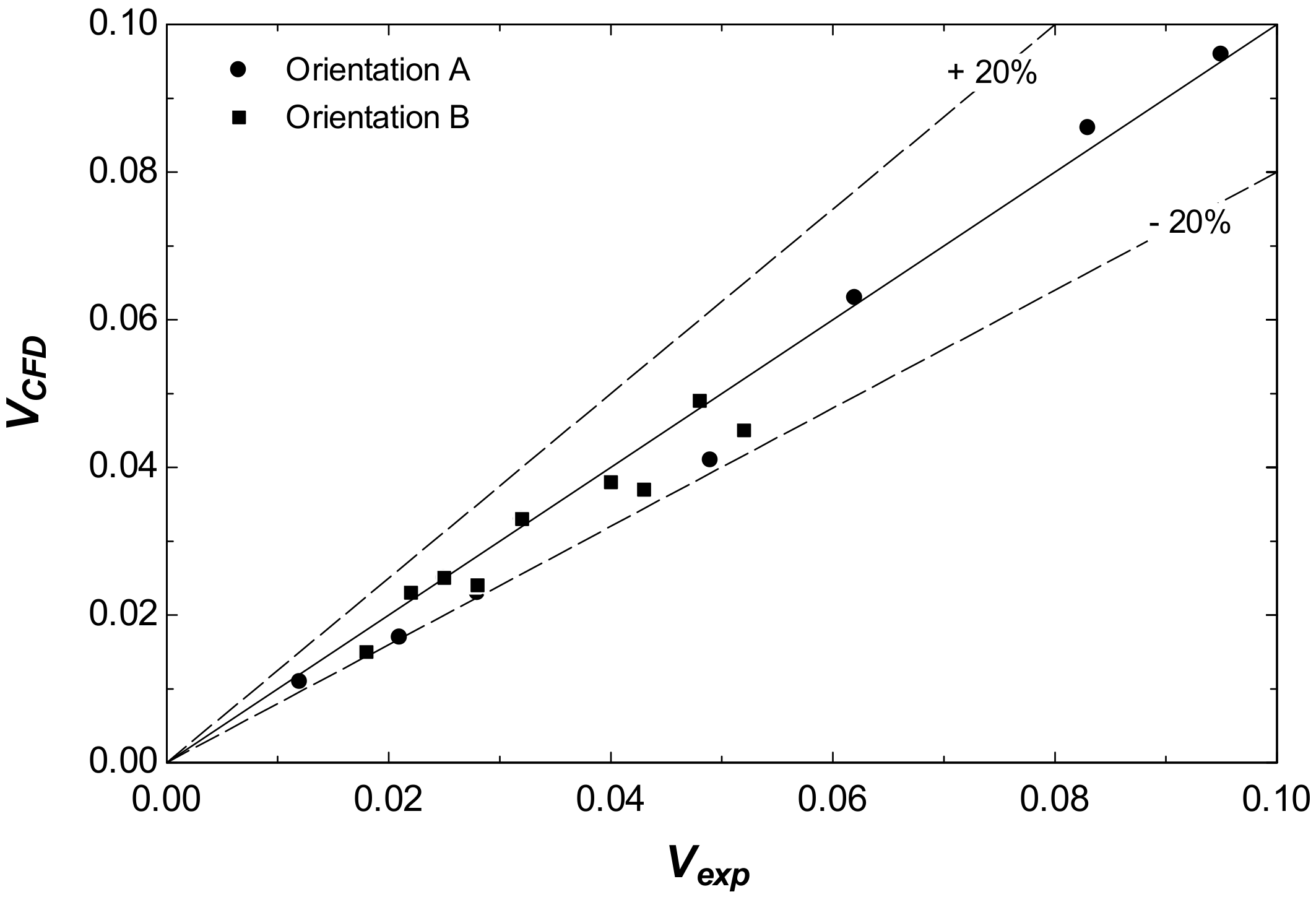
  • Validating the CFD results through towing tank tests.
To address the aforementioned objectives, the proposed methodology is applied to a case study, the Ría de Ares-Betanzos, an estuarine area located in NW Spain which has shown to be of great interest for AR operation (Figure 2).
The Ría de Ares-Betanzos is located between the Ría de A Coruña (to the W) and Ría de Ferrol (to the NE), covering a total area of about 72 km2, and with a length of 19 km, which is divided in its upper part in two branches: (i) Ares, i.e., the estuary of river Eume, and (ii) Betanzos, i.e., the estuary of river Mandeo, which are the two main tributaries to this Ría. In particular, to address the proposed objectives, three large areas characterized at specific representative locations (L1, L2, and L3) which have been previously established as of interest for AR operation [37] (Figure 2) are analyzed.

2. Materials and Methods

The methodology of the present work is illustrated in Figure 3. A hydrodynamic circulation model (HCM) (Section 3.1) was developed to characterize the circulation of the Ares-Betanzos estuary. This model establishes the current velocity against the depth in different locations. The design of cubic AR units was developed elsewhere [6,38]. The reader should bear in mind that the terms AR, AR unit, and AR module refer to the same design presented in Refs. [6,38] (Figure 4). Consequently, they are used interchangeably throughout the text. This design has two possible orientations and both were analyzed through a CFD model using the current velocity profile provided by the HCM model. The CFD model constitutes a single-phase hydrodynamic model for food delivery prediction (HMFDP) since the velocity field is characterized. Those regions with low velocities are not appropriate because the nutrient circulation is poor. The results of the CFD model were validated through towing tank tests.

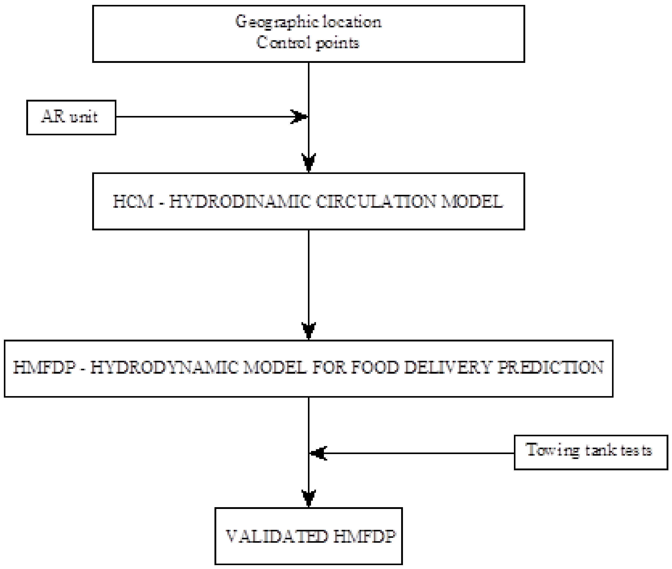
2.1. Hydrodynamic Circulation Model (HCM)

Estuaries present site-specific circulation characteristics, primarily resulting from the action of the tide and river discharges, which largely affect the operation of ARs. Moreover, during specific events, winds may play an important role driving upwelling and downwelling episodes. These characteristics should be accurately considered when designing ARs to be adapted to the hydrodynamics of the coastal area where they are intended to be deployed.
Overall, the tide is the major force driving the circulation in the Ría de Ares-Betanzos, as in the case of the rest of the Galician rías [39,40]. However, river inputs to this estuary present a larger relative importance at the time of driving its hydrodynamics compared to the Rías Baixas [41], which usually lead to a positive circulation independently of the prevailing winds. The action of winds and, in particular, the action of winds of significant speed (e.g., 10 ms−1) is relevant during upwelling and downwelling episodes [42], but not for analyzing average conditions.
On this basis, in the present study, the 3D hydrodynamic characteristics in the Ría de Ares-Betanzos under average conditions are computed, for which a representative complete spring-neap tidal cycle under average annual river inflows and average annual oceanic thermohaline water characteristics is analyzed. The results obtained are used to characterize three large areas, Figure 2, previously established as of interest for AR operation [37], where their 2D characteristics were assessed at specific locations of interest: L1, L2, and L3, with mean water depths of 21.4 m, 16.3 m, and 10.1 m, respectively [16]. The results obtained are subsequently used for AR optimization in the next sections.
To this end, in the present work, the DELFT3D FLOW [43] is applied to this coastal area. It consists in a state-of-the-art hydrodynamic model, which approximates the Navier Stokes equations under the Shallow Water and Boussinesq assumptions, which are coupled to the transport equation, allowing the computation of barotropic and baroclinic flows, resulting from river discharges and their interaction with oceanic waters. In the vertical dimension, a σ-layer grid composed of 12 layers is defined with the following resolution (%) (from upper to bottom layers): 2, 3, 5, 10, 15, 15, 15, 15, 10, 5, 3, 2. This discretization provided a good representation of the vertical structure circulation in other Galician estuaries [42], and in addition, in the present application leads to an accurate computation of the bottom flows to which AR units would be subject. With respect to the spatial discretization, 100 m of grid spacing within the Ría is considered, along with a high-resolution bathymetry dataset, which are interpolated to the numerical grid. This grid size is chosen given that similar values were used previously in other Galician rías with similar hydro-morphodynamic characteristics, providing accurate results.
The temporal discretization resorts to an alternating-direction implicit (ADI) scheme. This scheme divides the time steps in two levels, at which all equation terms are evaluated. Regarding the horizontal discretization, an Arakawa C-grid is implemented, which consists in a staggered grid with water levels being computed at the centers of the grid cells, and velocities at the midpoints of grid faces. Finally, the horizontal advection terms are computed through the Cyclic method [43].

2.2. Hydrodynamic Model for Food Delivery Prediction (HMFDP)

The AR modules are cubic shapes 1.5 m edge due to logistic restrictions [7,44]. This size allows an easy transportation by common trucks. The design is shown in Figure 4. As can be seen in this figure, an interior vertical hole of 0.6 m diameter is communicated with two horizontal holes of 0.25 and 0.45 m diameter. The objective of the vertical hole is to receive light, while the horizontal holes aim to mainly receive nutrients. Besides, nest cavities with diameters of 0.15 and 0.2 m are placed in order to allocate organisms. These dimensions were established according to the biological analysis developed in [44]. Figure 4 shows the 3D view as well as the AA and BB sections. Regarding the orientation against the current velocity, two options are analyzed in the present work.
-
Orientation A: 0.25 m diameter hole parallel to the current velocity.
-
Orientation B: 0.45 m diameter hole parallel to the current velocity.
The proposed design has been analyzed through CFD. The software OpenFOAM was employed for such a purpose. The Reynolds Averaged Navier–Stokes (RANS) conservation equations of mass and momentum have been solved. As the turbulence model, the standard k-ε has been employed. The SIMPLE algorithm was chosen for pressure–velocity coupling, and a second order upwind scheme was employed to discretize the governing equations. The computational meshes are shown in Figure 5. It can be seen that only half of the AR was analyzed by virtue of symmetry. A mesh sensibility analysis developed elsewhere [44], indicating that these meshes are appropriate. The current velocity was established as an inlet boundary condition. An outlet boundary condition was imposed at the opposite side. The reef and seafloor were modeled as no slip surfaces.

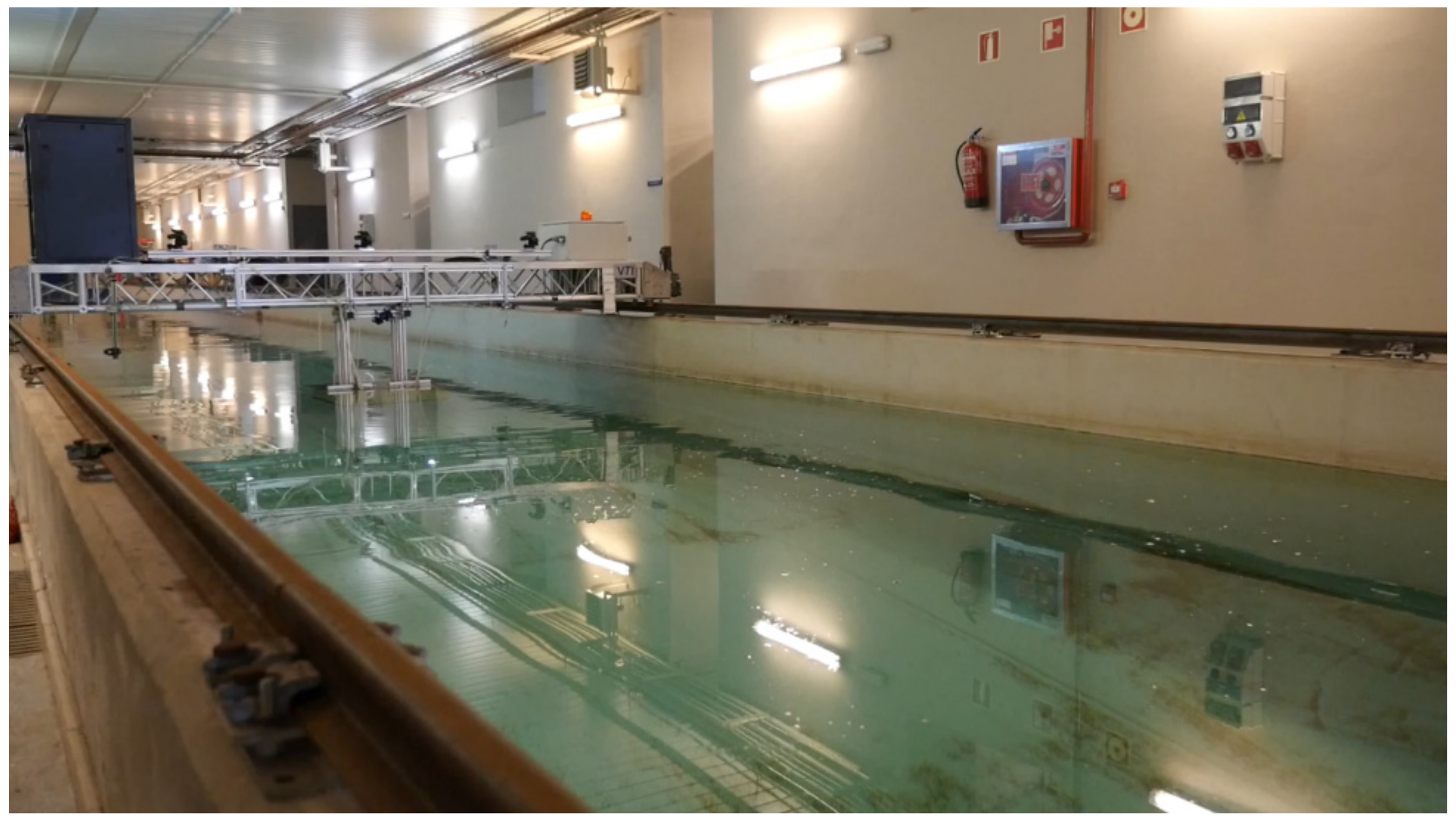
2.3. Towing Tank Tests

As mentioned above, experimental tests were carried out in order to validate the proposed HMFDP model. The tests were performed at the towing tank of Universidade da Coruña. In this facility, as there is no current generator, the model was towed by the carriage at the corresponding velocities along the entire tank, as illustrated in Figure 6. The experiments were repeated for each orientation (A and B), and the velocities that have been analyzed in the HMFDP model (shown in Table 1).
The 1:2 scale model of the AR was made in high-density polyurethane foam and reinforced with fibreglass, as can be seen in Figure 7.
The current velocity inside the vertical hole of the AR was measured using a Nortek’s Vectrino velocimeter during the test, i.e., during the towing from the beginning until the end of the tank. The output is a time series containing the values of the velocity. Then, the average of each time series was calculated to obtain the mean value of the speed for each experiment.
In order to validate the profile of the speed against depth obtained with the hydrodynamic model, the measurements were taken at two different heights: S1 (corresponding to 0.25 m from the base of the AR) and S2 (corresponding to 0.50 m from the base of the AR), as shown in Figure 7.

3. Results

This section describes the results of the hydrodynamic circulation model as well as the hydrodynamic model for food delivery prediction, and the towing tank tests.

3.1. Hydrodynamic Circulation Model results

The model is validated against ADCP data deployed in the Ría at 43°24.30′ N, 8°16.49′ W from 15 October 2007 to 19 November 2007. Figure 8 shows the velocity magnitude measured by the ADCP (dots) and obtained from the model (line) at a representative location of the water column (intermediate depth). It can be observed that the model accurately reproduces the observations, with exception of specific velocity peaks. The statistical parameters obtained are: R = 0.86, RMSE = 0.029 ms−1.
The results at each location of interest for the complete average spring-neap tidal cycle are provided in terms of site-specific velocity parameters [6] at each vertical layer (mid-water depth): (i) the mean magnitude of the currents during the tidal cycle, Vm, (ii) the mean magnitude of the current velocity during the tidal cycle with current velocities greater than V50% (velocity magnitude exceeded during half of the time), Vm50%, and (iii) the peak magnitude of the velocity throughout the tidal cycle, Vp, Figure 9.
The vertical profiles of the different parameters of interest show that the 3D hydrodynamic behavior significantly differs amongst locations. In the upper layers, the location with the figures of the velocity parameters is L2, closely followed by L3, and finally L1 with significant lower figures. L2 presents larger values than L3 throughout the water column, with significant differences at intermediate layers; however, L1 provides the largest figures at the bottom layers—slightly greater than at L2—, resulting from their more homogeneous vertical behavior. This vertical structure can be described as follows. At L1, the vertical distribution of the current velocities is virtually constant for the different velocity parameters, with somewhat lower velocities close to the surface and bottom. Instead, at L2 and L3, larger current magnitudes in upper layers are observed, reducing their magnitude with depth, progressively in the case of L2, and sharply in the case of L3 in the upper 3–4 m, below which they remain stable down to close the bottom layers.
Considering the dimensions of the AR proposed, and the size of the different numerical layers, the best representation of the current magnitude for AR design is obtained by computing the average current velocity at the three lower bottom layers (10, 11, and 12) weighted according to their size (% of the water column). Finally, the velocity parameters providing more valuable information for the design of the AR are the average parameters, both Vm and Vm50%, and not the peak velocities, Vp, attained at specific moments, which in turn are of high interest for the design of the AR in terms of stability (to determine the total weight and its distribution to avoid overturning or slide of the AR group). On these bases, the velocity parameters considered for AR modeling optimization (weighted average values at layers 10, 11, and 12) are presented in Table 1.

3.2. Hydrodynamic Model for Food Delivery Prediction Results

Due to the limitations of the facility and to minimize scale effects, the scale of the AR model used in the experiments is 1:2, i.e., half the original size. Thus, for the sake of simplicity, the results will be presented in model scale instead of real scale. In order to maintain the Reynolds number, the current velocities analyzed are twice as those shown in Table 1. According to this, the scaled current velocities and the corresponding current velocities are shown in Table 2. It is worth noting that the value 0.051 shown in Table 1 was not modeled because it is too similar to 0.055.
The velocity field in the middle of the AR module is shown in Figure 10 and Figure 11 for orientations A and B, respectively. The middle line is illustrated in red color in these figures. Both 0.074 and 0.110 ms−1 current velocities are illustrated in these figures. The other current velocities analyzed provided similar graphs to those shown in these figures and thus are not shown again.
Table 3 shows the results of the CFD analysis corresponding to each location and orientation of the AR module. As it was mentioned, the velocities were measured at two different heights.

3.3. Towing Tank Tests

Table 4 presents the results of the experiments corresponding to each location and orientation of the AR module.

3.4. Discussion

Figure 12 plots the velocities estimated by CFD against the velocities measured during the experiments in the towing tank. The results for orientation A are represented by black dots and for orientation B by black squares.
As it can be observed, the correspondence between experimental and numerical results is quite satisfactory. The difference remains under 20%. It seems that for orientation A, the difference in the results is smaller, however, no general trend can be highlighted. These results, for tests that have been carried out on such a big scale (almost real scale) and for values of the current that low, can be considered acceptable.
If velocities are analyzed considering the orientation of the AR module, some facts can be pointed out. For orientation A, the velocities inside the unit are larger than the velocities for orientation B at the same heights. What is more, in orientation A, there is an increment in velocities from point S1 to S2. On the contrary, in orientation B, the velocities remain approximately constant with height. Thus, it seems that the 0.25 m diameter hole parallel to the current velocity (orientation A) favors a higher circulation of water inside and, in consequence, the transport of nutrients.
Regarding the three different locations (L1, L2, and L3), it can be seen that there is a correlation between the current speed and the velocities inside the artificial reef. The largest values inside are obtained with the largest current speeds. Therefore, L1 is the location that will provide the higher circulation for the configuration of the proposed AR unit, followed by L2 and L3. In the three locations, the proposal is to position the artificial reef with orientation A perpendicular to the incident current in order to maximize the hydrodynamic characteristics of the design.

4. Conclusions

In this paper, the application of hydrodynamics to predict the water circulation inside an artificial reef has been presented. First, a hydrodynamic model was used to determine the characteristics of the current velocity in the studied area (Ares-Betanzos estuary). Three points of interest in the area were selected. Once these velocities were known, another hydrodynamic model was applied to obtain the water velocity profile inside the AR in order to predict food delivery, i.e., the nutrient circulation around and inside an AR. The studied AR module presents two possible orientations to the incident current. Both orientations were analyzed to evaluate their performance. Finally, the HMFDP was validated with experimental tests.
From the obtained results, it can be concluded that there is a satisfactory concordance and thus the hydrodynamic model can be used to predict food delivery. Furthermore, orientation A (0.25 m diameter hole parallel to the current velocity) of the AR unit results in the best hydrodynamic configuration of the design to improve the circulation of water and nutrients.
It is also necessary to highlight some of the main contributions of this work to the field. On the one hand, an important novelty consists of coupling a hydrodynamic circulation model for a specific coastal area with a CFD model. Although this work was applied to the Ares-Betanzos estuary, it can be extrapolated to other zones worldwide.
On the other hand, the experimental part of these studies is usually conducted in wind tunnels. However, the authors decided to perform them in a towing tank for the first time in order to analyze the suitability of this type of facility for future work. It was concluded that it is a feasible alternative, although some difficulties exist. The main ones are (1) the compromise between the scale of the model in relation to the values to be measured; and (2) the added challenges of working underwater.

Author Contributions

Conceptualization, L.S.C., M.I.L.G., R.C.; I.L., J.J.C.B. and L.C.; methodology, L.S.C., M.I.L.G., R.C.; I.L., J.J.C.B. and L.C.; formal analysis, L.S.C., M.I.L.G., R.C.; I.L., J.J.C.B. and L.C.; investigation, L.S.C., M.I.L.G., R.C.; I.L., J.J.C.B. and L.C.; resources, L.S.C., M.I.L.G., R.C., I.L., J.J.C.B. and L.C.; writing—original draft preparation, L.S.C., M.I.L.G., R.C., I.L., J.J.C.B. and L.C.; writing—review and editing, J.J.C.B. All authors have read and agreed to the published version of the manuscript.

Funding

This research was funded by Xunta de Galicia, grant number CN-10MMA003CT. This study was also funded through the collaboration agreement between Xunta de Galicia (Convenio de colaboración entre a Xunta de Galicia, a Universidade da Coruña e a Fundación da Universidade da Coruña para dar continuidade ao Proxecto de investigación de arrecife artificial—PROARR), Universidade da Coruña and the Universidade da Coruña Foundation (FUAC) to give continuity to the previous project.

Institutional Review Board Statement

Not applicable.

Informed Consent Statement

Not applicable.

Data Availability Statement

Not applicable.

Acknowledgments

The authors gratefully acknowledge the financial support from the regional government of Galicia, Xunta de Galicia, through the project CN-10MMA003CT. This study was also funded through the collaboration agreement between Xunta de Galicia, Universidade da Coruña, and the Universidade da Coruña Foundation (FUAC) to give continuity to the previous project.

Conflicts of Interest

The authors declare no conflict of interest.

Nomenclature

ADCPAcoustic doppler current profiler
ADIAlternating-direction implicit
ARArtificial reef
CARConventional artificial reef
CFDComputational fluid dynamics
GARGreen artificial reef
HCMHydrodynamic circulation model
HMFDPHydrodynamic model for food delivery prediction
NENorth East
OG-GAROne generation–green artificial reef
PIVParticle image velocity
WWest

References

  1. Rashid Sumaila, U.; Bellmann, C.; Tipping, A. Fishing for the Future: An Overview of Challenges and Opportunities. Mar. Policy 2016, 69, 173–180. [Google Scholar] [CrossRef]
  2. Visbeck, M.; Kronfeld-Goharani, U.; Neuman, B.; Rickels, W.; Shmidt, J.; Van Doorn, E.; Matz-Lück, N.; Ott, K.; Quas, M.F. Securing Blue Wealth: The Need for a Special Sustainable Development Goal for the Ocean and Coasts. Mar. Policy 2014, 48, 184–191. [Google Scholar] [CrossRef] [Green Version]
  3. Rickels, W.; Dovern, J.; Quaas, M. Beyond Fisheries: Common-Pool Resource Problems in Oceanic Resources and Services. Glob. Environ. Chang. 2016, 40, 37–49. [Google Scholar] [CrossRef]
  4. Bacher, C.; Grant, J.; Hawkins, A.J.S.; Fang, J.; Zhu, M.; Besnard, M. Modelling the Effect of Food Depletion on Scallop Growth in Sungo Bay (China). Aquat. Living Resour. 2003, 16, 10–24. [Google Scholar] [CrossRef]
  5. Carral, L.; Rodriguez-Guerreiro, M.; Tarrio-Saavedra, J.; Alvarez-Feal, J.C.; Fraguela Formoso, J. Social Interest in Developing a Green Modular Artificial Reef Structure in Concrete for the Ecosystems of the Galician Rías. J. Clean. Prod. 2018, 172, 1881–1898. [Google Scholar] [CrossRef]
  6. Carral, L.; Lamas-Galdo, M.I.; Rodríguez-Guerreiro, M.J.; Vargas, A.; Álvarez-Feal, C.; Carballo, R. Configuration Methodology for a Green Variety Reef System (AR Group) Based on Hydrodynamic Criteria—Application to the Ría de Ares-Betanzos. Estuar. Coast. Shelf Sci. 2021, 252, 107301. [Google Scholar] [CrossRef]
  7. Carral, L.; Cartelle Barros, J.J.; Carro Fidalgo, H.; Camba Fabal, C.; Munín Doce, A. Greenhouse Gas Emissions and Energy Consumption of Coastal Ecosystem Enhancement Programme through Sustainable Artificial Reefs in Galicia. Int. J. Environ. Res. Public Health 2021, 18, 1909. [Google Scholar] [CrossRef]
  8. Caballero Miguez, G.; Garza Gil, M.D.; Varela Lafuente, M.M. Institutions and Management of Fishing Resources: The Governance of the Galician Model. Ocean Coast. Manag. 2008, 51, 625–631. [Google Scholar] [CrossRef]
  9. Nogueira, C. Galicia En La Unión Europea. Una Economía Emergente. Rev. Galega Econ. 2008, 17, 1–14. [Google Scholar]
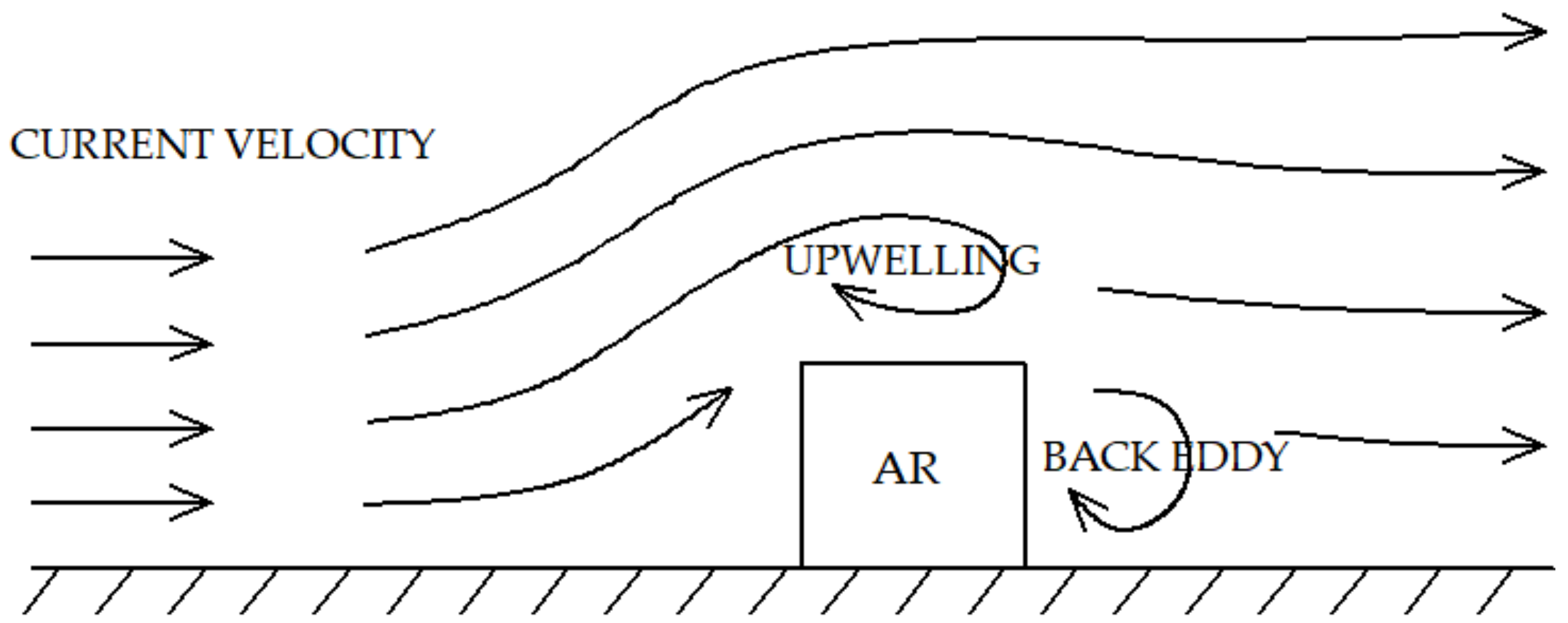
  10. Kim, D.; Woo, J.; Na, W. Intensively Stacked Placement Models of Artificial Reef Sets Characterized by Wake and Upwelling Regions. Mar. Technol. Soc. J. 2017, 51, 60–70. [Google Scholar] [CrossRef]
  11. Klaoudatos, D.; Anastasopoulou, A.; Papaconstantinou, C.; Conides, A. The Greek Experience of Artificial Reef Construction and Management. J. Environ. Prot. Ecol. 2012, 13, 1647–1655. [Google Scholar]
  12. Techera, E.J.; Chandler, J. Offshore Installations, Decommissioning and Artificial Reefs: Do Current Legal Frameworks Best Serve the Marine Environment? Mar. Policy 2015, 59, 53–60. [Google Scholar] [CrossRef]
  13. Yun, D.-H.; Kim, Y.-T. Experimental Study on Settlement and Scour Characteristics of Artificial Reef with Different Reinforcement Type and Soil Type. Geotext. Geomembr. 2018, 46, 448–454. [Google Scholar] [CrossRef]
  14. Kim, D.; Jung, S.; Kim, J.; Na, W.-B. Efficiency and Unit Propagation Indices to Characterize Wake Volumes of Marine Forest Artificial Reefs Established by Flatly Distributed Placement Models. Ocean Eng. 2019, 175, 138–148. [Google Scholar] [CrossRef]
  15. Camba, C.; Mier, J.L.; Carral, L.; Lamas, M.I.; Álvarez, J.D.; Díaz-Díaz, A.M.; Tarrío-Saavedra, J. Erosive Degradation Study of Concrete Augmented by Mussel Shells for Marine Construction. J. Clean. Prod. 2021, 9, 1087. [Google Scholar] [CrossRef]
  16. Carral, L.; Camba Fabal, C.; Lamas Galdo, M.I.; Rodríguez-Guerreiro, M.J.; Cartelle Barros, J.J. Assessment of the Materials Employed in Green Artificial Reefs for the Galician Estuaries in Terms of Circular Economy. Int. J. Environ. Res. Public Health 2020, 17, 8850. [Google Scholar] [CrossRef] [PubMed]
  17. Mo, K.H.; Alengaram, U.J.; Jumaat, M.Z.; Yap, S.P.; Lee, S.C. Green Concrete Partially Comprised of Farming Waste Residues: A Review. J. Clean. Prod. 2016, 117, 122–138. [Google Scholar] [CrossRef]
  18. Carral, L.; Lamas, M.I.; Mier, J.L.; Cartelle Barros, J.J.; Naya, S.; Tarrio-Saavedra, J. Application of Residuals from Purification of Bivalve Molluscs in Galicia to Facilitate Marine Ecosystem Resiliency through Artificial Reefs with Shells—One Generation. Sci. Total Environ. 2023, 856, 159095. [Google Scholar] [CrossRef]
  19. Wang, G.; Wan, R.; Wang, X.; Zhao, F.; Lan, X.; Cheng, H.; Tang, W.; Guan, Q. Study on the Influence of Cut-Opening Ratio, Cut-Opening Shape, and Cut-Opening Number on the Flow Field of a Cubic Artificial Reef. Ocean Eng. 2018, 162, 341–352. [Google Scholar] [CrossRef]
  20. He, D.R.; Shi, Y.M. Attractive Effect of Fish Reef Model on Black Porgy (Sparus Macrocephalus). J. Xiamen Univ. (Nat. Sci) 1995, 34, 653–658. [Google Scholar]
  21. Baine, M. Artificial Reefs: A Review of Their Design, Application, Management and Performance. Ocean Coast. Manag. 2001, 44, 241–259. [Google Scholar] [CrossRef]
  22. Haro, A.; Castro-Santos, T.; Noreika, J.; Odeh, M. Swimming Performance of Upstream Migrant Fishes in Open-Channel Flow: A New Approach to Predicting Passage through Velocity Barriers. Can. J. Fish. Aquat. Sci. 2004, 61, 1590–1601. [Google Scholar] [CrossRef]
  23. Lan, C.H.; Chen, C.C.; Hsui, C.Y. An Approach to Design Spatial Configuration of Artificial Reef Ecosystem. Ecol. Eng. 2004, 22, 217–226. [Google Scholar] [CrossRef]
  24. Bohnsack, J.A.; Sutherland, D.L. Artificial Reef Research: A Review with Recommendations for Future Priorities. Bull. Mar. Sci. 1985, 37, 11–39. [Google Scholar]
  25. Collins, K.J.; Jensen, A.C.; Lockwood, A.P.M. Fishery Enhancement Reef Building Exercise. J. Chem. Ecol. 1990, 4, 179–187. [Google Scholar] [CrossRef]
  26. Godoy, E.; Almeida, T.; Zalmon, I. Fish Assemblages and Environmental Variables on an Artificial Reef North of Rio de Janeiro, Brazil. ICES J. Mar. Sci. 2002, 59, S138–S143. [Google Scholar] [CrossRef] [Green Version]
  27. Pickering, H.; Withmarsh, D.; Jensen, A. Artificial Reefs as a Tool to Aid Rehabilitation of Coastal Ecosystems: Investigating the Potential. Mar. Pollut. Bull. 1999, 37, 505–514. [Google Scholar] [CrossRef]
  28. Tang, Y.L.; Wang, L.; Liang, Z.L.; Jiang, Z.Y.; Shi, H.W. Test of the Hydrodynamic Performance of Square Artificial Reefs. Period. Ocean Univ. China 2007, 37, 713–716. [Google Scholar]
  29. Liu, Y.; Guan, C.T.; Zhao, Y.P.; Cui, Y.; Dong, G.H. Numerical Simulation and PIV Study of Unsteady Flow around Hollow Cube Artificial Reef with Free Water Surface. Eng. Appl. Comput. Fluid Mech. 2012, 6, 527–540. [Google Scholar] [CrossRef]
  30. Liu, T.L.; Su, D.T. Numerical Analysis of the Influence of Reef Arrangements on Artificial Reef Flow Fields. Ocean Eng. 2013, 75, 81–89. [Google Scholar] [CrossRef]
  31. Fu, D.W.; Luan, S.G.; Zhang, R.J.; Chen, Y. Two-Way Analysis of Variance of Effects of Cut-Opening Ratio and Surface Shape Facing Flowing in Artificial Fish Reefs on the Flowing Field. J. Dalian Ocean Univ. 2012, 27, 274–278. [Google Scholar]
  32. Nie, Z.; Zhu, L.; Xie, W.; Zhang, J.; Wang, J.; Jiang, Z.; Liang, Z. Research on the Influence of Cut-Opening Factors on Flow Field Effect of Artificial Reef. Ocean Eng. 2022, 249, 110890. [Google Scholar] [CrossRef]
  33. Woo, J.; Kim, D.; Yoon, H.S.; Na, W.B. Characterizing Korean General Artificial Reefs by Drag Coefficients. Ocean Eng. 2014, 82, 105–114. [Google Scholar] [CrossRef]
  34. Kim, D.; Woo, J.; Yoon, H.-S.; Na, W.-B. Wake Lengths and Structural Responses of Korean General Artificial Reefs. Ocean Eng. 2014, 92, 83–91. [Google Scholar] [CrossRef]
  35. Sherman, R.L.; Gilliam, D.S.; Spieler, R.E. Artificial Reef Design: Void Space, Complexity, and Attractants. ICES J. Mar. Sci. 2002, 59, 196–200. [Google Scholar] [CrossRef]
  36. Wang, X.; Liu, X.; Tang, Y.; Zhao, F.; Luo, Y. Numerical Analysis of the Flow Effect of the Menger-Type Artificial Reefs with Different Void Space Complexity Indices. Symmetry 2021, 13, 1040. [Google Scholar] [CrossRef]
  37. Carral, L.; Alvarez-Feal, C.; Rodríguez-Guerreiro, M.J.; Vargas, A.; Arean, N.; Carballo, R. Methodology for Positioning a Group of Green Artificial Reef Based on a Database Management System, Applied in the Estuary of Ares-Betanzos (Nw Iberian Peninsula). J. Clean. Prod. 2019, 233, 1047–1060. [Google Scholar] [CrossRef]
  38. Carral, L.; Lamas, M.I.; Cartelle Barros, J.J.; López, I.; Carballo, R. Proposed Conceptual Framework to Design Artificial Reefs Based on Particular Ecosystem Ecology Traits. Biology 2022, 11, 680. [Google Scholar] [CrossRef]
  39. Gómez-Gesteira, M.; de Castro, M.; Prego, R.; Martins, F. Influence of the Barrie de La Maza Dock on the Circulation Patterns of the Ría of A Coruña (NW-Spain). Sci. Mar. 2002, 66, 337–346. [Google Scholar] [CrossRef] [Green Version]
  40. Carballo, R.; Iglesias, G.; Castro, A. Residual Circulation in the Ría de Muros (NW Spain): A 3D Numerical Model Study. J. Mar. Syst. 2009, 75, 116–130. [Google Scholar] [CrossRef]
  41. Duarte, P.; Álvarez-Salgado, X.A.; Fernández-Reiriz, M.J.; Piedracoba, S.; Labarta, U. A Modeling Study on the Hydrodynamics of a Coastal Embayment Occupied by Mussel Farms (Ria de Ares-Betanzos, NW Iberian Peninsula). Estuar. Coast. Shelf Sci. 2014, 147, 42–55. [Google Scholar] [CrossRef] [Green Version]
  42. Iglesias, G.; Carballo, R. Effects of High Winds on the Circulation of the Using a Mixed Open Boundary Condition: The Ría de Muros, Spain. Environ. Model. Softw. 2010, 25, 455–466. [Google Scholar] [CrossRef]
  43. Deltares. Delft3D-FLOW. User Manual; Delft: Deltares, The Netherlands, 2010; Available online: https://content.oss.deltares.nl/delft3d/manuals/Delft3D-FLOW_User_Manual.pdf (accessed on 3 October 2022).
  44. Lamas Galdo, M.I.; Guerreiro, M.J.R.; Lamas Vigo, J.; Ameneiros Rodriguez, I.; Veira Lorenzo, R.; Carral Couce, J.C.; Carral Couce, L. Definition of an Artificial Reef Unit through Hydrodynamic and Structural (CFD and FEM) Models. Application to the Ares-Betanzos Estuary. J. Mar. Sci. Eng. 2022, 10, 230. [Google Scholar] [CrossRef]
Figure 1. Usual velocity field around an AR.
Jmse 10 01827 g001
Figure 2. Overview of the Ría de Ares-Betanzos and its bathymetric configuration (color code), indicating the locations (L1, L2 and L3) selected as representative of the three large areas identified as of interest for AR operation (polygons), along with the main river inflows.
Jmse 10 01827 g002
Figure 3. Flowchart with the methodology employed.
Jmse 10 01827 g003
Figure 4. Design of the proposed AR. (a) 3D; (b) AA section; (c) BB section.
Jmse 10 01827 g004
Figure 5. Computational mesh; (a) orientation A; (b) orientation B.
Jmse 10 01827 g005
Figure 6. Experimental tests at the towing tank of Universidade da Coruña.
Jmse 10 01827 g006
Figure 7. (a) AR scale model; (b) location of the sensors for orientation A; (c) location of the sensors for orientation B.
Jmse 10 01827 g007
Figure 8. Comparison between the magnitude of the flow velocity registered by the ADCP (dots) and computed by the numerical model (continuous line).
Jmse 10 01827 g008
Figure 9. Vertical distribution of the velocity parameters (Vm, Vm50%, and Vp) at the selected representative locations (L1, L2, and L3).
Jmse 10 01827 g009
Figure 10. Velocity field in the middle of the AR. Orientation A. (a) 0.074 ms−1 current velocity; (b) 0.110 ms−1 current velocity.
Jmse 10 01827 g010
Figure 11. Velocity field in the middle of the AR. Orientation B. (a) 0.074 ms−1 current velocity; (b) 0.110 ms−1 current velocity.
Jmse 10 01827 g011
Figure 12. Comparison between experimental and numerical results.
Jmse 10 01827 g012
Table 1. Values of the representative site-specific velocity parameters for AR model optimization.
LocationVm (ms−1)Vm50% (ms−1)
L10.0710.101
L20.0510.078
L30.0370.055
Table 2. Scaled current velocities and corresponding real current velocities.
Scaled Current Velocity (ms−1)Corresponding Real Current Velocity (ms−1)
0.0740.037
0.1100.055
0.1420.071
0.1560.078
0.2020.101
Table 3. Numerical results.
Orientation AOrientation B
0.25 m Height (S1)0.50 m Height (S2)0.25 m Height (S1)0.50 m Height (S2)
L1Vm = 0.142 ms−10.0230.0860.0330.039
Vm50% = 0.202 ms−10.0330.1250.0490.045
L2Vm = 0.110 ms−10.0170.0630.0230.024
Vm50% = 0.156 ms−10.0250.0960.0370.038
L3Vm = 0.074 ms−10.0110.0410.0150.025
Vm50% = 0.110 ms−10.0170.0630.0230.024
Table 4. Experimental results.
Orientation AOrientation B
0.25 m Height (S1)0.50 m Height (S2)0.25 m Height (S1)0.50 m Height (S2)
L1Vm = 0.142 ms−10.0280.0830.0320.104
Vm50% = 0.202 ms−10.0320.1030.0480.052
L2Vm = 0.110 ms−10.0260.0620.0220.028
Vm50% = 0.156 ms−10.0250.0950.0430.040
L3Vm = 0.074 ms−10.0120.0490.0200.025
Vm50% = 0.110 ms−10.0260.0620.0220.028
Publisher’s Note: MDPI stays neutral with regard to jurisdictional claims in published maps and institutional affiliations.

