1. Background and Motivation
The population of coastal watersheds around the United States (US) has been increasing over the last several years [
1], and in 2010, as much as 3% of that population is living within the zones classified as 100-year coastal flood hazard areas [
2]. If we include the combined 100-year and 500-year flood hazard areas for both the riverine and coastal areas over the entire US, that amount increases to approximately 10% [
3,
4]. These coastal areas are vulnerable to storm damage from tropical storms and hurricanes. There is a heightened risk in coastal areas due to population growth [
5], and the state of North Carolina specifically experiences vulnerabilities to coastal storm damage due to the state’s geographic and infrastructure features [
6]. Total water level (which includes tides, waves, winds, and rainfall-runoff) modeling during tropical cyclone events, including estimates of freshwater rainfall-runoff, is critical for accurately predicting future flooding in coastal cities, specifically as it pertains to long-term risk assessment [
7]. In these coastal (riverine–estuarine) zones, there is a significant NOAA service gap regarding freshwater flows, i.e., significant freshwater flows in some coastal plains are not currently accounted for in many of the operational model forecasts [
5,
8]. Numerical prediction of flood stage in these riverine–estuarine areas represents a significant challenge due to the presence of compound flooding, herein defined to be synonymous with total water level modeling.
Multiple research initiatives are underway to provide total water level prediction for tidally influenced coastal rivers, including extending existing oceanic models upstream and riverine models downstream. In the first paradigm, the oceanic model is typically extended beyond the tidal zone, and river flows are provided by either US Geological Survey (USGS) gauge information or hydrology/hydraulic models. There are many instances of oceanic models using USGS gauge observations to provide freshwater flow boundary conditions, including (among others) NOAA’s Tampa Bay, Chesapeake Bay, and Delaware River and Bay Operational Forecast Systems [
9,
10,
11]. As efforts to extend 2D models upland proceed, so do efforts to extend both 1D and 2D upland, riverine models closer to the oceanic boundary by incorporating oceanic forcings [
12,
13,
14]. Hydraulic models of tidally influenced rivers have been implemented by the National Oceanic and Atmospheric Administration (NOAA) in at least five locations [
8]. Efforts have also been undertaken to supply existing 1D and 2D models with downstream boundary conditions, including storm surge and tidal information, such as the Hydrologic Engineering Center’s River Analysis System (HEC-RAS) [
15,
16]. As yet, no upland river model including hydrologic (river network) modeling has been operationally coupled with an oceanic model over broad regions to predict the total water level interactions known to exist in tidal estuaries.
In 2010, the ADvanced CIRCulation (ADCIRC) surge guidance modeling system (ASGS [
17]) was expanded to include riverine flows from a hydrologic model (ASGS-STORM [
5,
18]). This system extended the ADCIRC model into portions of both the Tar and Neuse River basins for the North Carolina area [
18,
19]. ASGS-STORM was run initially for Hurricane Earl and has been used since to provide guidance for many of the tropical cyclones that have affected North Carolina, e.g., Hurricane Irene [
18]. Recent studies utilized the ADCIRC model with connections to an atmospheric model (Weather Research Forecast-WRF), hydrology model (EF5), and behavior and traffic model to determine evacuations in the North Carolina area during tropical cyclones [
20,
21]. Other researchers have also worked at including upland riverine flooding with other hydrologic and hydraulic models (e.g., [
22,
23,
24,
25]). Additionally, total water level forecasts have been produced in the Chesapeake Bay region using the 3D ELCIRC model [
26].
As both 1D and higher-dimensional models become available in riverine areas, the question naturally arises, under what conditions should a modeler implement a 1D river hydraulic model instead of a 2D or 3D model? The answer to this question does not have a single answer because the relative skill and cost of both types of models will depend on the particular morphologies of the river under study [
27,
28]. Horritt and Bates [
28] compared the skill and accuracy of three models of a 60-km stretch of the Severn River in the UK. The three models included the HEC-RAS (1D) and two 2D models: LISFLOOD-FP, a raster-based inundation model that uses 1D channel flow and 2D floodplain flow, and TELEMAC-2D, a model that uses Galerkin’s method of weighted residuals to solve the 2D shallow water (Saint-Venant) equations of free surface flow over an unstructured mesh. The authors were surprised to find that for their river morphology, when given a sufficiently resolved DEM raster onto which HEC-RAS results might be projected, the 1D HEC-RAS model proved a more robust and accurate predictor of flood flowrates than both 2D models. Specifically, their methodology included calibrating the models’ channel and floodplain roughness, once using flood wave travel times and once using flood inundation gathered from satellite imagery. Further, the 1D HEC-RAS was the model that showed the greatest agreement between both calibrations’ roughness values and, thus, was deemed the most insensitive to methods and the most reliable. This is partly due to the limited calibration scope and the channel morphology. Specifically, their model domain consisted of a river with steep, well-defined channel sides, which means that, even at times when water levels rapidly rise or fall, the channel sides prevent significant lateral flows. The authors expect that, given a more spatially variable descriptor of 2D flow and/or in the case of a stream of different morphology, the 2D models might prove more accurate. Recent work by Gori [
16] looked at compound flooding extents using a 1D/2D model of HEC-RAS for the Cape Fear River basin in North Carolina. They used their model to examine the influence of storm surge and rainfall on compound flooding. Results indicated that rainfall bands that accompany the eyewall of a tropical cyclone tend to lead to flooding in the coastal area from both rainfall and storm surge, especially if the peak rainfall and peak storm tide occur simultaneously. Rainfall bands that proceed storms in inland areas can drive increases in river levels ahead of the storm and in river flows as the storm makes landfall in coastal regions.
This is highly relevant to the problem of incorporating HEC-RAS, or any 1D/2D river hydraulic model, as an intermediate model for river flood prediction in coastal areas. If 1D or 2D models were proven to always be more accurate at predicting river behavior, regardless of morphology or modeling methodology, the question of what model to use in a particular area would be as simple as determining the lowest cost method that exhibited adequate accuracy. However, their findings suggest that each river to be modeled should be examined with respect to morphology and expected flow conditions to determine which modeling approach is appropriate. Horritt and Bates [
28] showed that a 1D model is more accurate in a domain with steep sidewalls. However, in a relatively flat river, at the confluence of multiple rivers, or as a river nears its mouth, lateral flows may be more significant, and 2D models may be more accurate.
Pappenberger et al. [
27] approach the problem of describing the uncertainty of models, such as HEC-RAS, by identifying possible sources of uncertainty in numerical parameter selection (e.g., timestep and time weighting), physical parameter selection (topographic measurements and roughness estimates), and boundary conditions (input and output hydrographs). They then use an automated assessment method to describe the response surface of the model to these variables in a combined fashion. The assessment was performed for two different river stretches, which showed differing sensitivities. Their findings confirm some conventional wisdom, namely that distributed model parameter information leads to more accurate modeling of river response. However, the authors demonstrate that this uncertainty problem is inherently more tractable with a 1D model. They suggest that, since uncertainty is always present in any description of the real world, a more detailed model of a river (i.e., a 2D or 3D model) will not necessarily be more reliable than a simpler one, and that instead, modelers must take into account the reliability of their data and the origin of their parameter estimates in order to determine whether a particular model is appropriate.
Comparisons of these sorts on particular domains are relatively uncommon, perhaps due to the significant cost associated with developing such models in the first place or the paucity of data. The research presented in this paper looks to undertake a systematic comparison of several different coupling techniques: hydrologic, hydraulic river models, and hydrodynamic coastal models, as applied to the Tar River Basin in North Carolina. This basin presents a unique and valuable testbed for a direct comparison of 1D and 2D river forecast models for three reasons. First, the river basin is a tidally influenced river of economic importance to the region, including multiple municipal communities that have experienced flooding during extreme tropical cyclone events, such as Hurricanes Floyd (1999), Matthew (2016), and Florence (2018). Second, NOAA resources have been expended to develop detailed models of this region. Third, other studies have analyzed riverine systems in the coastal delta plain with a shallow bottom slope in the riverine areas (i.e., Louisiana and Texas deltas). In contrast, this study will examine a river morphology that has a far steeper bottom slope, which leads to river channels in the coastal plains that are above mean sea level.
This paper will explore several different research objectives: examine the pros/cons of different coupling methods (direct/intermediate), compute the model systems’ accuracy, and measure the computational cost of the different methods. In particular, the coupling study will look at boundary information when a hydraulic model (1D HEC-RAS) is used as a connector (so-called “middleware”) between hydrologic and hydrodynamic models and determine whether it can reduce the simulation time and improve the accuracy of the guidance in total water levels during a tropical event. Additionally, as part of the coupling study, we will examine using a coarse vs. fine grid for the hydrodynamic model to determine which provides the most accurate downstream boundary conditions for the HEC-RAS model. Lastly, we will determine if adding a hydraulic model between the hydrologic and hydrodynamic models provides an immediate possibility of including the riverine areas while also reducing the simulation time, as compared to a modeling system that directly couples the hydrologic model to the coastal hydrodynamic model. The goal of this research is to provide guidance for model users who are seeking to forecast storm floods in tidally influenced rivers. By empowering engineers, emergency planners, and other public and private entities to better predict flood response, the ultimate harms of storms in terms of economic losses and loss of life will be reduced. However, more rigorous studies using HEC-RAS as middleware between a hydrologic model and ADCIRC for total water level prediction in coastal areas are needed to vet this promising option.
Note that we have chosen to focus on the 1D (unsteady) version of the HEC-RAS for three reasons: (1) 1D HEC-RAS models have been developed and calibrated for many of the major rivers and tributaries in the US as part of FEMA’s Floodplain Mapping Program, hence that extensive investment in model development expedites the timeline to an operational system; (2) 1D HEC-RAS is much less computationally intensive than 2D models, and one of our objectives is to assess computational cost vs. accuracy; and (3) 2D HEC-RAS has as its theoretical basis the same shallow water equations as ADCIRC (although they do differ in their numerical solution algorithm), so using 2D HEC-RAS as middleware would offer no computational advantage over running ADCIRC upstream to the hydrologic model’s handoff point (which is one of the coupling strategies studied herein).
The outline of the paper is as follows:
Section 2 presents the different models used in the coupled model systems, including boundary conditions for the hydraulic model, followed by coupling techniques and analysis methods;
Section 3 discusses the results from these different coupling schemes within the Tar River basin of North Carolina for two different tropical cyclones and a tropical storm;
Section 4 discusses results; and
Section 5 provides conclusions and future work.
2. Individual Models and Coupled Model Systems
To get an accurate total water picture for tidally influenced rivers, we need to follow the water from the atmosphere to coastal discharge. Often, each stage of this hydrologic process is modeled independently with little or no regard to what the neighboring models are doing. In this section, we first present the individual models used for the upper riverine region (hydrologic), coastal region (hydrodynamic), and intermediate riverine region (hydraulic). We then present five possible ways to couple these models and provide the methodology used to evaluate the proposed coupling schemes. Since the primary focus of this work is to evaluate the interaction of these models, only brief descriptions of the individual models are provided; interested readers are encouraged to examine more background and technical details in the references. We also note that for each model category, there are a wide variety of models found in practice. Since a primary objective of this work is to evaluate HEC-RAS as middleware (including coupled strategies) between an upstream hydrologic model and downstream hydrodynamic model, the results can also be used to provide guidance for other choices when using hydrologic or hydrodynamic models.
2.1. Hydrology Model: HL-RDHM
It is first necessary to route precipitation over the relevant watershed into the main river channel. Based on previous work [
18], we used the Hydrology Laboratory—Research Distributed Hydrologic Model (HL-RDHM), which was developed by the National Weather Service Office of Hydrologic Development [
29]. HL-RDHM is an inherently physics-based, measured-parameter model. HL-RDHM utilizes the Sacramento Soil Moisture Accounting model with a heat transfer component, which combines rainfall estimates with a parameterized calculation (using a priori datasets developed from observed data) of soil moisture to determine each grid cell’s effective runoff; as such, it requires gridded parameter datasets for eleven spatially variable parameters. These runoff estimates are then fed into the routing model to generate total streamflow estimates for each grid cell.
Channel routing in HL-RDHM is achieved using kinematic wave approximations based on specified rating curves. This routing model uses HL-RDHM’s structured grid and an a priori connectivity network containing prevailing channel flow directions to determine flow quantity and depth at each grid cell and timestep. The channel routing model solves the kinematic wave equations for hillslope flow and channel flow based on the assumption that gravity and friction are the only significant forces acting on the water body; full equations can be found in Koren et al. [
30]. The channel routing model requires estimates of seven spatially variable parameters.
In this study, HL-RDHM is utilized to generate an upstream boundary condition for the hydrodynamic and hydraulic models in the different coupled modeling schemes. The inherent (parameterization) uncertainty in HL-RDHM is mitigated using a 128-member ensemble approach, which includes both a priori and calibrated datasets, as employed within the ASGS-STORM system [
18], which has been shown to have operational skill. HL-RDHM flows are used as boundary conditions for downstream models. Since we are most interested in matching historical streamflow records, we employ the Nash-Sutcliffe Model Efficiency [
31] to determine which ensemble member “best” matches the historical streamflow record for each test case.
2.2. Hydrodynamic Model: ADCIRC
At the coastal interface, it is necessary to have a hydrodynamic model capable of ingesting streamflows at river boundaries. ADCIRC, an unstructured finite element hydrodynamic model that solves the 2D depth-integrated Generalized Wave Continuity Equation for water surface elevation and the momentum equations for velocity, was chosen for this work [
32,
33,
34]. It has been in use for over 30 years to model coastal phenomena (hurricane planning [
35], waves [
36], baroclinic effects [
37], tidal [
38], and storm surge impact predicting in coastal regions [
5,
6,
39]. River boundary conditions were added for the Mississippi, Atchafalaya, and Pearl River systems [
40,
41]; however, these river systems have low slopes and are near mean sea level (MSL) and, thus, do not pose the same challenges that higher-slope rivers above MSL do. More recently, the operational surge guidance system was configured to include river discharge in the Tar and Neuse River basins in North Carolina [
5,
18]; this study builds on that work by further examining the coupling mechanism. In particular, ADCIRC was modified for this study to include a river model for the Tar and Neuse basins with channel geometries/parameters determined from observed river behavior [
19].
Two versions of the hydrodynamic model are utilized: (1) a high-resolution representation of the riverine areas referred to as “fine ADCIRC”, where the upper reaches of the riverine areas are resolved within the ADCIRC model (taken directly from a previous study [
42]); and (2) a version without any refinement in the riverine area referred to as “coarse ADCIRC”, where the rivers are not included in the mesh, although the domain extents are the same in the study area. Meteorological forcing for each event used in this study is summarized below in
Section 3.1, and the open ocean boundary was specified using equilibrium M2, S2, N2, K2, K1, O1, P1, and Q1 tidal frequencies drawn from the Eastcoast 2001 tidal database [
43]. A time step of 0.5 s was used to simulate each event.
2.3. Hydraulic Model: HEC-RAS
For the intermediate river model, we used the Hydrologic Engineering Center River Analysis System (HEC-RAS) developed by the Hydraulic Engineering Center of the Army Corps of Engineers [
44]. HEC-RAS is a popular model for the prediction of river flooding and has been used extensively throughout the United States and abroad for assessing the behavior of rivers during high-flow events [
7,
22,
45], flood inundation mapping [
46], flash flood prediction [
47], and many other applications. HEC-RAS can be run in either 1D or 2D mode, although the latter is a relatively recent addition, so 1D studies dominate the historical floodplain mapping literature. Thus, there is a rich archive of calibrated and validated 1D models to draw on for developing compound flood modeling systems. Therefore, for this and other reasons discussed in
Section 1, we have chosen to focus on 1D in this work. Any subsequent reference to HEC-RAS in the remainder of this manuscript will imply 1D unsteady HEC-RAS.
In 1D, HEC-RAS can be considered a distributed model, which takes inputs of bathymetry and roughness at multiple cross-sections in a river, and is typically calibrated to match observed system behaviors, generally using Manning’s roughness term. HEC-RAS solves the full 1D form of the Saint-Venant equations (continuity and momentum), known as the dynamic wave equations, assuming mixed sub- and supercritical flow regimes to provide the incremental change in flow rate (Q) and water surface elevation (z) at each cross-section and timestep. Additional information about the formulation of the 1D equations and how they are solved in HEC-RAS software is published by the US Army Corps of Engineers [
44].
NOAA’s Office of Hydrologic Development produced a 1D HEC-RAS model of the Tar River Basin extending from Tarboro (located near the 8m contour) well into the tidal zone of the Pamlico River near Washington, NC, calibrated to extreme storm events [
48]. We utilized this 1D HEC-RAS model of the Tar River Basin without making any adjustments to cross-sections or parameters because the goal of this research was to use developed models (“out of the box”) to investigate each model’s ability to simulate flooding in a coupled model system.
Figure 1 shows this HEC-RAS model (white centerline and gray cross-sections) with the USGS gauge locations labeled, black outlines denoting the HL-RDHM model extents in the riverine region, and ADCIRC grid size (meters) shown by colored contours; notice the finely resolved river channel (down to 50m) in the ADCIRC fine panel.
For this study, HEC-RAS was run in unsteady, mixed-flow mode, which requires time-variable boundary conditions at the upstream and downstream extents of each reach. External boundary conditions can be supplied as stage time-series, flow time-series, or both. Run times vary based on the event, but computations were performed every five seconds with boundary condition input at one-hour intervals and model output every fifteen minutes.
2.3.1. Hydraulic Model Boundary Conditions
The first step in this modeling effort is to determine appropriate boundary conditions for the HEC-RAS model. To aid in this process, Hurricane Irene was selected from the suite of evaluation events because it exhibits both significant river flows and downstream storm surges. In this study, two basic paradigms can be used to provide boundary conditions to HEC-RAS: (1) force the hydraulic model directly using the streamflows output by the hydrology model (HL-RDHM) or (2) force the fine-grid hydrodynamic model with the hydrology output and then use ADCIRC output to force the hydraulic model. Throughout this section, flows and stages labeled “ADCIRC” are derived from the second paradigm while those derived using the first are denoted by “RDHM”.
The following three methods were tested for the upstream boundary conditions: (1) flow values taken directly from HL-RDHM, (2) stage values from ADCIRC, and (3) flow values from ADCIRC. It should be noted that when comparing the RDHM-derived boundaries to the ADCIRC-derived boundaries, there is a difference in the location of the boundary. The location for the hydrology runoff information passed to HEC-RAS is different than the location used to pass information to ADCIRC. This is because the HEC-RAS model begins near the USGS gauge at Tarboro, North Carolina, which is approximately 7 miles downstream of the ADCIRC boundary (see
Figure 1: note the area above the HEC-RAS cross-sections). In these 7 miles, Fishing Creek joins the Tar River, which means that the RDHM flow boundary condition uses a 1D kinematic wave model to route waters through that confluence, whereas the ADCIRC boundary conditions use a 2D dynamic wave model to do the same.
The location of the downstream boundary condition for the HEC-RAS model is in the vicinity of the USGS gauge in the Pamlico Sound near Washington, North Carolina. The following three downstream boundary conditions were considered initially: (1) stage values from ADCIRC, (2) flow values from ADCIRC, and (3) a constant stage value of 0 ft above the mean sea level. Initial tests with the downstream flow boundary showed that flow alone was not sufficient to define the behavior of the river. This is because the flow in the Tar River is typically subcritical at this point, so without the stage specified downstream, the dynamic wave equation used in HEC-RAS has an indeterminate result for the water surface profile, which leads to stage values that continue to increase. Therefore, method two was eliminated, and further tests included only options one or three for the downstream boundary.
2.3.2. Verification of Boundary Conditions
At the time of this study, Hurricane Irene had the most complete data coverage for the Tar River during the event, so it was used for the boundary condition verification study. For each of the six boundary condition combinations (three upstream and two downstream), the resulting HEC-RAS flow and stage were compared to gauge data at USGS stations along the Tar River within the model domain. There are three internal stations available at or near Rock Springs, Greenville, and Grimesland (the locations are shown in
Figure 1). The results are similar for all three stations and are described qualitatively (complete graphical comparisons are provided in Bush [
49]).
For the Greenville station, the streamflow derived from RDHM flow-driven boundaries shows results closest to peak values and values closest to low-flow conditions during the receding limb portion of the event. ADCIRC stage-driven results overestimate flows at all periods of the storm, while ADCIRC flow-driven results underestimate peaks and overestimate falling limb flows. Meanwhile, flow comparisons for the downstream stage boundary condition indicate that this value does not significantly affect the flow results at this station. For the stage results at the Greenville station, we note that both flow-derived stage predictions underestimate the peak, while the ADCIRC-stage derived results best match the peak value. However, only the RDHM flow-driven models show excellent agreement with observed gauge heights on the receding limb.
The remaining two stations only record stage values, so no flow comparisons are available. The upper riverine station (Rock Springs) showed similar results to Greenville. However, at the lower river station (Grimesland), the results are influenced by both storm surge and riverine flows, as evidenced by two peaks in the gauge observations. At this station, it was evident that the constant stage downstream boundary was unable to capture the initial surge peak in the river; however, the ADCIRC stage tended to overestimate the surge peak. For the upstream boundary conditions, the behavior mimics that at upstream gauge stations; namely, both flow-driven predictions underestimate the peak runoff stage, while the ADCIRC stage results match the peak well, and only the RDHM flow-driven results are able to accurately capture the receding limb. However, the ADCIRC stage results produced a reasonable representation of the falling limb baseflows.
In summary, results indicate that no single upstream boundary condition best captures observed behaviors. Rather, upstream flow specifications are more suitable when one is primarily interested in accurate flow rates and/or receding limb behavior, while stage boundaries are best for accurate peak elevations. Furthermore, accurate downstream stage boundaries are required to capture the surge response in the river.
2.4. Coupling Methodologies
For the purpose of this research, couplings were implemented in a loose, one-directional fashion; each model was run independently, with results being passed as input boundary forcings for the next model. Since we are most interested in exploring the optimal way to include hydraulic “middleware” modeling, the coupled schemes are described by how HEC-RAS is implemented within them: namely, what order the models are coupled and what information is passed as boundary conditions to HEC-RAS. Each of the coupling schemes to be analyzed is discussed in the sections that follow.
2.4.1. Coupling Scheme 1—Existing ASGS-STORM Operational System
Figure 2 shows the coupling scheme of the existing ASGS-STORM system, which has been utilized since 2011 within the coastal North Carolina area [
5,
18,
42]
1. This coupling includes only the HL-RDHM and ADCIRC (fine ADCIRC) models, where the flow from HL-RDHM is passed directly to ADCIRC at the boundaries in the upland riverine areas. This coupling scheme is used to provide a baseline for comparison to the various HEC-RAS couplings.
2.4.2. Coupling Scheme 2—HEC-RAS Middleware
The basic premise of this coupling scheme is that HEC-RAS would sit between the hydrology model and the hydrodynamic model in order to provide more detailed guidance in the riverine region and allow the inclusion of hydraulic structures, such as bridges. At the upstream boundary, HEC-RAS receives flow rates from HL-RDHM, and at the downstream boundary, it receives stages from ADCIRC. In this scheme, there are two options for the downstream: (1) run fine ADCIRC with riverine forcing to estimate total stage height (tide, surge, and riverine) at the HEC-RAS boundary or (2) run coarse ADCIRC with no riverine flows to estimate stage height. The second option would provide faster computational times due to the use of a coarse ADCIRC grid (no added resolution in the riverine areas), thus making it an attractive option for widespread adoption by a real-time guidance system. A schematic of the data transfer for both options is shown in
Figure 3, where panel (a) depicts the fine ADCIRC option with riverine forcing and panel (b) depicts the coarse ADCIRC option.
2.4.3. Coupling Scheme 3—HEC-RAS Sequential
In this scheme, the models would be run sequentially, with HEC-RAS receiving all forcing directly from ADCIRC. Flow results from the HL-RDHM model are passed to the fine ADCIRC model; then, the HEC-RAS model is forced with results from fine ADCIRC at the upstream boundary (either flow or stage) and either fine or coarse stages at the downstream boundary (see
Figure 4). This coupling scheme can be compared directly to the current operational method (scheme 1) to determine the relative accuracy of ADCIRC and HEC-RAS while also isolating the errors at either boundary. Note that for the HEC-RAS upland boundary, both flow and stage forcings were analyzed for suitability, and the most accurate condition was chosen for each event, as determined based on comparisons to gauge data near the boundary. Stage forcings were determined to be most accurate for all cases examined. Additionally, if such a scheme were implemented in practice, fine ADCIRC would be used for both the upstream and downstream boundaries, but we examine coarse ADCIRC to explore the sensitivity of HEC-RAS to the downstream stage.
2.5. Evaluation Procedures
The ultimate goal of this study is to assess if HEC-RAS can be used to accurately predict riverine behavior within the tidal river zone when forced with an upstream hydrology model and downstream hydrodynamic model, ideally similar to coupling scheme 2b for an efficient operational system. As such, each coupling scheme will be evaluated to determine its individual merit (accuracy) within the riverine region and associated computational cost.
The coupling methodologies will be evaluated for three extreme events. Each event includes hindcast comparisons to gauge data at USGS stations (the locations are shown in
Figure 1). Hydrographs at these stations are plotted in a uniform style for easy comparison. The color of the HEC-RAS boxes in
Figure 3 and
Figure 4 corresponds to the color of the results for that coupled model in subsequent sections: blue/dashed-cyan for middleware with the downstream stage taken from fine/coarse ADCIRC and red/dashed-pink for sequential with the same downstream convention. When comparing models, the results taken directly from ADCIRC (existing ASGS-STORM system without any HEC-RAS coupling) will be shown in green. For many hydrographs, there will be little difference between the dashed and solid lines. Finally, observed data will be shown with solid black lines.
In addition to qualitative hydrograph comparisons, we also use error measures for the peak timing and surge. These errors are obtained by comparing the values from the different model results with those from the observations. These errors are then shown versus the distance along the stream, and the same colors mentioned above are used for each coupling scheme, with the addition of different shapes to delineate the fine ADCIRC versus coarse ADCIRC results. Finally, comparisons of inundation extents are examined for each event. These comparisons were made qualitatively due to the lack of data on the flooding extent within the riverine areas.
3. Results and Discussion
To compare the different coupling schemes and the differences between the HEC-RAS and ADCIRC models, two tropical cyclones and a heavy precipitation event were examined within the North Carolina study area. The addition of a precipitation-only event provides insight into model behavior under runoff dominant conditions. Event-specific meteorological forcing is described in
Section 3.1.
Since the primary intent of this study is the response of the riverine areas, the comparison of the results from each event will focus solely upon USGS gauge stations [
50] and inundation extents of the different modeling schemes. However, wind data from NDBC [
51] and NOS buoys [
52] were used to verify that the ADCIRC model input was appropriate.
For each event, the accuracy of the applied riverine boundary conditions is examined to provide additional guidance when interpreting actual coupled model results. To this end, observations from the two USGS gauge locations located near the upstream and downstream boundaries of the HEC-RAS model are compared to the coupled model results and applied boundary forcing, as applicable. Then, observations from the three interior gauges are compared to the coupled model results. Finally, the resulting inundation extents of the models are compared.
3.1. Events Used for Study
Hurricane Irene made landfall in North Carolina as a Category 1 hurricane. It struck near Cape Lookout, NC, on 27 August 2011 before moving north along the coast and Outer Banks. The strongest sustained winds observed from the system during landfall were experienced just southeast of Pamlico Sound and exceeded 40.2 m/s [
53]. Hurricane Irene brought high rainfall totals (exceeding 38 cm [
53]) to the area; however, it did not produce significant flooding at Tarboro. At Greenville, river stages exceeded the NOAA-designated flood stage by 61 cm, and at Washington, stages exceeded flood levels by 91 cm. This indicates that significant lateral inflows were present in the river system within the model domain, thus making it a good test case. Precipitation values were obtained from the Stage IV radar products [
54], and hindcast wind forcing was provided by Oceanweather, Inc [
55].
Hurricane Floyd provides a different analysis as it was proceeded by Hurricane Dennis, which made landfall and delivered almost 25 cm of rain in the Pamlico Sound area a month prior to Floyd. This resulted in increased soil moisture, which led to higher rainfall-runoff during Floyd. Hurricane Floyd made landfall as a Category 2 hurricane near Cape Fear, North Carolina, on 16 September 1999, and continued along the eastern part of North Carolina [
56]. The storm surge from Hurricane Floyd was approximately 1m along the coastal North Carolina region; however, the most significant impact was the extensive rainfall that fell before and during the storm with totals as high as 38 to 50 cm [
56]. Damage costs due to Floyd were around USD 6.9 billion, with a significant amount of the damage occurring due to freshwater flooding [
56]. Precipitation to drive the HL-RDHM hydrology model was obtained from TRMM satellite products [
57], and hindcast wind forcing for Hurricane Floyd was provided by ARA [
58].
The final test case is an extreme rainfall event during April of 2003. This event caused high rainfall-runoff and streamflows for the area but had weak winds; thus, the event had little to no surge in the riverine areas, allowing a comparison of coupling schemes that are purely runoff driven. Wind speeds off the coast of North Carolina were below hurricane strength for the entire month of April and were examined at several offshore buoys along the North Carolina coastline to ensure that the time frame analyzed would not have a surge component in the riverine areas. Precipitation values were obtained from the Stage IV radar products [
54], and no wind forcing was utilized during this time period.
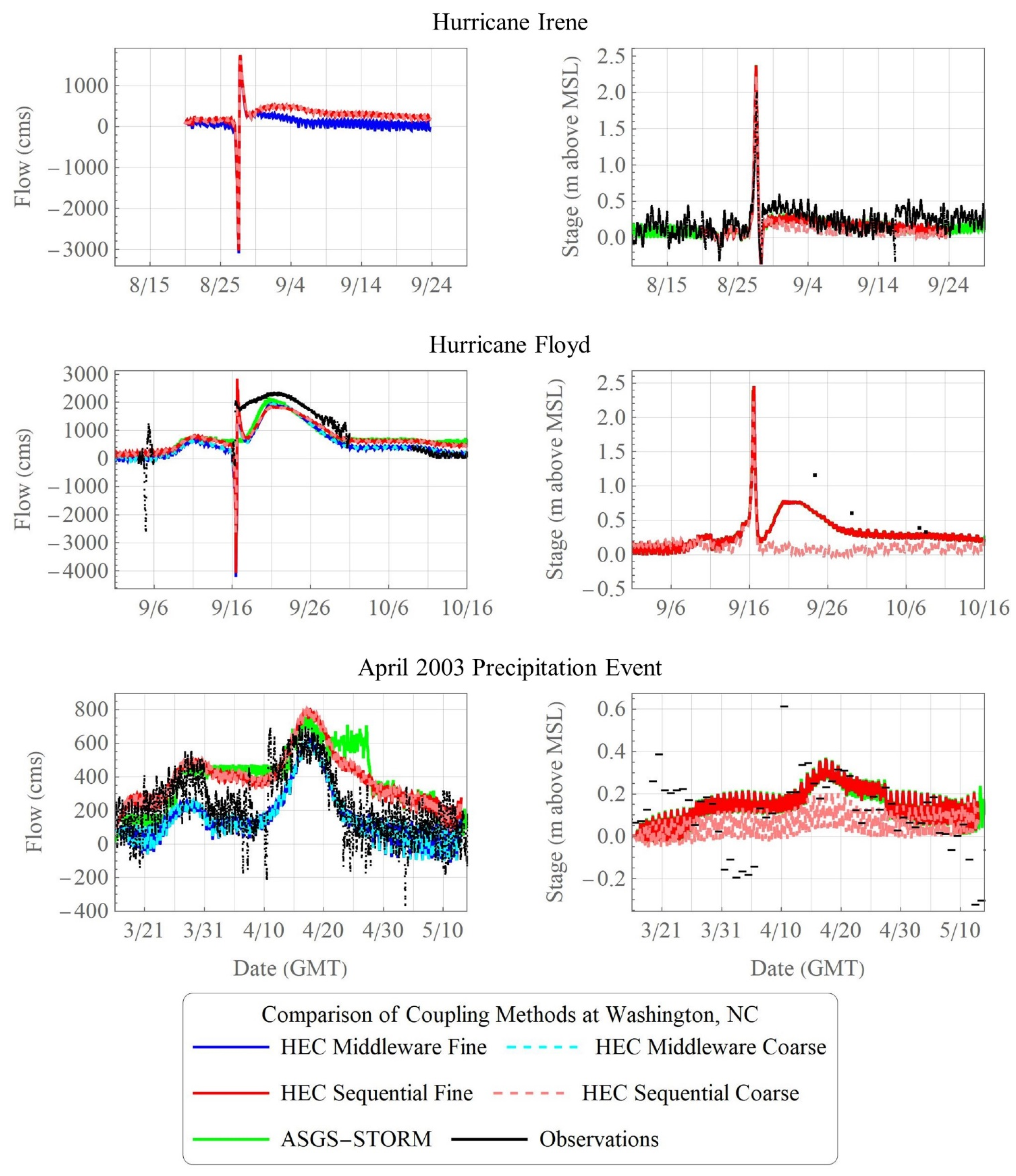
3.2. Influence of Boundary Conditions
To achieve an objective comparison of each coupling method, the error in the prescribed boundary conditions is examined. Specifically, model results are compared to observed flow and stage hydrographs collected on the Tar River at Tarboro, NC [
50], and Pamlico Sound at Washington, NC [
51,
52], near the HEC-RAS boundaries.
Figure 5 compares the modeled streamflow and stage for each event at the upstream boundary with observations taken at the Tarboro gauge (for reference, this gauge is located 2.8 m above NAVD88, and stage peaks at this point in the river are due to rainfall-runoff only). Recall that the sequential HEC-RAS (red) scheme is forced with the stage from the ASGS (green), which is why the stage is virtually identical for these coupling schemes at this upstream HEC-RAS boundary. Furthermore, we note that stages for these schemes consistently predict higher peaks while flows do not follow a consistent pattern. In general, the middleware HEC-RAS (blue) more accurately predicts peak flows and stages and better captures the receding limbs, but it estimates that peaks will occur earlier than was observed for Irene and Floyd. Additionally, while the middleware scheme does a fairly decent job of approximating the flows for all events, the stages are underpredicted for Floyd and the April 2003 event, indicating that there could be an error in the stage-discharge relationship within the HEC model. Finally, for all events, the sequential (stage-driven) HEC-RAS scheme overestimates the rising and falling flows and stages significantly, behavior which was also seen in the boundary verification study in
Section 2.3.2.
For the downstream HEC-RAS boundary shown in
Figure 6, we note that the USGS gauge at Washington did not record stages until 2007, so no data is available for Floyd, and it ceased recording streamflows in late 2006, so no flow data is available for Irene. For each event, the downstream stages that include riverine flow (fine ADCIRC) are higher than those that do not. We also note that this gauge is within the tidal portion of the river, indicating a definite need to force HEC-RAS with stages at the downstream boundary to accurately model the lower river. For example, note that the timing of the storm surge for both Irene and Floyd coincides with a complete flow reversal in all of the model results, as nearly 2 m of the extra stage is pushed upriver by the hurricane storm surge. Although the incorporation of rivers does not make much difference at this downstream location for Hurricane Irene, there is a considerable increase in stage for both Floyd and the April 2003 precipitation event. For Floyd, we note that the rainfall-induced stage peak occurs several days after the surge peak, and its effects linger for over a week.
Although the stages shown in the right panels are used as the lower river boundary condition for both HEC-RAS couplings, we note that there is not a significant change in the flow hydrographs for cases with versus without rivers during Floyd (as indicated by the lack of separation in the solid and dashed lines in the left panels). It is not as obvious whether this is true for the April 2003 event since it exhibits higher tidal variation; however, there is no change in the actual modeled flows for this event. Notice that the HEC-middleware approach best matches the leading and trailing streamflows for Floyd, while for the April 2003 event, the sequential HEC or existing ASGS schemes best capture the leading and peak flowrates but are too high during the trailing phase for both peaks (1–9 April and from 20 April on).
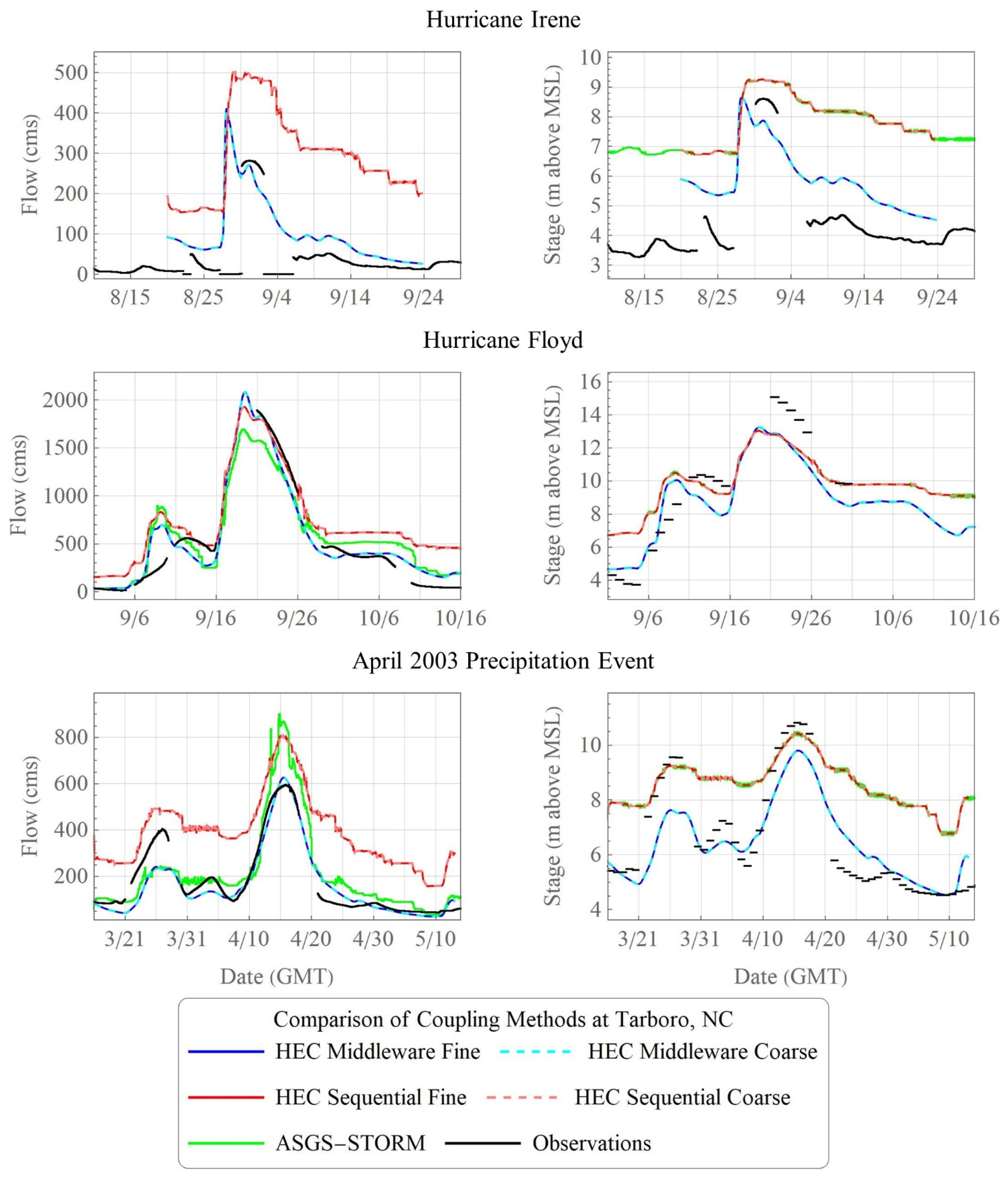
3.3. Interior Model Performance
Recall from
Figure 1 that there are three additional USGS gauges located along the Tar River within the interior domain of the HEC-RAS model: Rock Springs, Greenville, and Grimesland. For the timeline of these three events, both streamflows and stage are available at the central station located near Greenville. Additionally, stages are available at Rock Springs and Grimesland for only Hurricane Irene. Hydrographs for the common Greenville station are presented below in
Figure 7, and the additional gauges are discussed qualitatively for Irene.
Given that the error behavior remained relatively consistent at both boundaries (
Section 3.1), it comes as no surprise that these patterns repeat within the river model domain as well. Namely, the flow-driven HEC-RAS middleware (blue) best captures the overall flow rates for each event (peak and rising/falling limbs), while the existing ASGS does the best job of capturing peak stages, and the HEC-RAS middleware best matches falling limb stage behavior. For Floyd, we note that none of the coupling schemes are capable of capturing the observed peak stage, which indicates a resolution problem, i.e., the model rating curve does not faithfully represent the topology of the area. Notice also that at this station, there is no difference in HEC-RAS results (sequential or middleware) due to the “with or without” river stage downstream.
The stage results for Irene at Rock Springs and Grimesland follow the same trends as noted for Greenville, with one noticeable change: at this station, which is located near the downstream boundary, there are differences of up to 0.5ft in the stage due to the influence of river incorporation in the HEC-RAS downstream boundary condition.
For all events and stations, we note that the ASGS and sequential HEC-RAS schemes show an artificial “stair-step” pattern and fail to return to baseflow stages or flows during the falling limb stage. Additionally, the sequential (stage-driven) HEC-RAS tends to overestimate the actual streamflow. As noted in the other literature, this implementation of the ADCIRC model was not set up to capture baseflow but rather was designed to capture extreme flood effects. More specifically, even with the “fine” resolution, ADCIRC cannot capture subscale river morphology/geometry features, so at lower flows, the stage and discharge may be exaggerated, as compared to observations, and recession curves get pinned at artificially high levels. This was first reported by Tromble [
19] in his comparison of measured vs. model rating curves at various river stations. In the end, a compromise between model resolution and model efficiency was reached where the river features were resolved just enough to capture peak flows but not baseflow conditions.
Turning now to quantitative errors in magnitude and the timing of stage peaks for the coupling schemes,
Figure 8 shows these errors with respect to their distance along the river (the most downstream point at Washington going upstream to the right). For clarity, no errors are shown for the “no river” downstream condition since these changes were relatively small at most stations. The same color scheme is used to represent the coupling methods, while the shapes indicate which event is being considered.
Looking first at the errors in the peak stage, we note that near the downstream boundary, the errors are relatively small for all models, although data is sparse for these stations. As we progress upstream, we note that the ASGS (green) and sequential HEC-RAS (red) models typically have smaller peak stage errors when compared to the HEC-RAS middleware (blue) model. With regard to peak timing, there are significant errors for all upstream stations when using the HEC-RAS middleware approach, which is largely due to this being a flow-driven upstream boundary as opposed to stage-driven. Meanwhile, there are significant peak stage errors further upstream when using ADCIRC-upstream boundary conditions.
3.4. Comparison of Inundation Extents and Depths
To evaluate the inundation extents with the different coupling schemes, water surface elevation maps were developed from the peak elevations recorded from both the HEC-RAS and ASGS coupled models. Similar behavior was noted for all three events, as discussed below, so maps are only shown for Hurricane Floyd near Greenville (below in
Figure 9); the interested reader may view results for all three events in Bush [
49]. Note that the layers were ordered such that all three colors are visible, even if only by a few pixels.
For Irene, all three coupled models produced very similar inundation extents along the river, although the HEC-RAS coupling showed slightly smaller extents, particularly at more upstream locations. Although not shown herein, the ASGS coupling scheme generally results in deeper inundation depths than either of the HEC-RAS couplings, except for localized regions, e.g., upstream of bridges, which cause backwater effects that are not captured by ADCIRC at this scale and near tight meanders. For Floyd, the ASGS coupling produces slightly wider inundation extents than either of the HEC-RAS couplings, which are nearly the same, and again, the ASGS scheme results in slightly deeper inundation depths except for a small region near the upstream boundary at Tarboro. Finally, for the April 2003 precipitation event, we note that general inundation extent and depth trends followed the observations made for Hurricane Irene.
Additionally, we analyzed the effects of the downstream HEC-RAS boundary condition obtained from ADCIRC stages with and without river flows (coarse vs. fine ADCIRC). The differences in the final modeled HEC-RAS stage results, defined as inundation with rivers less without rivers, are shown in
Figure 10.
Note that for Irene and the April 2003 event, these differences are less than 15 cm near the downstream boundary and less than 3 cm by Greenville. Meanwhile, Floyd has a more significant difference, i.e., nearly 30 cm, in the upper sound but has less change in the river itself (the majority of the river has less than a 3 cm difference). However, we note that the HEC-RAS scheme was eight feet lower near Greenville when predicting the actual surge peak for this storm, which affects these inundation depths.
4. Summary
Ultimately, we are interested in comparing compound flooding simulated with HEC-RAS versus ADCIRC (ASGS system). For each of the storms, differences have been presented with qualitative (hydrograph shapes) and quantitative (peak surge and timing errors) measures, along with comparing inundation extents and depths. This research has attempted to answer the question, Does the use of an industry-standard hydraulic model, such as HEC-RAS, as so-called “middleware” between the hydrology and hydrodynamic models reduce runtimes without sacrificing the accuracy of a coupled modeling system, compared to a system that does not employ a river hydraulic model?
Turning first to the analysis of the hydrographs themselves, we note the following general observations.
HEC-RAS middleware does the best job of capturing streamflows for all locations and events and the best job of capturing pre- and post-surge stages (during lower flows).
HEC-RAS sequential and ASGS generally do the best job matching the peak stages, but both tend to over predict the base flows (and corresponding base stages).
HEC-RAS sequential provides hydrograph shapes that are more similar to those observed, especially on the receding limb, than ASGS alone, which tends to generate artificial stair-stepping due to the grid scale’s interaction with the wetting and drying algorithm; however, the sequential coupling does not necessarily improve the peak values themselves.
The impact of using with versus without river ADCIRC results for the downstream HEC-RAS middleware boundary condition is largely attenuated by Greensville and is more significant below Grimesland.
As a second comparison of the results presented above, we analyzed the downstream boundary conditions from the ADCIRC model for the HEC-RAS middleware scheme from a computational cost vs. benefit point of view. In particular, we evaluated whether there is a loss of accuracy in the HEC-RAS model due to the coarser ADCIRC model (lower cost) in the downstream boundary condition. We note the following general observations for all events.
Visible separation of the blue lines in the hydrographs was only evident at Grimesland.
Inundation depths were only significantly affected below Greenville (less than a cm above this location), with the most noticeable changes occurring closer to Grimesland (up to 15 cm) and within the sound itself (up to 30 cm for Floyd).
The finer ADCIRC model with riverine flows has an associated 50% increase in computational cost.
Given these increased computational costs and the localized nature of the area of influence, it does not appear to be beneficial to add the riverine flow via a fine ADCIRC model unless a very high degree of accuracy is required near the downstream HEC-RAS boundary.
Finally, it was hypothesized that simply coupling an existing HEC-RAS model to the ADCIRC model with a coarsely resolved riverine mesh would immediately enable river simulations, at a significant cost reduction, without reducing the accuracy of the modeling system. Given the observations above, we note that, unfortunately, this does not seem to be the case. Although there would be significant computational cost savings, the HEC-RAS middleware approach is most accurate at predicting streamflows and leading/trailing stages but less accurate when predicting peak inundation depths (stage). However, it should be noted that the ASGS riverine grid was not developed to capture low flow events; rather, it was developed specifically to capture extreme events and, thus, excels in that regard. By looking at both the qualitative and quantitative results, we can conclude that the results with either HEC-RAS coupling scheme show notable improvements in producing “realistic-looking” hydrographs but do not consistently show increased skill in predicting peak stages.
5. Conclusions and Future Work
In this manuscript, we have noted that the costs of the current model coupling scheme using ADCIRC are high, and the HEC-RAS middleware coupling shows potential but is not as accurate as the current ASGS scheme when determining peak stages. However, it is more accurate for baseflow conditions and leading/receding limb flows and stages. Therefore, there is no single ideal coupling scheme.
Currently, there is a significant error due to the presently available upstream boundary conditions from HL-RDHM. The presence of pre-storm overestimated baseflows in the ADCIRC boundary conditions suggests that baseflow errors may be related to the representation of the confluence zone (between Fishing Creek and the Tar River) between the ADCIRC HL-RDHM handoff point and the HEC-RAS HL-RDHM handoff point. Receding limb problems appear to be due to the interaction of the grid resolution with the wetting and drying algorithm in ADCIRC (details of which are discussed by Dick et al. [
59] and Tromble [
19] and typified by the use of a single-element-wide river). Greater resolution in the ADCIRC model or the inclusion of partial wetting and drying algorithms may produce more realistic falling-limb behavior in stage results derived from ADCIRC results.
This research indicates possible future studies in at least four areas: determination of the radius of impact of downstream boundary condition errors, development of more accurate boundary conditions, quantification of timing advantages of proposed couplings, and the impact of improved resolution in the river representation in the hydrodynamic model. Each of these is discussed in the paragraphs below.
The Tar River (as with all rivers with shallow bed slopes) is impacted by both upstream and downstream boundary conditions in varying ways. It is evident from the maps of inundation depth error associated with the downstream boundary condition (
Figure 10) that the spatial zone of influence can vary widely with changing event conditions. It remains to be seen if, with sufficient parameterization, functional guidance could be developed to estimate a storm surge prediction’s impact on stage predictions in terms of the distance upstream. If this “radius of impact” associated with resolved rivers in a 2D model could be established for all expected storm conditions, the implementation of this sort of middleware coupling would be rendered more predictable in terms of error behaviors. Furthermore, boundary conditions at the upstream edge of the riverine domain dominate the differences between the two HEC-RAS couplings. Additional attention to this boundary condition may reduce or eliminate the errors associated with the proposed scheme in the regions outside of the “radius of impact” of the downstream boundary.
The cost/benefit analysis presented in this manuscript used rough estimates to determine computational costs. A rigorous timing trial on operational-scale architectures may reveal more precisely the time costs associated with resolving rivers. If the quality of a proposed new coupling can be improved, then a more formal cost/benefit analysis can be produced that statistically accounts for the reduction in expected error associated with additional ensemble modeling members. In addition, this comparison did not formally examine the additional cost of developing the HEC-RAS model (as this work was performed by Abshire [
48]), nor did it examine the cost or workload of operating a third model as middleware, as the coupling implementation used here (single-event, non-dynamic coupling, with manually-passed data) would appear very different in a real-time operational scheme, ideally featuring automated data passing, perhaps with a dynamic coupling scheme.
Finally, the current study did not attempt to modify the resolution of the operational riverine mesh, as it was considered cost-prohibitive. However, given that there is always a tradeoff between simulation time and model accuracy, the development of a more finely resolved river model may justify the increased simulation cost if it produces a very high degree of predictive skill. For example, if costs per member double, but the resulting error envelope of an ensemble simulation with ½ the member size was reduced, increased resolution in the rivers will have justified the increased cost.


