Infrared and Visible Image Fusion Methods for Unmanned Surface Vessels with Marine Applications

Abstract

Infrared and visible image fusion is a very effective way to solve the degradation of sea images for unmanned surface vessels (USVs). Fused images with more clarity and information are useful for the visual system of USVs, especially in harsh marine environments. In this work, three novel fusion strategies based on adaptive weight, cross bilateral filtering, and guided filtering are proposed to fuse the feature maps that are extracted from source images. First, the infrared and visible cameras equipped on the USV are calibrated using a self-designed calibration board. Then, pairs of images containing water scenes are aligned and used as experimental data. Finally, each proposed strategy is inserted into the neural network as a fusion layer to verify the improvements in quality of water surface images. Compared to existing methods, the proposed method based on adaptive weight provides a higher spatial resolution and, in most cases, less spectral distortion. The experimental results show that the visual quality of fused images obtained based on an adaptive weight strategy is superior compared to other strategies, while also providing an acceptable computational load.

1. Introduction

Recently, USVs have received considerable attention due to their high working efficiency and strong adaptability in ocean missions, such as maritime search and rescue, port surveillance, and ocean environment monitoring [1,2,3]. To make USVs competent for these mission requirements, object detection and recognition are of the utmost significance for them to sense the surrounding environment. However, due to the complex working environment, there are still various obstacles to achieving satisfactory environment recognition performance on the sea surface, such as sea fog, sea reflections, and rainstorms [4].

To sense the environment more clearly, fusing infrared and visible images is superior in many aspects [5]. First, a USV will generally be equipped with an optoelectronic device to capture visible and infrared images at the same time, making this method easy to implement [6,7,8,9,10]. Second, infrared and visible images provide scene information from different aspects. Data from images at different frequencies are combined to enhance the knowledge obtained from expected scene information. This combination contains more information than the combination of single-modality signals [11]. Finally, infrared and visible images have complementary characteristics, which means that fused images are robust and informative. Visible images typically have a high spatial resolution and considerable detail and chiaroscuro, but they will be seriously degraded in severe weather [12,13,14], while infrared images, which depict the information of objects from a different aspect, are resistant to these disturbances at lower resolutions. Fusion technology can combine the advantages of these two kinds of images to obtain better results. Therefore, it is highly preferable to incorporate infrared and visible image fusion techniques in environmental perception to enhance the adaptability of USVs. It is worth noting that, due to its applicability in all conditions and even in high-humidity environments, medium-wave infrared (MWIR) cameras that are sensitive to a thermal energy of 3–5 μm are generally used on USVs. Thus, only medium-wave infrared was considered in this study.

Many researchers have studied the fusion of infrared and visible images and provided different methods [5]. Multi-scale transform-based methods have proven to be very effective for image fusion and other image-processing tasks [15,16,17]. A multi-scale representation of the input image is obtained by multi-scale transformation. The multi-scale coefficients of fusion are obtained according to specific fusion rules, which usually take into account the activity of the coefficients and the correlation between adjacent pixels or pixels of different scales. Finally, the fusion coefficients are inversely transformed to obtain the fused image. This image fusion framework involves two basic problems, the choice of the multi-scale decomposition method or the fusion strategy for multi-scale coefficient fusion. Sparse representation [18,19,20,21,22] has emerged as a novel signal analysis model, where the signal can be expressed as a linear combination of a few atoms that can reveal the intrinsic properties of the image. The representation of images with linear combinations of sparse bases is the key to their good performance.

In recent years, with advances in computer performance, neural network theory has been further improved [23,24]. Neural network-based methods have better real-time performance and effectiveness compared to other methods, so they are suitable for USVs. Liu et al. [25] proposed a fusion method based on convolutional sparse representation (CSR), in which two raw images are taken as input to the network, and the extracted feature details based on CSR are considered to obtain a fused image. This method is more stable than the fusion method based on sparse representation. After that, Liu et al. [26] presented a CNN-based fusion method for the task of multi-focus image fusion. This CNN-based approach encodes direct mapping from source images to weight maps so that the activity level measurement and weight assignment can be obtained directly by training the neural network. However, this method can only be used in multi-focus image fusion. Wu et al. [27] used the L1 norm and weighted-average strategy to generate several candidates for fused detail content, with features extracted by a deep learning network. The fused image is reconstructed by combining the fused base part and the detail content. However, these neural network-based methods only use the features extracted from the last layer in the neural network, which results in the loss of shallow feature information obtained in the process of feature extraction. To overcome this drawback, Wu et al. [28] presented a novel deep learning architecture named DenseFuse for infrared and visible image fusion. The encoding network is combined by convolutional networks, fusion layers, and dense blocks, in which the output of each layer is connected to every other layer. It can avoid losing the feature information in the middle layer by making more effective use of the features extracted from the original image. However, the inputs are fused according to the two fusion strategies, in which feature maps from different sources have the same importance. As a result, the complementarity of the two images cannot be effectively utilized.

Motivated by the above observations, this paper provides three fusion strategies to improve the image fusion quality for USVs under complicated sea environments. Contributions of this work are summarized as follows:

(1)

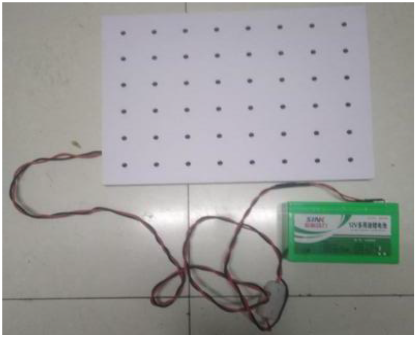
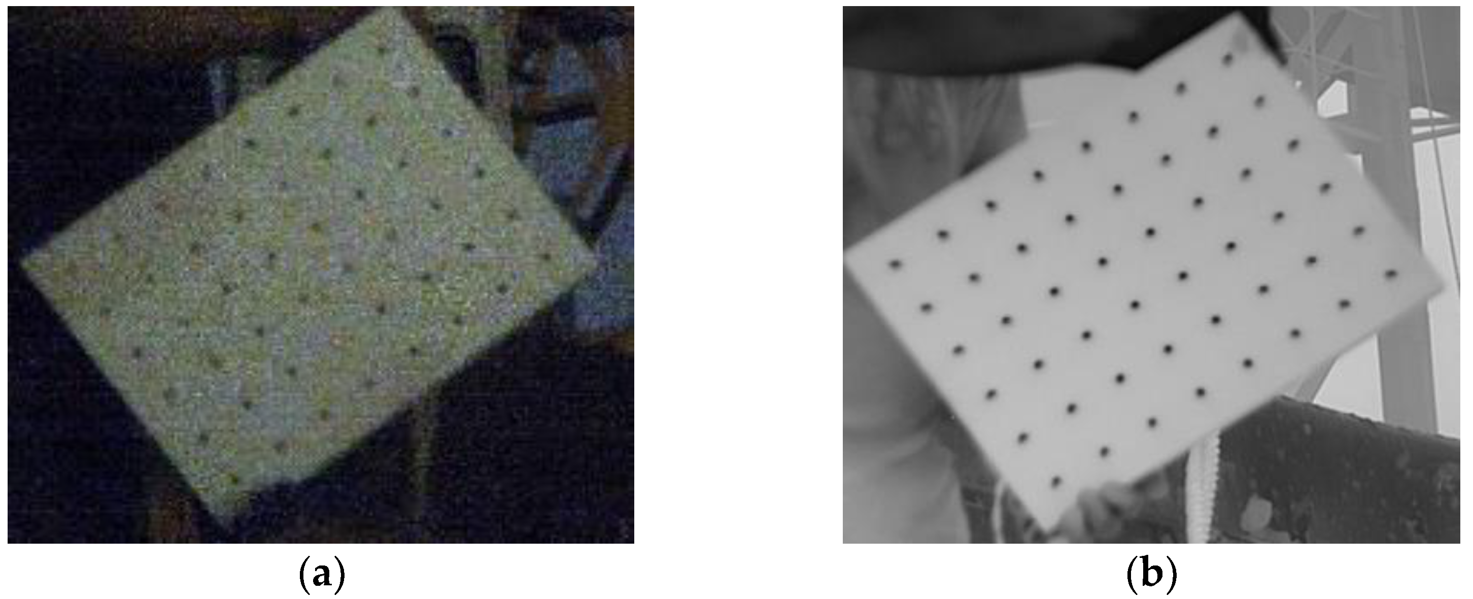
A novel calibration board was designed to calibrate infrared and visible cameras. To avoid the loss of detailed texture in infrared images that is induced by the thermal diffusion between high- and low-temperature regions, all heating elements of the calibration board are processed to be insulated, which makes the accuracy of the calibration able to be improved. Moreover, a major part of the calibration board is made of lightweight thermal insulation material. Thus, the designed calibration board not only possesses high contrast for both visible images and infrared images, but it also enjoys high portability in USV field applications.

(2)

Three novel fusion strategies, adaptive weight fusion (AWF), cross bilateral filtering fusion (CBF), and guided filtering fusion (GFF), are proposed in this paper. The AWF calculates the weight of each sub-block, rather than roughly calculating the feature maps’ weights, such that the fusion result can be more accurate. The CBF considers intensity re-semblance and geometric closeness for the computation of fusion weights. The GFF utilizes a guided filter for edge preservation in the fusion results. Compared to the previous fusion strategies [28,29], the proposed fusion strategies make more effective use of the texture features in infrared images.

(3)

The proposed algorithms are compared with two widely accepted algorithms, average weighted fusion (AVE) [29] and L1 norm weighted fusion (L1) [28], under the optoelectronic system of ‘Tianxing-1’ USV. The experiment results indicate that the proposed AWF strategy can be applied to the USV and show superior performance on water surface images.

The paper is structured as follows: Section 2 introduces the self-designed calibration board used for camera calibration which is a precondition for infrared and visible image fusion. The proposed methods are explained in detail in Section 3. Section 4 presents the experimental results and a discussion. The paper concludes with Section 5.

2. Camera Calibration

In this study, a calibration board (shown in Figure 1) was designed to calibrate infrared and visible cameras. To generate the characteristics of infrared radiation, the calibration board contained 48 holes arranged in a 6 × 8 array, with a heating element in each hole. The horizontal and vertical distance between heating elements was 40 mm. To avoid the loss of detailed texture in infrared images due to thermal diffusion between high- and low-temperature regions, we used LED lights wrapped in black tape as heating elements. The base of the calibration board was made of insulation material so that the contrast of infrared images can be improved. The image information of the calibration board could be collected by the visible and infrared cameras simultaneously when the LED lights were on. Compared to the commonly used checkerboard, the calibration board is suitable for USV field tests, as it is more portable.

We captured visible and infrared images of the calibration board simultaneously, as shown in Figure 2. Following the method in the literature [30], the intrinsic parameters of the visible and infrared cameras and the extrinsic parameters between the two cameras can be estimated. In this way, we can extract the corresponding corner from the visible and infrared images simultaneously by using the calibration board.

After the camera calibration was completed, the visible and infrared images could be registered using the estimated parameters. The result is shown in Figure 3, which shows the superposition of visible gray image and infrared image. By observing this result, it can be concluded that the scene of the visible image is consistent with the infrared image. Therefore, the objects in these two figures are well aligned.

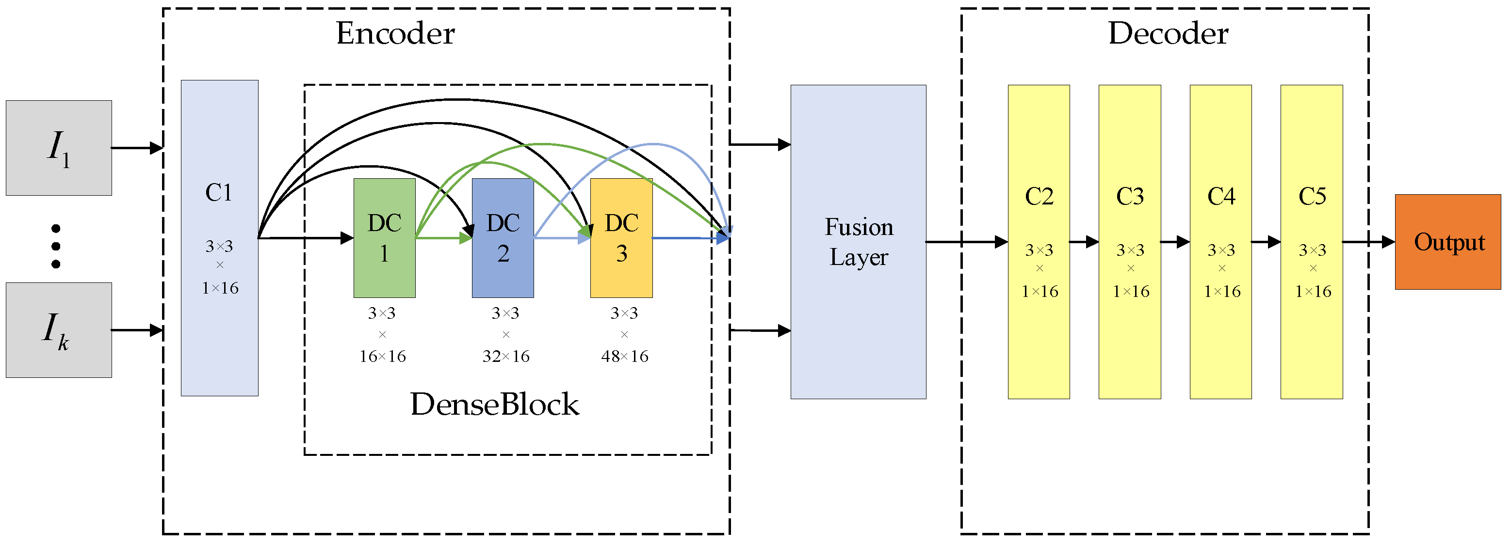
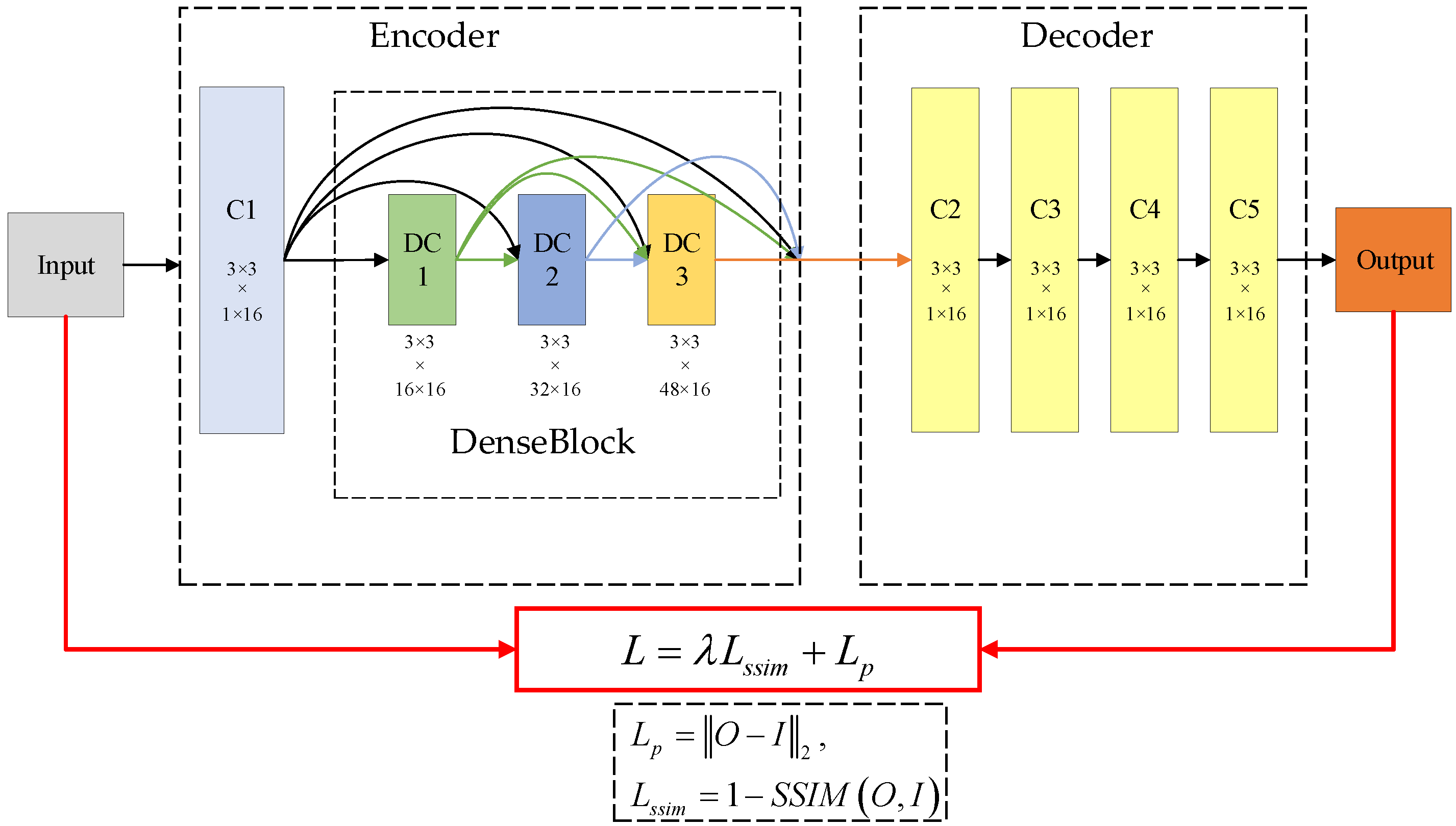
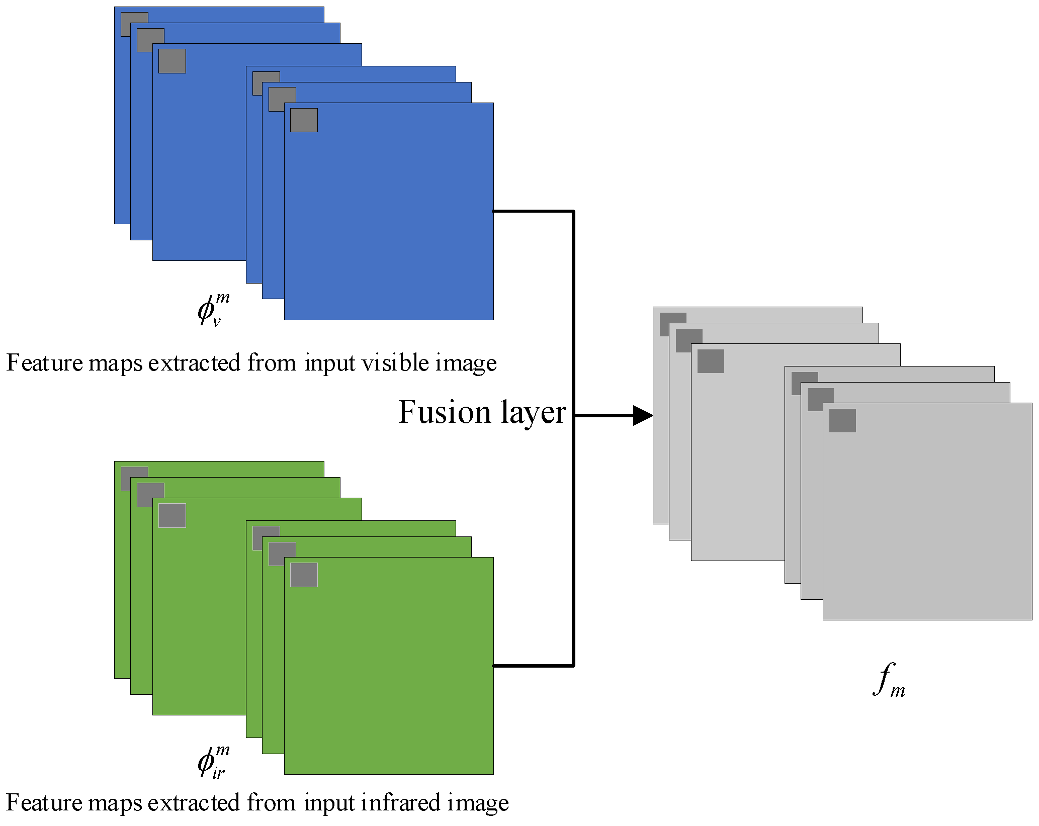
3. Improvement of Fusion Network

As shown in Figure 4, the detail framework of the network in [28] consisted of three parts: encoder, fusion layer, and decoder. The feature maps obtained by the encoder were fused in the fusion layer then were integrated into one feature map that contains all salient features in source images. Finally, the fused image was reconstructed by a decoder network.

The input images, including infrared and visible images, are denoted as $I_1,\dots ,I_k$, and $k\ge 2$. Note that the input images were registered in the process of camera calibration. As shown in Figure 4, the encoder consisted of a convolutional layer (C1) and a DenseBlock that contains three convolutional layers. The architecture of the DenseBlock can preserve deep features as much as possible in the encoding network.

In the training phase, the fusion layer was discarded, and only one image was fed into the network at a time. The loss function $L$ is a weighted combination of pixel loss $L_P$ and structural similarity (SSIM) loss $L_{ssim}$, with the weight $\lambda$ as shown in Figure 5. The pixel loss $L_P$ indicates the Euclidean distance between the output $O$ and the input $I$. The $SSIM(·)$ in $L_{ssim}$ denotes the structural similarity of two images. The $\lambda$ was set as 1, 10, 100, and 1000, respectively, because there are three orders of magnitude differences between $L_P$ and $L_{ssim}$. Based on the above, the encoder and decoder network can be trained to reconstruct the input image. The detailed framework of the network in the training phase is shown in Figure 5. The architecture of the network is outlined in

Table 1. Architecture of the training process. Conv, convolutional block consisting of a convolutional layer and an activation layer; Dense, DenseBlock.

	Layer	Size	Stride	Channel (Input)	Channel (Output)	Activation
Encoder	Conv (C1)	3	1	1	16	ReLU
	Dense
Decoder	Conv (C2)	3	1	64	64	ReLU
	Conv (C3)	3	1	64	32	ReLU
	Conv (C4)	3	1	32	16	ReLU
	Conv (C5)	3	1	16	1	ReLU
Dense (DenseBlock)	Conv (DC1)	3	1	16	16	ReLU
	Conv (DC1)	3	1	32	16	ReLU
	Conv (DC1)	3	1	48	16	ReLU

.

When the network has the ability to reconstruct the input images, the quality of the fusion result depends on the fusion layer (strategy). The fusion layer is used to combine the salient feature maps from different sources. The final fused image is obtained by the decoder, in which the result of the fusion layer is regarded as the input. A diagram of the fusion layer is shown in Figure 6.

Different from [28], which focused on the feature extraction and reconstruction ability of the neural network, the fusion strategy in the neural network was further studied in this study. Two fusion strategies (AVE, L1) used for the network were proposed in [28]. The AVE takes the average sum of two feature maps as the fusion result. The L1 calculated the value of the L1 norm between two feature maps as the fusion weight. It was proven that the L1 norm strategy had better performance, but it still has shortcomings that could be improved. In the L1 norm strategy, the weighted sum of feature maps is used to achieve the fusion of feature maps, in which the weight is set for the entire feature map. The interaction between different parts within the feature map is not considered. Moreover, the L1 norm strategy only calculates the values in the 3 × 3 range around the point, which leads to the loss of the remaining features. To make up for these drawbacks, we proposed three novel fusion strategies to improve the quality of the fusion result by improving the fusion layer (strategy) in the network.

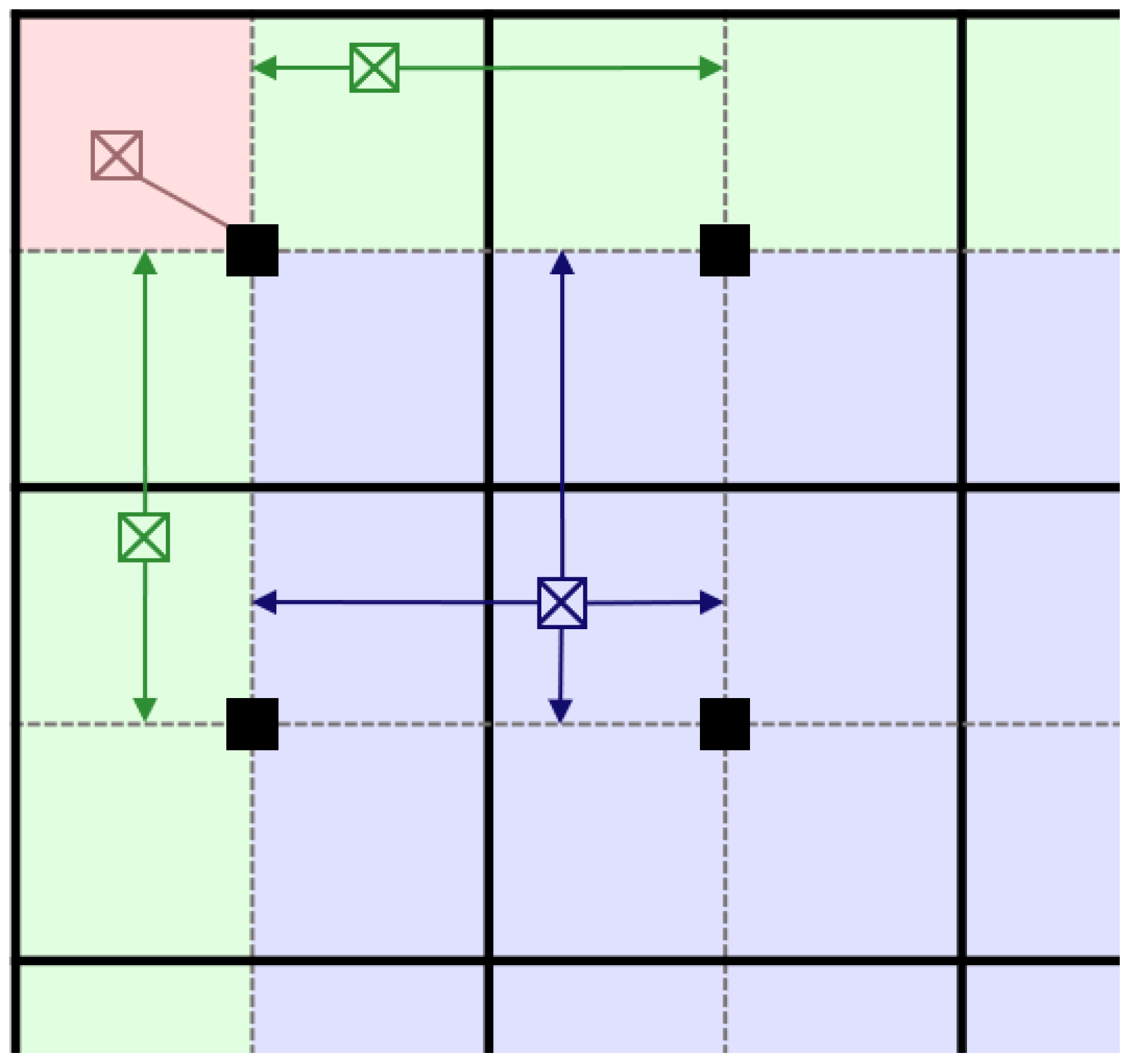
3.1. Adaptive Weight Strategy

In this section, the adaptive weight-based fusion (AWF) strategy is developed. The visible and infrared feature maps are divided into blocks, with AWF utilized by the window size $l\times l$ (better result with $l=80$). The weights are calculated for the blocks rather than the whole feature map, resulting in a more accurate fused feature map. In this way, feature loss is avoided, since the perceptual area corresponding to each point is increased.

If we define $D_{i.j}$ as the block located in row $i$, column $j$ within the feature map, then the corresponding weight $C_{i,j}({\varphi }^m)$ of block can be formulated as:

$$C_{i,j}({\varphi }^m)={\Vert {\varphi }^m(x^{\prime },y^{\prime })\Vert }_1,(x^{\prime },y^{\prime })\in D_{i,j}$$

(1)

where ${\varphi }^m\left(m\in \left\{1,\dots ,M\right\}\right)$ represents the feature maps extracted from one input image, with $M$ representing the number of feature maps, and $\left(x^{\prime },y^{\prime }\right)$ denotes the coordinates of any point in block $D_{i.j}$.

Then, the bilinear interpolation method was adopted to deal with the region segmentation problem induced by the blocking artifact. For any point $\left(x,y\right)$ in a feature map, the weights of its nearest four neighbor blocks are denoted as $C_{i,j},C_{i+1,j},C_{i,j+1},C_{i+1,j+1}$. For these blocks, we adopted the following method to set the weights of the point:

$$\begin{array}{cc}\hfill {\omega }^m(x,y)& =(1-\Delta y)((1-\Delta x)C_{i,j}({\varphi }^m)+\Delta x{C}_{i+1,j}({\varphi }^m))+\hfill \\ & \Delta y((1-\Delta x)C_{i,j+1}({\varphi }^m)+\Delta x{C}_{i+1,j+1}({\varphi }^m))\hfill \end{array}$$

(2)

where $\Delta x=\left|x-x_0\right|/l,\Delta y=\left|y-y_0\right|/l$, $\left(x_0,y_0\right)$ denotes the center of the upper left block. Then, the fusion feature map was generated by weighting the visible and infrared feature map according to the following formula:

$$f_m(x,y)=\frac{{\omega }_v^m(x,y)\times {\varphi }_v^m(x,y)+{\omega }_{ir}^m(x,y)\times {\varphi }_{ir}^m(x,y)}{{\omega }_v^m(x,y)+{\omega }_{ir}^m(x,y)}$$

(3)

where ${\varphi }_v^m\left(x,y\right)$ indicates feature maps of visible image and ${\varphi }_{ir}^m\left(x,y\right)$ for those of infrared image, as shown in Figure 6; ${\omega }_v^m(x,y)$ indicates the weight of ${\varphi }_v^m(x,y)$, and ${\omega }_{ir}^m\left(x,y\right)$ indicates the weight of ${\varphi }_{ir}^m\left(x,y\right)$. $\left(x,y\right)$ denotes the coordinates of any point in the feature map.

For a position in the edge area (green area in Figure 7), the weight at the corresponding points in the feature map is obtained by linear interpolation between two adjacent blocks. For a position in the corner area (pink area in Figure 7), the weight of this block is directly used as the weight of the point corresponding to the feature map.

The experimental results of the presented adaptive weight strategy are shown in Figure 8.

3.2. Cross Bilateral Filtering

Cross bilateral filtering (CBF) is a modified weight estimation method inspired by the bilateral filter [31]. This method considers both levels of gray similarities and the geometric closeness of neighborhood pixels in image A to adjust the filter kernel and filters the image B. The weights are computed by measuring the strength of the details in the detail image obtained by CBF. This method smoothens the image by preserving the edges and applying neighborhood pixels. Therefore, this method makes better use of the texture details in the infrared image than the fusion strategy in [28], which directly takes L1 parameters as fusion weights. Note that the structural similarity between feature maps extracted from infrared and visible images meets the application conditions of CBF.

(1)

CBF

The feature maps of infrared images were used to filter the corresponding feature maps of visible images. To simplify the expression, $A$ denotes the ${\varphi }_{ir}^m$, and $B$ denotes the ${\varphi }_v^m$. The CBF output of B marked as $B_{CBF}$ at pixel location $p$ is calculated as:

$$B_{CBF}=\frac{1}{W}{\displaystyle \sum _{q\in S}{G}_{{\sigma }_s}}\left(\Vert p-q\Vert \right)\times G_{{\sigma }_r}\left(\left|A\left(p\right)-A\left(q\right)\right|\right)B\left(q\right)$$

(4)

$$W={\displaystyle \sum _{q\in S}(\exp (-\frac{{\Vert p-q\Vert }^2}{2{\sigma }_s^2})\exp (-\frac{{\Vert A(p)-A(q)\Vert }^2}{2{\sigma }_r^2})}$$

(5)

where $G_{{\sigma }_s}\left(\Vert p-q\Vert \right)=e^{-\frac{{\Vert p-q\Vert }^2}{2{\sigma }_s{}^2}}$ represents a geometric closeness function with the design parameter ${\sigma }_s$, which is normally set to 1.8; $\Vert p-q\Vert$ is the Euclidean distance between $p$ and $q$; $G_{{\sigma }_r}\left(\left|A\left(p\right)-A\left(q\right)\right|\right)=e^{-\frac{{\left|A\left(p\right)-A\left(q\right)\right|}^2}{2{\sigma }_r{}^2}}$ is a gray-level similarity edge stopping function, ${\sigma }_r$ is a design parameter which is normally set to 25, $A(·)$ denotes the pixel value at position $·$ in feature map A and $B(·)$ in feature map B, and $S$ is the spatial neighborhood of $p$. $W$ is a normalization constant.

The detail image of feature maps $A$ and $B$ can be expressed with $A_D$ and $B_D$, respectively.

$$\begin{array}{l}{A}_D=A-A_{CBF}\\ B_D=B-B_{CBF}\end{array}$$

(6)

(2)

Pixed-based fusion rule

A window of size $l\times l$ (referring to [31], $l=11$) around a detail coefficient $A_D\left(x,y\right)$ or $B_D\left(x,y\right)$ is considered as a neighborhood to compute its weight. This neighborhood is denoted as matrix $M$. Each row of $M$ is treated as an observation and each column as a variable to compute the unbiased estimate ${ƛ}_{x,y}^h$ of its covariance matrix, in which $\left(x,y\right)$ are the spatial coordinates of the detail coefficient $A_D\left(x,y\right)$ or $B_D\left(x,y\right)$.

$$\mathrm{cov}\left(M\right)=E\left[\left(M-E\left[M\right]\right){\left(M-E\left(M\right)\right)}^T\right]$$

(7)

$${ƛ}_{x,y}^h=\frac{{\displaystyle \sum _{k=1}^l(x_k-\overline{x})(x_k-\overline{x}}{)}^T}{l-1}$$

(8)

where $x_k$ is the kth observation of the $l$-dimensional variable, and $\overline{x}$ is the mean of observation. Similarly, an unbiased covariance estimate ${ƛ}_{x,y}^v$ is computed by treating each column of $M$ as an observation and each row as a variable (opposite to that of ${ƛ}_{x,y}^h$). The sum of these eigenvalues is directly proportional to the horizontal detail strength of the neighborhood and is denoted as $S_h$. Similarly, the sum of eigenvalues of ${ƛ}_{x,y}^v$ gives vertical detail strength $S_v$. That is,

$$S_h(x,y)={\displaystyle \sum _{k=1}^{l}eige{n}_k} of {ƛ}_{x,y}^h$$

(9)

$$S_v(x,y)={\displaystyle \sum _{k=1}^{l}eige{n}_k} of {ƛ}_{x,y}^v$$

(10)

where $eige{n}_k$ is the $k\mathrm{th}$ eigenvalue of the unbiased estimate of the covariance matrix.

The addition operation between horizontal detail strength $S_h$ and vertical detail strength $S_v$ can lead to the weight of a particular detail factor:

$$wt\left(x,y\right)=S_h(x,y)+S_v(x,y)$$

(11)

Therefore, the fused feature map is computed using the following equation:

$$f_m(x,y)=\frac{A\left(x,y\right)w{t}_a\left(x,y\right)+B\left(x,y\right)w{t}_b\left(x,y\right)}{w{t}_a\left(x,y\right)+w{t}_b\left(x,y\right)}$$

(12)

where the weights for the detail coefficient $A_D$ and $B_D$ are denoted as $w{t}_a$ and $w{t}_b$.

The results of the fusion strategy based on CBF are shown in Figure 9.

3.3. Guided Filtering

In this section, we improved the feature fusion layer using the guided filtering method [32], which acted as the DenseFuse network fusion rule. The L1 norm strategy in [28] calculated the L1 parametric number for both visible and infrared feature maps, resulting in them having the same importance in the algorithm. However, the texture features of infrared images were much clearer than those of visible images in actuality. Motivated by this, the fused feature map was reconstructed utilizing feature maps of infrared images ${\varphi }_{ir}^m$ to guide that of visible images ${\varphi }_v^m$, so that the textural features in the infrared images would be fully utilized in this fusion strategy.

We assume that $f_m$ is a linear transform of ${\varphi }_{ir}^m$ in a window $w_k$ centered at pixel k:

$$f_m\left(x,y\right)=a_k{\varphi }_{ir}^m\left(x,y\right)+b_k,\left(x,y\right)\in w_k$$

(13)

where $\left(a_k,b_k\right)$ are some linear coefficients assumed to be constant in $w_k$. This local linear model ensures that $f_m$ has an edge only if ${\varphi }_{ir}^m$ has an edge. In other words, the output will reflect the approximate contour edge of the guide. It is supposed that the output $f_m$ consists of input ${\varphi }_v^m$ and noise $n$.

$$f_m={\varphi }_v^m-n$$

(14)

Then, the following cost function was used to minimize the difference between $f_m$ and ${\varphi }_v^m$ while maintaining the linear model:

$$E(a_k,b_k)={\displaystyle \sum _{(x,y)\in w_k}\left({\left(a_k{\varphi }_{ir}^m\left(x,y\right)+b_k\right)}^2+\epsilon a_k^2\right)}$$

(15)

where $\epsilon$ is a regularization parameter penalizing large $a_k$. Equation (15) is the linear ridge regression model, and its solution is given by

$$a_k=\frac{\frac{1}{\left|w\right|}{\displaystyle \sum _{\left(x,y\right)\in w_k}{\varphi }_{ir}^m\left(x,y\right){\varphi }_v^m\left(x,y\right)-{\mu }_k\overline{{\varphi }_v^m\left(k\right)}}}{{\sigma }_k^2+\epsilon }$$

(16)

$$b_k=\overline{{\varphi }_v^m\left(k\right)}-a_k{\mu }_k$$

(17)

where ${\mu }_k$ and ${\sigma }_k^2$ are the mean and variance of $I$ in $w_k$, $\left|w\right|$ is the number of pixels in $w_k$, and $\overline{{\varphi }_v^m\left(k\right)}$ is the mean of ${\varphi }_v^m$ in $w_k$. After computing $\left(a_k,b_k\right)$ for all windows $w_k$ in the image, the filtering output was computed by

$$\begin{array}{c}{f}_m(x,y)=\frac{1}{\left|w\right|}{\displaystyle \sum _{\left(x,y\right)\in w_k}\left(a_k{\varphi }_{ir}^m+b_k\right)}\\ ={\overline{a}}_i{\varphi }_{ir}^m\left(x,y\right)+{\overline{b}}_i\end{array}$$

(18)

where ${\overline{a}}_i=\frac{1}{\left|w\right|}{\displaystyle \sum _{k\in w}{a}_k},{\overline{b}}_i=\frac{1}{\left|w\right|}{\displaystyle \sum _{k\in w}{b}_k}$.

A fusion strategy based on guided filtering can take advantage of the similarities between feature maps extracted from different sources. This method can preserve the edge contours and texture feature information of source images. The results are shown in Figure 10.

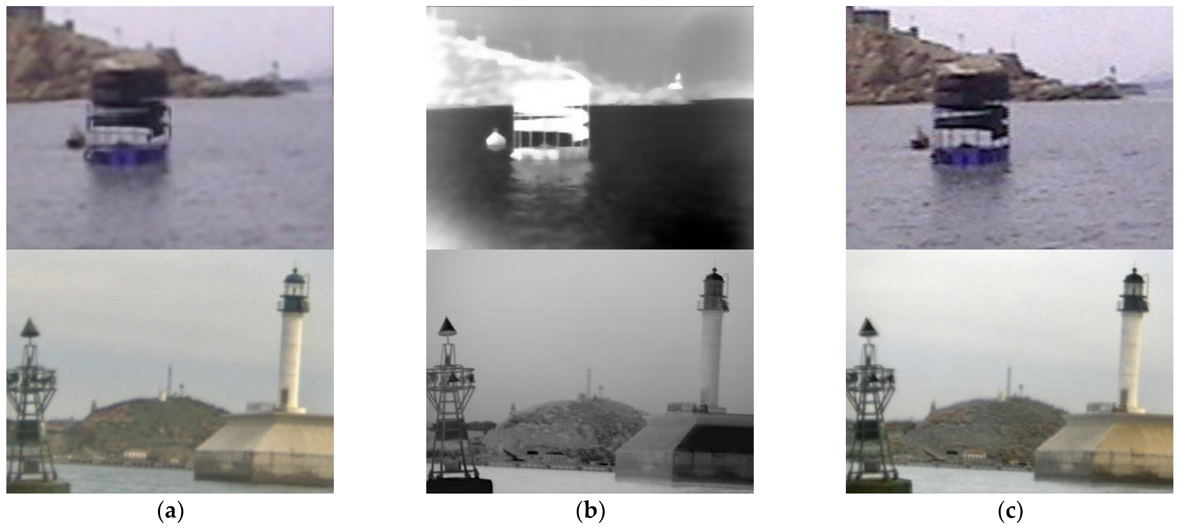
4. Experimental Results and Analysis

The results of the field experiments are given in this section to show that our proposed algorithm can improve the quality of sea images and is suitable for the USV visual system. We first trained the network to reconstruct the input images (fusion layer was discarded). The MS-COCO dataset was adopted to train the encoder and decoder network. In the dataset, about 79,000 images were utilized as input images, while the remaining 1000 images were used to validate the reconstruction ability. After the training, the parameters of the encoder and decoder were no longer updated. The fusion effect of different fusion strategies was observed by the improved fusion layer in the network.

To demonstrate the effectiveness and superiority of the proposed methods under other operating scenarios, we evaluated previous fusion methods (AVE, L1) and the proposed fusion method (AWF, CBF, GFF) in both qualitative and quantitative aspects. Eight representative pairs of visible and infrared images were selected, which were specified by different illumination contained by common sea scenes, such as coast, buoy, ship, and lighthouse. The ocean surface infrared images used in the experiment were collected with an MWIR camera equipped on the USV. The ‘Tian Xing’ USV platform for the experiment is shown in Figure 11.

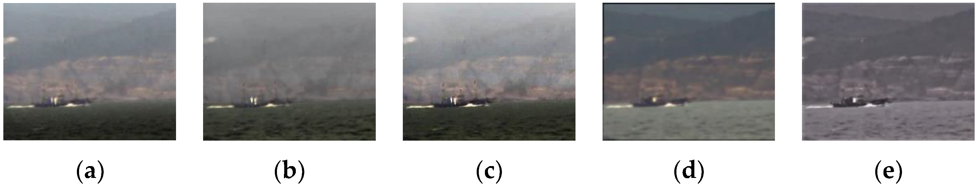
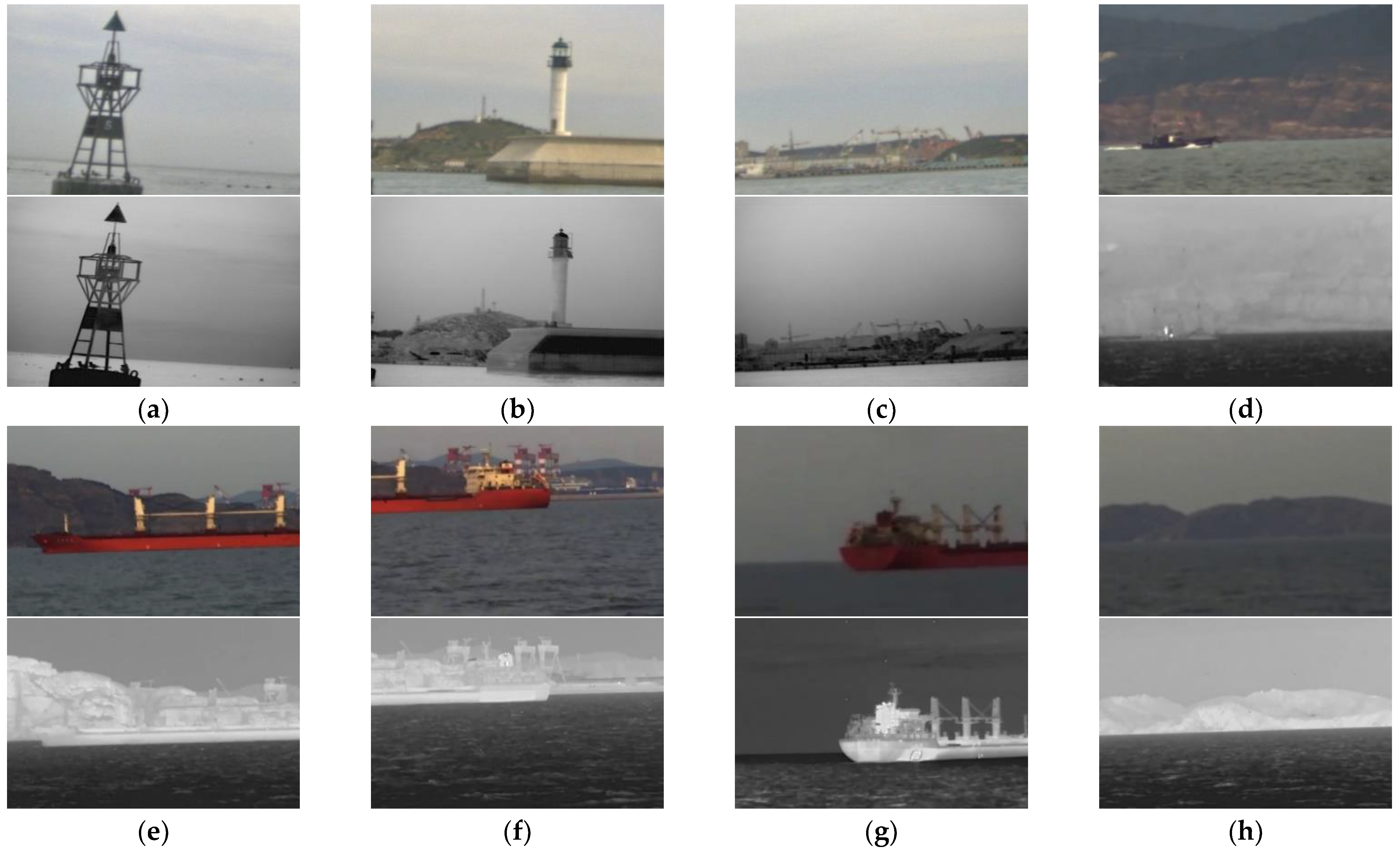
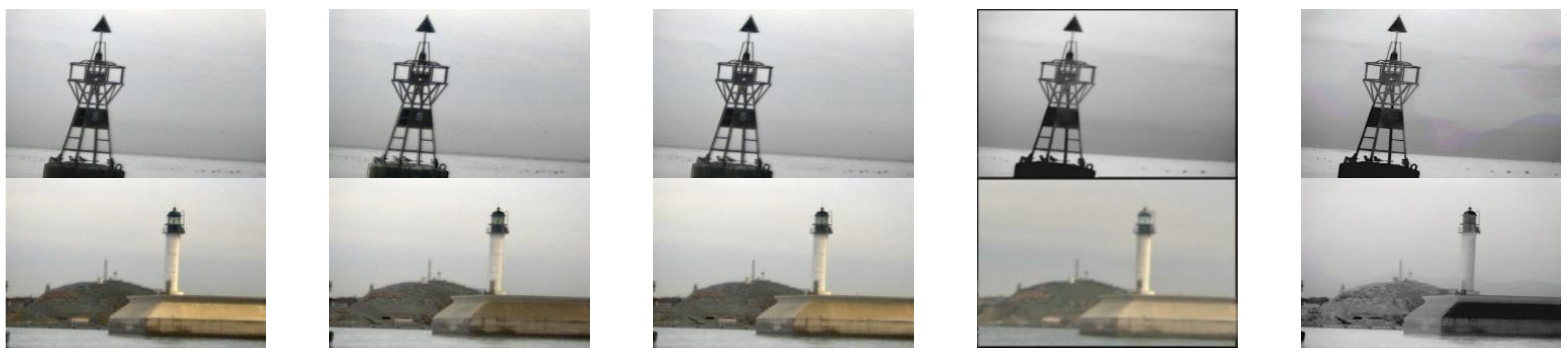
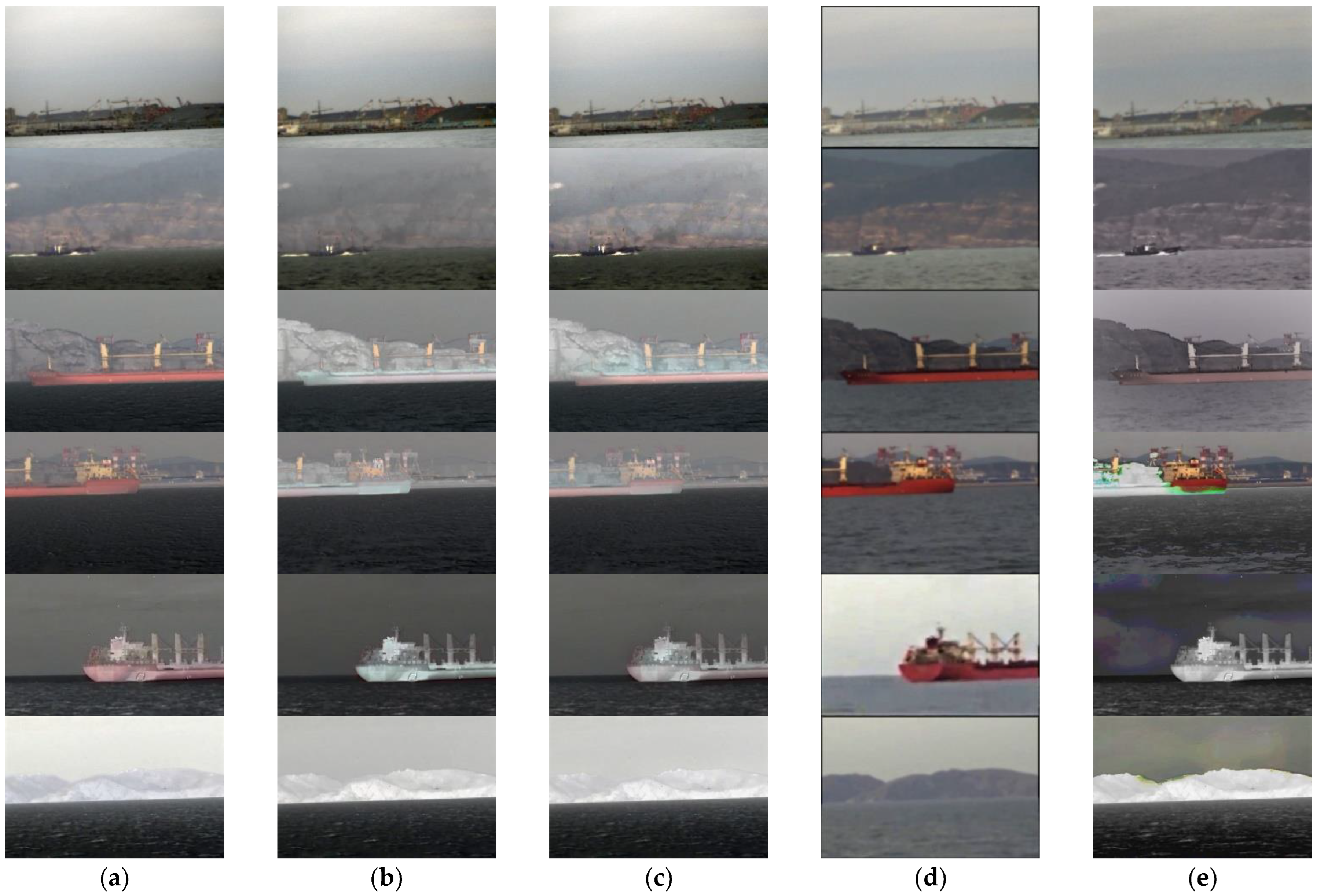
4.1. Qualitative Image Quality Assessment

The fusion results of the five algorithms are shown in Section 4.2. Our results seem to indicate that AWF had the best performance in clarity and contrast restoration, making the fused image look like a natural image. The fused image obtained by CBF had a complete scene structure, but the clarity was poor and the details of dense edge texture areas such as hillsides were poorly preserved. It did not have advantages over other methods. The contrast and clarity of the fused image obtained by GFF were better than the other methods. The details were clear, the texture details were retained completely, and the noise elimination effect was good. Distant ships, buoys, lighthouses, and other target objects could be clearly identified. However, the results show that there will be obvious color distortion under certain circumstances, which affects the overall image quality. In general, the proposed AWF fusion strategy had better performance under different working conditions.

4.2. Quantitative Image Quality Assessment

Quantitative image quality assessment can overcome the influence of subjective factors of the observer and make accurate and objective judgments on the effect of the image. The performance of proposed methods was evaluated in the following two aspects.

(1)

Quantitative assessment compared to baselines

To illustrate the effectiveness of the proposed three methods, they were compared with the AVE [29] and L1 in [28]. Comparison results of the three proposed methods with the AVE method and L1 method are given in Figure 12. For these results, the average gradient (AG) was adopted to measure the quality of the fusion result.

Assessments of the comparison results are summarized in

Table 2. Average gradient of fusion results.

	AVE	L1	AWF	CBF	GFF
Average gradient	1.063	0.957	1.121	1.195	1.092
Percentage change for AVE	-	-	+5.5%	+12.4%	+2.7%
Percentage change for L1	-	-	+14.9%	+22.6%	+12%

. From these results, we can observe that the presented methods (i.e., AWF, CBF, GFF) possessed higher AG values than the AVE and L1 method. To be specific, compared with the AVE and L1 method, the AG value improved by 5.5% (AWF), 12.4% (CBF), and 2.7% (GFF); 14.9% (AWF), 22.6% (CBF), and 12% (GFF), respectively. These results indicate that the three proposed methods had better performance in feature fusion than the widely accepted AVE and L1.

(2)

Quantitative assessment over proposed algorithms

To further demonstrate the effectiveness and superiorities of the proposed methods, average gradient (AG), information entropy (EN), standard deviation (SD), structural similarity (SSIM), mutual information (MI), and signal-to-noise ratio (SNR) were used in a quantitative image quality assessment. There were eight pairs of input images as shown in Figure 13, the fusion results and the values of the above six metrics are shown in Figure 14 and

Table A1. Objective Image Quality Assessment.

Image	Method	Quantitative Analysis (Percentage Change)
		AG	EN	SD	SSIM	MI	SNR
Image 1	AVE	1.618	7.128	59.94	0.869	6.256	21.883
	L1	1.985 (22.7%)	7.181 (0.7%)	50.74 (−15.3%)	0.855 (−1.6%)	6.185 (−1.1%)	22.783 (4.1%)
	AWF	1.995 (23.3%)	7.183 (0.8%)	50.594 (−15.6%)	0.86 (−1.0%)	6.167 (−1.4%)	23.182 (5.9%)
	CBF	1.452 (−10.3%)	6.073 (−14.8%)	32.446 (−45.9%)	0.841 (−3.2%)	5.713 (−8.7%)	20.439 (−6.6%)
	GFF	1.91 (18.0%)	7.227 (1.4%)	64.736 (8.0%)	0.849 (−2.3%)	6.349 (1.5%)	20.904 (−4.5%)
Image 2	AVE	2.163	7.192	56.704	0.851	6.111	18.096
	L1	2.321 (7.3%)	7.232 (0.6%)	55.569 (−2.0%)	0.847 (−0.5%)	6.165 (0.9%)	21.218 (17.3%)
	AWF	2.349 (8.6%)	7.275 (1.2%)	57.362 (1.2%)	0.849 (−0.2%)	6.146 (0.6%)	21.177 (17.0%)
	CBF	2.029 (−6.2%)	6.748 (−6.2%)	43.31 (−23.6%)	0.797 (−6.3%)	6.049 (−1.0%)	20.695 (14.4%)
	GFF	2.514 (16.2%)	7.206 (0.2%)	57.344 (1.1%)	0.816 (−4.1%)	6.439 (5.4%)	18.801 (3.9%)
Image 3	AVE	2.533	7.454	63.037	0.842	6.387	19.255
	L1	2.6 (2.6%)	7.411 (−0.6%)	60.157 (−4.6%)	0.835 (−0.8%)	6.426 (0.6%)	20.015 (3.9%)
	AWF	2.639 (4.2%)	7.41 (−0.6%)	61.285 (−2.8%)	0.842 (0.0%)	6.361 (−0.4%)	20.288 (5.4%)
	CBF	2.103 (−17.0%)	6.708 (−10.0%)	53.082 (−15.8%)	0.781 (−7.2%)	6.074 (−4.9%)	20.073 (4.2%)
	GFF	2.386 (−5.8%)	7.485 (0.4%)	62.147 (−1.4%)	0.805 (−4.4%)	6.619 (3.6%)	18.244 (−5.3%)
Image 4	AVE	1.063	6.574	39.043	0.86	5.414	14.011
	L1	0.975 (−8.3%)	6.569 (−0.1%)	32.592 (−16.5%)	0.858 (−0.2%)	5.857 (8.2%)	15.28 (9.1%)
	AWF	1.121 (5.5%)	6.859 (4.3%)	40.939 (4.9%)	0.854 (−0.7%)	5.759 (6.4%)	12.976 (−7.4%)
	CBF	1.195 (12.4%)	5.794 (−11.9%)	18.555 (−52.5%)	0.815 (−5.2%)	5.383 (−0.6%)	27.403 (95.6%)
	GFF	1.092 (2.7%)	5.631 (−14.3%)	15.599 (−60.0%)	0.819 (−4.8%)	5.016 (−7.4%)	28.412 (102.8%)
Image 5	AVE	1.451	6.391	47.17	0.805	5.717	15.075
	L1	1.621 (11.7%)	6.538 (2.3%)	56.349 (19.5%)	0.79 (−1.9%)	5.941 (3.9%)	11.539 (−23.5%)
	AWF	1.624 (11.9%)	6.595 (3.2%)	58.361 (23.7%)	0.799 (−0.7%)	5.736 (0.3%)	11.368 (−24.6%)
	CBF	1.347 (−7.2%)	6.258 (−2.1%)	25.079 (−46.8%)	0.771 (−4.2%)	5.492 (−3.9%)	23.133 (53.5%)
	GFF	1.642 (13.2%)	6.729 (5.3%)	28.733 (−39.1%)	0.777 (−3.5%)	5.549 (−2.9%)	18.601 (23.4%)
Image 6	AVE	1.462	6.474	44.204	0.751	5.607	16.286
	L1	1.556 (6.4%)	6.44 (−0.5%)	51.687 (16.9%)	0.749 (−0.3%)	5.676 (1.2%)	14.312 (−12.1%)
	AWF	1.474 (0.8%)	6.401 (−1.1%)	49.625 (12.3%)	0.755 (0.5%)	5.574 (−0.6%)	14.928 (−8.3%)
	CBF	1.679 (14.8%)	5.964 (−7.9%)	25.7 (−41.9%)	0.745 (−0.8%)	5.409 (−3.5%)	26.396 (62.1%)
	GFF	1.576 (7.8%)	6.807 (5.1%)	41.737 (−5.6%)	0.707 (−5.9%)	5.963 (6.3%)	16.149 (−0.8%)
Image 7	AVE	1.505	6.236	29.377	0.854	5.305	16.729
	L1	1.389 (−7.7%)	6.147 (−1.4%)	34.116 (16.1%)	0.849 (−0.6%)	5.563 (4.9%)	14.587 (−12.8%)
	AWF	1.564 (3.9%)	6.309 (1.2%)	31.24 (6.3%)	0.863 (1.1%)	5.532 (4.3%)	15.696 (−6.2%)
	CBF	1.92 (27.6%)	6.638 (6.4%)	57.972 (97.3%)	0.587 (−31.3%)	5.72 (7.8%)	8.832 (−47.2%)
	GFF	1.656 (10.0%)	6.312 (1.2%)	38.344 (30.5%)	0.808 (−5.4%)	5.496 (3.6%)	12.878 (−23.0%)
Image 8	AVE	1.491	6.368	87.179	0.802	5.876	8.436
	L1	1.377 (−7.6%)	6.462 (1.5%)	78.577 (−9.9%)	0.813 (1.4%)	5.796 (−1.4%)	9.98 (18.3%)
	AWF	1.42 (−4.8%)	6.389 (0.3%)	82.771 (−5.1%)	0.81 (1.0%)	5.577 (−5.1%)	9.245 (9.6%)
	CBF	1.217 (−18.4%)	5.943 (−6.7%)	40.586 (−53.4%)	0.803 (0.1%)	5.681 (−3.3%)	12.365 (46.6%)
	GFF	1.222 (−18.0%)	7.091 (11.4%)	65.273 (−25.1%)	0.789 (−1.6%)	6.153 (4.7%)	11.501 (36.3%)

, respectively.

Figure 15 and

Table 3. Average gradient of results based on different fusion strategies.

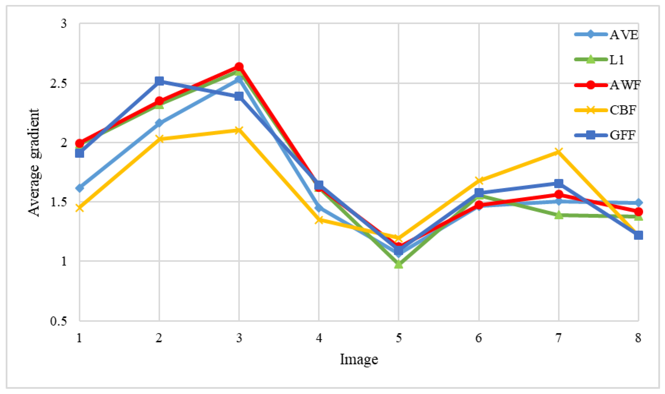
Image	Average Gradient of Results (Percentage Change)
	AVE	L1	AWF	CBF	GFF
Figure 13a	1.618	1.985 (22.7%)	1.995 (23.3%)	1.452 (−10.3%)	1.91 (18.0%)
Figure 13b	2.163	2.321 (7.3%)	2.349 (8.6%)	2.029 (−6.2%)	2.514 (16.2%)
Figure 13c	2.533	2.6 (2.6%)	2.639 (4.2%)	2.103 (−17.0%)	2.386 (−5.8%)
Figure 13d	1.451	1.621 (11.7%)	1.624 (11.9%)	1.347 (−7.2%)	1.642 (13.2%)
Figure 13e	1.063	0.975 (−8.3%)	1.121 (5.5%)	1.195 (12.4%)	1.092 (2.7%)
Figure 13f	1.462	1.556 (6.4%)	1.474 (0.8%)	1.679 (14.8%)	1.576 (7.8%)
Figure 13g	1.505	1.389 (−7.7%)	1.564 (3.9%)	1.92 (27.6%)	1.656 (10.0%)
Figure 13h	1.491	1.377 (−7.6%)	1.42 (−4.8%)	1.217 (−18.4%)	1.222 (−18.0%)
Average	-	- (3.4%)	- (6.7%)	- (−0.5%)	- (5.5%)

show the average gradient of the output images in different sea surface scenarios with different methods. Table A1 provides the quantitative image quality assessment of eight groups of fused images.

According to the results in Figure 13 and Table A1, the AWF algorithm had a stable effect, and its overall average gradient improved by 6.7% compared to the AVE method. Other indicators also performed well. The CBF algorithm had a clear gap with the other methods in most indicators. The performance of the GFF method varied greatly in different scenarios. It performed slightly worse than the AWF method in terms of the average gradient index and showed a 5.5% improvement compared to the AVE method.

In conclusion, according to the qualitative and quantitative image quality assessment, the AWF fusion strategy is more suitable than other fusion strategies for sea images.

5. Conclusions

In this paper, three fusion strategies were proposed to combine with neural networks to improve the quality of water surface images in response to the image degradation problem existing in the marine environment. First, calibration of the infrared and visible cameras equipped on the USV was carried out using a self-designed calibration board to estimate the camera parameters. Then, visible and infrared images of the USV’s operating environment were aligned, utilizing these parameters. Finally, the pairs of aligned images were used as the input for the network to verify the superiority of the proposed methods.

The quality of images generated by the proposed methods was evaluated according to a variety of indicators. Compared to AVE, the average image fusion gradient based on the AWF increased by 6.7%. The CBF had no obvious advantage over the original algorithm (AVE and L1). The GFF performed better than other methods, but there was a color distortion problem in the images. The proposed AWF showed superior performance to other methods, in most cases, in two aspects of the qualitative and quantitative image quality assessment that was carried out.

The experiments showed that, compared to the existing methods AVE and L1 from [28], AWF is more suitable for water surface scenes and can be applied in USV visual systems. It can improve the image quality to help USVs better identify targets and complete various complex tasks.

References

- Liu, Z.; Zhang, Y.; Yu, X.; Yuan, C. Unmanned surface vehicles: An overview of developments and challenges. Annu. Rev. Control. 2016, 41, 71–93. [Google Scholar] [CrossRef]
- Huang, B.; Zhou, B.; Zhang, S.; Zhu, C. Adaptive prescribed performance tracking control for underactuated autonomous underwater vehicles with input quantization. Ocean. Eng. 2021, 221, 108549. [Google Scholar] [CrossRef]
- Campbell, S.; Naeem, W.; Irwin, G.; Campbell, S.; Naeem, W.; Irwin, G. A review on improving the autonomy of unmanned surface vehicles through intelligent collision avoidance manoeuvres. Annu. Rev. Control. 2012, 36, 267–283. [Google Scholar] [CrossRef] [Green Version]
- Ma, Z.; Wen, J.; Zhang, C.; Liu, Q.; Yan, D. An effective fusion defogging approach for single sea fog image. Neurocomputing 2016, 173, 1257–1267. [Google Scholar] [CrossRef]
- Ma, J.; Ma, Y.; Li, C. Infrared and visible image fusion methods and applications: A survey. Inf. Fusion 2019, 45, 153–178. [Google Scholar] [CrossRef]
- Singh, R.; Vatsa, M.; Noore, A. Integrated multilevel image fusion and match score fusion of visible and infrared face images for robust face recognition. Pattern Recognit. 2008, 41, 880–893. [Google Scholar] [CrossRef] [Green Version]
- Zhu, C.; Zeng, J.; Huang, B.; Su, Y.; Su, Z. Saturated approximation-free prescribed performance trajectory tracking control for autonomous marine surface vehicle. Ocean. Eng. 2021, 237, 109602. [Google Scholar] [CrossRef]
- Zhou, B.; Huang, B.; Su, Y.; Zheng, Y.; Zheng, S. Fixed-time neural network trajectory tracking control for underactuated surface vessels. Ocean. Eng. 2021, 236, 109416. [Google Scholar] [CrossRef]
- Kumar, P.; Mittal, A.; Kumar, P. Fusion of Thermal Infrared and Visible Spectrum Video for Robust Surveillance. In Computer Vision, Graphics and Image Processing; Springer: Berlin/Heidelberg, Germany, 2006; pp. 528–539. [Google Scholar]
- Simone, G.; Farina, A.; Morabito, F.C.; Serpico, S.B.; Bruzzone, L. Image fusion techniques for remote sensing ap-plications. Inf. Fusion 2002, 3, 3–15. [Google Scholar] [CrossRef] [Green Version]
- Ma, Z.; Wen, J.; Liang, X. Video Image Clarity Algorithm Research of USV Visual System under the Sea Fog. In Proceedings of the International Conference in Swarm Intelligence, Harbin, China, 12–15 June 2013; Springer Science and Business Media LLC: Berlin/Heidelberg, Germany, 2013; Volume 7929, pp. 436–444. [Google Scholar]
- Zabolotskikh, E.V.; Mitnik, L.; Chapron, B. New approach for severe marine weather study using satellite passive microwave sensing. Geophys. Res. Lett. 2013, 40, 3347–3350. [Google Scholar]
- Zhu, C.; Huang, B.; Zhou, B.; Su, Y.; Zhang, E. Adaptive model-parameter-free fault-tolerant trajectory tracking control for autonomous underwater vehicles. ISA Trans. 2021, 114, 57–71. [Google Scholar] [CrossRef] [PubMed]
- Zhang, H.; Wang, X.; Luo, X.; Xie, S.; Zhu, S. Unmanned surface vehicle adaptive decision model for changing weather. Int. J. Comput. Sci. Eng. 2021, 24, 18–26. [Google Scholar] [CrossRef]
- Liu, Y.; Jin, J.; Wang, Q.; Shen, Y.; Dong, X. Region level based multi-focus image fusion using quaternion wavelet and normalized cut. Signal. Process. 2014, 97, 9–30. [Google Scholar] [CrossRef]
- Toet, A. Image fusion by a ratio of low-pass pyramid. Pattern Recognit. Lett. 1989, 9, 245–253. [Google Scholar] [CrossRef]
- Choi, M.; Kim, R.Y.; Nam, M.-R.; Kim, H.O. Fusion of Multispectral and Panchromatic Satellite Images Using the Curvelet Transform. IEEE Geosci. Remote Sens. Lett. 2005, 2, 136–140. [Google Scholar] [CrossRef]
- Wang, J.; Peng, J.; Feng, X.; He, G.; Fan, J. Fusion method for infrared and visible images by using non-negative sparse representation. Infrared Phys. Technol. 2014, 67, 477–489. [Google Scholar] [CrossRef]
- Li, S.; Yin, H.; Fang, L. Group-sparse representation with dictionary learning for medical image denoising and fusion. IEEE Trans. Biomed. Eng. 2012, 59, 3450–3459. [Google Scholar] [CrossRef]
- Wang, Z.; Cui, Z.; Zhu, Y. Multi-modal medical image fusion by Laplacian pyramid and adaptive sparse representation. Comput. Biol. Med. 2020, 123, 103823. [Google Scholar] [CrossRef]
- Zhu, Z.; Yin, H.; Chai, Y.; Li, Y.; Qi, G. A novel multi-modality image fusion method based on image decomposition and sparse representation. Inf. Sci. 2018, 432, 516–529. [Google Scholar] [CrossRef]
- Xing, C.; Wang, M.; Dong, C.; Duan, C.; Wang, Z. Using Taylor Expansion and Convolutional Sparse Representation for Image Fusion. Neurocomputing 2020, 402, 437–455. [Google Scholar] [CrossRef]
- Wu, C.; Chen, L. Infrared and visible image fusion method of dual NSCT and PCNN. PLoS ONE 2020, 15, e0239535. [Google Scholar] [CrossRef] [PubMed]
- Zhong, Z.; Gao, W.; Khattak, A.M.; Wang, M. A novel multi-source image fusion method for pig-body multi-feature detection in NSCT domain. Multimed. Tools Appl. 2020, 79, 26225–26244. [Google Scholar] [CrossRef]
- Li, H.; Wu, X.-J. Multi-focus Image Fusion Using Dictionary Learning and Low-Rank Representation. In Proceedings of the International Conference on Image and Graphics, Shanghai, China, 13–15 September 2017; Springer Science and Business Media LLC: Berlin/Heidelberg, Germany, 2017; pp. 675–686. [Google Scholar]
- Liu, Y.; Chen, X.; Peng, H.; Wang, Z. Multi-focus image fusion with a deep convolutional neural network. Inf. Fusion 2017, 36, 191–207. [Google Scholar] [CrossRef]
- Liu, Y.; Chen, X.; Ward, R.K.; Wang, Z.J. Image Fusion With Convolutional Sparse Representation. IEEE Signal. Process. Lett. 2016, 23, 1882–1886. [Google Scholar] [CrossRef]
- Li, H.; Wu, X.-J. DenseFuse: A Fusion Approach to Infrared and Visible Images. IEEE Trans. Image Process. 2019, 28, 2614–2623. [Google Scholar] [CrossRef] [PubMed] [Green Version]
- Ram Prabhakar, K.; Sai Srikar, V.; Venkatesh Babu, R. Deepfuse: A deep unsupervised approach for exposure fusion with extreme exposure image pairs. In Proceedings of the IEEE International Conference on Computer Vision, Venice, Italy, 22–29 October 2017; pp. 4714–4722. [Google Scholar]
- An, G.H.; Lee, S.; Seo, M.-W.; Yun, K.; Cheong, W.-S.; Kang, S.-J. Charuco Board-Based Omnidirectional Camera Calibration Method. Electronics 2018, 7, 421. [Google Scholar] [CrossRef] [Green Version]
- Ch, M.M.I.; Riaz, M.M.; Iltaf, N.; Ghafoor, A.; Ahmad, A. Weighted image fusion using cross bilateral filter and non-subsampled contourlet transform. Multidimens. Syst. Signal. Process. 2019, 30, 2199–2210. [Google Scholar] [CrossRef]
- Hayat, N.; Imran, M. Ghost-free multi exposure image fusion technique using dense SIFT descriptor and guided filter. J. Vis. Commun. Image Represent. 2019, 62, 295–308. [Google Scholar] [CrossRef]