Numerical Simulation of Cavitation Flow in a Low Specific-Speed Centrifugal Pump with Different Diameters of Balance Holes

Abstract

In order to study the influence of a balance hole’s diameter on the cavitation performance of low specific-speed centrifugal pumps, a centrifugal pump with a specific speed of 0.301 was selected as the research object. The pump’s cavitation performance, distribution of cavitation vapor in the impeller, and axial force on the impeller were studied with the change in diameters of balance holes. The results show that with the increase in the diameter of balance holes, the cavitation number σ_3% of the low specific-speed centrifugal pump became small, the pressure in the mechanical seal cavity dropped gradually, and the flow velocity in balance holes was reduced. As cavitation occurred in the impeller, the diameter of balance holes not only affected the absolute value of the axial force but also affected the direction of the axial force.

1. Introduction

Centrifugal pumps are widely used in industrial and agricultural irrigation fields in daily life, and are also key equipment in the fields of aviation, naval, and other extremely technical fields [1,2,3]. When a centrifugal pump operates at high speed, the axial force is exerted on the rotor due to the asymmetry of the front and rear cover plates of the impeller, and a large axial force can affect the normal operation of the pump. In order to balance the axial force, balance holes accompanied with a sealing ring are usually adopted during designing [4].

However, due to the existence of the mentioned balance holes, high-pressure fluid can flow into the inlet of the centrifugal impeller from balance holes and change the flow state at the impeller inlet, and the scheme of balance holes has a certain impact on the performance of a centrifugal pump [5]. So far, domestic and foreign scholars have conducted much research on the influence of balance holes on the internal flow characteristics of centrifugal pumps. Sha [6] studied the influence of balance holes on the performance of high-temperature and high-pressure centrifugal pumps, and pointed out that if the size and distribution of balance holes are appropriate, the axial force can be effectively balanced, that the performance of centrifugal pumps is comparable to those of centrifugal pumps without balance holes, and that the axial force can effectively be reduced by about 15%. The leakage rate of the liquid in the hub cavity of the centrifugal pump was calculated and compared with the test result by Dong [7], and according to the research, when no balance hole existed, the distribution of liquid velocity in the core area of the hub cavity exhibited axial symmetry and the circumferential velocity component was approximately 0.4 times of the impeller’s rotation speed, whereas when the balance hole existed, the distribution of liquid velocity in the hub cavity did not exhibit axial symmetry and the circumferential velocity component was larger than 0.4 times of the impeller’s rotational speed. González [8] studied the capability of a numerical simulation in capturing the dynamic and unsteady flow effects inside a centrifugal pump due to the impeller-volute interaction. Time-averaged numerical results were compared with the experimental performance curve and good agreement was found, and the amplitude of the fluctuating pressure field at the blade-passing frequency was successfully captured by the model for a wide range of operating flow rates. Fathi [9] found that a centrifugal pump increasing balancing hole diameters up to 5 mm could lead to a 5.6% reduction in head at design flow rate. Furthermore, it was also found that the diameter of the balancing hole affected the pump efficiency and could reduce it by 2.6%, and numerical investigation showed that the diameter of the balancing hole could play a prominent role in reducing the axial force significantly. Extreme care must be taken in selecting the diameter of balancing holes since increasing the hole diameter beyond a specific value does not reduce the axial force significantly, but still aggravates the pump performance undesirably. Barrio [10] estimated the dynamic radial force and torque at the blade-passing frequency as a function of flow rate and blade-tongue radial gap. They estimated that for a given impeller diameter, the dynamic load would increase for off-design conditions, especially for the low range of flow rates, whereas the progressive reduction in the impeller-tongue gap would bring about corresponding increments in dynamic load; in particular, varying the blade-tongue gap within the limits resulted in multiplying the maximum magnitude of the blade-passing frequency radial force by a factor of about four for low flow rates and three for high flow rates. Ding [11] provided a novel CFD methodology and an advanced cavitation model with which key components relevant to the improvement of accuracy and CFD simulation speed were discussed in detail, and an axial flow water pump was chosen as the test case to demonstrate and validate the capability and accuracy of the code discussed. Simulation results included pump head, hydraulic efficiency, and cavitation characteristics in terms of the incipient net positive suction head for the whole pump flow passages using both multiple reference frames and transient approaches. Multiple operation conditions from 70% to 120% of the design flow rate were evaluated and projected against experimental data. Roohi [12] and Pendar [13] used OpenFOAM software to simulate the cavitation flow and super cavitation flow behind the three-dimensional disk, compared the differences between turbulence models and cavitation models in detail, and analyzed the flow characteristics under different cavitation numbers. Tran [14] analyzed the adaptability of Kubota and Merkle cavitation models to NACA66 hydrofoil cavitation flow and the difference in the cavitation cloud evolution law. The hydraulic cavitation performance and pressure pulsation characteristics of the pump were obtained under different operating conditions based on steady and transient numerical simulations of the flow field in a centrifugal pump [15], and the pressure pulsation amplitude reduced with cavitation development, and the dominant frequency of the pulsation was the blade-passing frequency. With extending cavitation degrees, the high-frequency components in the pressure pulsation became rich, and the dominant frequency at each monitoring point dropped significantly. Ye [16] used machine learning methods to monitor the running status of a centrifugal pump and to make judgments on the initial cavitation status before cavitation failures occurred in the centrifugal pumps, so as to provide a research foundation for online monitoring technology of centrifugal pumps.

Existing studies have mainly focused on the influence of balance holes on the internal flow characteristics and the axial force on common centrifugal pumps, while studies on the effect of balance holes on cavitation flow characteristics of low specific-speed centrifugal pumps are lacking. Based on the Zwart-Gerber-Belamri (ZGB) cavitation model [17], a centrifugal pump with a specific speed of 0.301 was selected as the research object, and CFX software was adopted to simulate the inner full flow domain of the pump. The cavitation characteristics of the low specific-speed centrifugal pump with different diameters of balance holes were studied. The purpose of this paper was to completely study the influence of changes in the diameter size of balance holes of the low specific-speed centrifugal pump on cavitation occurring, and also show the cavitation flow in the pump as well as the axial force characteristics on the impeller.

2. Research Object and Meshing

2.1. Research Object

The research object was the ACB13-24 low specific-speed centrifugal pump, of which the design flow rate Q = 13 m³/h, design head H = 24 m, the rotation speed n = 2880 r/min, and the specific speed $n_s=\varpi \sqrt{Q/3600}/{(gH)}^{0.75}=2\pi n\sqrt{Q/3600}/60{(gH)}^{0.75}=0.301$. The pump’s structural assembly drawing is shown in Figure 1. The pump was of low-noise, and it was designed and manufactured by the authors. The pump was mainly used for clean water transportation. This pump’s main components included volute, impeller, seal ring, mechanical sealing, motor, etc. Impeller inlet diameter D₁ = 44 mm, impeller outlet diameter D₂ = 146 mm, blade outlet width b₂=6mm, blade number N = 5, volute base circle diameter D₃ = 150 mm, the diameter of the seal ring D_m = 51.7 mm, and the gap size of the seal ring δ = 0.3 mm.

2.2. Balance Hole Sketch

The axial force on the impeller of the low specific-speed centrifugal pump was balanced by using a sealing ring and balance holes on the impeller, as shown in Figure 2. The flow channel between each blade in the impeller had a balance hole with its different size. The balance of the axial force mainly depended on the gap size of the seal ring, the diameter of the seal ring, and the total area of balance holes. In order to facilitate the description of the diameter of balance holes, the ratio of total area of balance holes to the gap area of the seal ring is defined in Equation (1). In this paper, besides the original pump model, three other models with different diameters of balance holes were proposed to facilitate the study on the relationship between the diameter of the balance hole and the cavitation characteristics of the low specific-speed centrifugal pump. The geometric parameters of balance holes are shown in

Table 1. Geometric parameters of balance holes.

Program	$\mathit{\xi }$	Φ (mm)
Original model	1.5	3
model 1	1	2
model 2	3	4.3
model 3	4	5

.

$$\xi =\frac{N\frac{1}{4}\pi {\varphi }^2}{\frac{1}{4}\pi \left({\left(D_{\mathrm{m}}+2\delta \right)}^2-D_{\mathrm{m}}^2\right)}\approx \frac{N{\varphi }^2}{4\delta D_{\mathrm{m}}}$$

(1)

The number of balance holes N was 5, ϕ is the diameter of balance holes, D_m was the diameter of the seal ring, and δ was the gap size of the seal ring. Since δ in the Equation (1) was much smaller than D_m, square of δ was omitted from the final expression.

2.3. Computational Domain and Meshing

Figure 3 shows the three-dimensional computational domain of the low specific-speed centrifugal pump modeled by three-dimensional modeling software Creo 4.0, and the computational domain mainly included the extension section, inlet, front cavity, volute, impeller, rear cavity, and mechanical seal cavity. Balance holes combined with the impeller belonged to the same rotation domain. In order to describe exactly the direction of axial force, a three-dimensional coordinate system was also given in Figure 3, where the positive direction of the z-axis was from the rear cavity to the inlet.

The meshing software ICEM 15.0 was used to mesh the computational domain with a hexahedral structure. During the process of meshing, the number of nodes were changed and controlled; key parts such as the impeller blade surfaces and vicinity of volute tongue were locally encrypted to meet the y+ requirements of 30~200 for the modified RNG k-ε turbulence model. The blocks in the impeller flow channel and the blocks in balance holes were transitioned by the O-shaped meshing method. In the end, the number of impeller grids with four different diameters of balance holes was all controlled at about 810,000, the number of volute grids was controlled at about 484,000, and total number of grids was about 2.1 million. The grid distributions of the volute and impeller are shown in Figure 4, and average y+ on flow parts from simulation results was about 60.

Five sets of grids with different numbers were designed for grid independence inspection, the design flow rate of 13 m³/h was chosen for numerical simulation, and heads of the pump with five sets of grids were obtained. Values of grids and heads are listed in

Table 2. Grid independence verification.

	Grid 1	Grid 2	Grid 3	Grid 4	Grid 5
Impeller grid number	55,060	99,416	472,440	809,230	1,114,004
Hole grid number	1814	3226	12,158	24,460	30,224
Volute grid number	34,360	53,576	320,702	484,106	594,454
Total grid number	500,143	816,030	1,597,421	2,079,601	2,412,153
Head (m)	26.6423	26.3295	25.7424	25.5283	25.5186
Power (kW)	1.4782	1.403	1.3682	1.3546	1.352
Efficiency (%)	63.81	66.44	66.61	66.72	66.82

, and with the increase in the number of grids, the head (H), power (P), and efficiency ($\eta$) tended to be stable. Considering the factors of accuracy and time cost, scheme of grid 4 was selected for subsequent simulation, and the number of grids in balance holes was 24,460. Power (P) was obtained from simulation, $P=M\varpi /1000$, unit, kW, where M is the torque on the impeller, N·m and $\varpi$ is the angular velocity, 1/s. Efficiency ($\eta$) was defined as, $\eta =\rho gQH/3600/1000P$, where $\rho$ is the density, 1000 kg/m³, g is the gravitational acceleration, 9.81 m²/s , Q is flow rate, m³/h, and H is head, m. Uncertainty of H, P, and $\eta$ obtained from simulation results with grid 3, grid 4, and grid 5 were analyzed as follows.

$\overline{X}$ is the average of simulation results, $\overline{X}={\displaystyle \sum _{i=1}^3{x}_i}/3$, where $x_i$ is the simulation result with grid 3, grid 4, or grid 5. Standard deviation (SD) was calculated by $SD=\sqrt{{\displaystyle \sum _{i=1}^3(x_i-\overline{X}}{)}^2/2}$. Uncertainty (U) was calculated by $U=SD/\sqrt{3}\overline{X}$. Uncertainty of H, P, and $\eta$ obtained from simulation results with grid 3, grid 4, and grid 5 was 0.4%, 0.37%, and 0.091%, respectively.

3. Numerical Simulation Method

3.1. Governing Equation

Cavitation flow could be regarded as an ideal homogeneous flow, the mixed flow model was used to establish two-phase flow model, and the control equations of this homogeneous equilibrium flow could be expressed as follows:

$$\frac{\partial {\rho }_{\mathrm{m}}}{\partial t}+\frac{\partial ({\rho }_{\mathrm{m}}{u}_{\mathrm{j}})}{\partial x_{\mathrm{j}}}=0$$

(2)

$$\frac{\partial {\rho }_{\mathrm{m}}{u}_{\mathrm{i}}}{\partial t}+\frac{\partial \left({\rho }_{\mathrm{m}}{u}_{\mathrm{i}}{u}_{\mathrm{j}}\right)}{\partial x_{\mathrm{j}}}=-\frac{\partial p}{\partial x_{\mathrm{i}}}+\frac{\partial }{\partial x_{\mathrm{j}}}\left[\left(\mu +{\mu }_{\mathrm{t}}\right)\left(\frac{\partial u_{\mathrm{i}}}{\partial x_{\mathrm{j}}}+\frac{\partial u_{\mathrm{j}}}{\partial x_{\mathrm{i}}}-\frac{2}{3}\frac{\partial u_{\mathrm{i}}}{\partial x_{\mathrm{j}}}{\delta }_{\mathrm{ij}}\right)\right]$$

(3)

In above formula, ρ_m is the density of the mixed medium, t is the time, the subscripts i and j are the coordinate directions, u_i and u_j are the velocity components, μ and μ_t are the dynamic viscosity and turbulent viscosity of the mixed medium, respectively, and δ_ij is Kronecker inner product.

3.2. Turbulence Model and Cavitation Model

The filter turbulence model proposed by Johansen et al. [18] was chosen and used to modify the RNG k-ε model (FBM RNG). This turbulence model combines the advantages of the Reynolds time-average method and the LES (large-eddy simulation) method. Compared with the ordinary LES method, coarser grid in the boundary layer is allowed. The turbulent viscosity was modified in this method, and expressions of the k equation and ε equation remained unchanged. The modified expressions are as follows:

$${\mu }_{\mathrm{t}}=\frac{{\rho }_{\mathrm{m}}{C}_{\mathsf{\mu }}{k}^2}{\epsilon }F,\hspace{1em}{C}_{\mathsf{\mu }}=0.09$$

(4)

In the formula, F is the filter function, and its size is determined by the filter size λ and the turbulence length scale k^3/2/ε. The relationship is expressed as follows:

$$F=min[1,C_3\frac{\lambda \epsilon }{k^{3/2}}],\hspace{1em}{C}_3=1$$

(5)

In order to ensure that filtering process can be achieved, the filter size λ should not be less than the grid size ∆ of the simulation area. ∆x, ∆y, and ∆z represent the grid length of the water domain in three coordinate directions in the impeller, ∆ = (∆x∆y∆z)^1/3. According to the above formula written in CFX, the RNG k-ε model based on filtering correction was obtained by compiling the CFX expression language (CEL).

The cavitation model is a mathematical model that describes the mutual transformation between vapor and liquid in the flow field. When cavitation occurs in the flow field, a phase change process occurs between the gas phase and liquid phase, and the inter-phase transmission expression is as follows:

$$R=R_{\mathrm{e}}-R_{\mathrm{c}}$$

(6)

In order to describe the process of cavitation development and collapse accurately, the ZGB cavitation model was adopted which is the default mass transfer model in CFX software. The model was derived from the basic equations of Rayleigh–Plesset [19] cavitation dynamics:

$$R_{\mathrm{e}}=F_{\mathrm{vap}}\frac{3{\alpha }_{\mathrm{ruc}}\left(1-{\alpha }_{\mathrm{v}}\right){\rho }_{\mathrm{v}}}{R_{\mathrm{B}}}\sqrt{\frac{2}{3}\frac{P_{\mathrm{v}}-P}{{\rho }_{\mathrm{l}}}};\hspace{1em}P<P_{\mathrm{v}}$$

(7)

$$R_{\mathrm{c}}=F_{\mathrm{cond}}\frac{3{\alpha }_{\mathrm{v}}{\rho }_{\mathrm{v}}}{R_{\mathrm{B}}}\sqrt{\frac{2}{3}\frac{P-P_{\mathrm{v}}}{{\rho }_{\mathrm{l}}}};\hspace{1em}P>P_{\mathrm{v}}$$

(8)

In the formula, α_ruc is the volume fraction at the nucleation site, and the value is 5 × 10⁻⁴; ρ_v is the vapor phase density; α_v is the vapor phase volume fraction; R_B is the cavity radius, 1 × 10⁻⁶ m; P and P_v are the flow field pressure and vaporization pressure, respectively, and the unit is Pa; and F_vap and F_cond are the empirical coefficients of vapor generation and condensation process, set to 50 and 0.01, respectively. Usually, the condensation process is much slower than the evaporation process, so F_cond is much smaller than F_vap.

3.3. Boundary Conditions and Solution Control

The computational domain grid was imported into the simulation software CFX19.0 for pre-processing settings. The entire flow field was set to a three-dimensional incompressible steady viscous turbulent flow, the turbulence model was set to the FBM RNG model, and the inlet and outlet boundary conditions were set to total pressure inlet and mass flow rate outlet, respectively. The entire computational domain was divided into a rotating and stationary domain. The impeller domain belonged to the rotating domain and its rotation speed was set to be 2880 r/min, and other computational domains were set to be the stationary domain. A frozen rotor was used at the interface between the rotating domain and the stationary domain, and the wall surface roughness of each part was set to 0.025 mm according to manufacture accuracy. The simulation setting of the cavitation flow was slightly different from that of the non-cavitation flow. The liquid phase and cavitation vapor phase were created in the material. According to the water temperature in the experiment, the properties of the two phases were set to the physical parameters at 17 °C, as shown in

Table 3. Physical parameters of water and vapor at 17 °C.

Property Parameter	Water	Vapor
Saturated vapor pressure (Pa)	1938	1938
Density (kg/m3)	998.73	0.0145
Specific heat capacity (kJ/kg·K)	4.187	1.902
Specific enthalpy (kJ/kg)	71.36	2532
Specific entropy (kJ·kg·K)	0.253	8.734
Thermal expansion coefficient (10−4·K)	2.57	33.6

. The homogeneous multiphase flow model was set in the fluid domain where the turbulence model remained unchanged. The saturated vapor pressure during cavitation was set to be 1938 Pa, and the average vapor bubble diameter was set to be 1 × 10⁻⁶ mm. There was no relative slip between phases, no heat transfer, and no consideration of surface tension. The initial volume fraction of the vapor phase was set to be 0, and the volume fraction of the liquid phase was set to be 1. In the solution control, the SIMPLEC algorithm was used, the second-order upwind discrete difference equation was adopted, the maximum iteration step was set to 1000, and the convergence accuracy was 10⁻⁴.

3.4. Experiment Verification

3.4.1. External Characteristic Experiment

In order to verify the accuracy of the simulation results, the ACB13-24 low specific-speed centrifugal pump was experimented for external characteristics on an open test bench, as shown in Figure 5. The flow rate was controlled by adjusting the inlet control valve and outlet control valve.

3.4.2. Experimental Results

Figure 6 shows the experimental performance curves of the pump, where Q_T denotes the flow rate, m³/h, H_T denotes the head, m, P_T denotes the shaft power, kW, ${\eta }_T$ denotes efficiency, %, ${\eta }_T=\rho g{Q}_T{H}_T/3600/1000P_T$, and BEP denotes the flow rate at the best efficiency point. It can be seen that the head gradually decreased with the increase in the flow rate; under the design flow rate of 13 m³/h, the experimental head was 24.28 m, which was close to the design value. It can also be seen from the efficiency curve that as the flow rate increased, the efficiency first rose then fell, and BEP slightly deviated from the design flow rate. When the flow rate was 14.34 m³/h, the highest efficiency reached 65.61% where the head was 23.28 m.

3.4.3. Comparison of Simulation with Experimental Results

In order to verify the accuracy of the simulation results, the pump’s head and efficiency performance curves obtained from experiment and simulation results were plotted in the same coordinate system for comparative analysis, as shown in Figure 7a. It can be seen that the head and efficiency from the simulation were close to those from experimental results, and the change trends were also similar. The head gradually decreased and the efficiency first rose then decreased with the increase in flow rate. Although there were certain gaps between experiment results and simulation results, gaps were within allowable range of error; therefore, the simulation results were considered to be credible.

The following dimensionless parameters were defined, and head coefficient ψ and cavitation number σ were expressed as follows:

$$\psi =H/\left(u_2^2/2g\right)$$

(9)

$$\sigma =\left(P_{\mathrm{in}}-P_{\mathrm{v}}\right)/0.5\rho u_2^2$$

(10)

where, u₂ is the circumferential velocity at the impeller outlet, m/s; H is the pump head, m; g is the gravity acceleration, 9.81 m/s²; and P_in and P_v are pump inlet pressure and saturated vapor pressure, respectively, p_a.

As shown in Figure 7b, at a flow rate of 13 m³/h, the simulation results were consistent with the experimental results in terms of variation trends, and the phenomenon of the pump head coefficient dropping suddenly after the cavitation number decreased to the inflection point could be predicted.

4. Simulation Results Analysis

4.1. Influence of Diameter of Balance Holes on External Characteristics

Figure 8 shows the cavitation performance of the centrifugal pump under different ξ. The cavitation number σ_3% when the head dropped by 3% was still used as the criterion for cavitation performance of the low specific-speed centrifugal pump; that is to say, σ_3% was the cavitation number when cavitation occurred. It can be seen that the simulation cavitation results under different ξ showed a consistent trend. When the cavitation number σ was large, cavitation had not occurred, and the head remained unchanged with the change in the cavitation number, but the head decreased with the increase in the diameter of balance holes. The head coefficient under ξ = 4 was about two percent less than that under ξ = 1. There were two main reasons for this phenomenon: first, from the perspective of energy loss, not all high-pressure fluid at the outlet of the impeller flowed into the volute; a part of the high-pressure fluid leaked through the rear cavity into the balance holes and flowed back to the inlet of the impeller, and fluid leaking caused direct energy loss, then the head dropped; second, the fluid leaking to the inlet of the impeller impacted the main flow in the impeller and destroyed the normal flow streamline, resulting in an extra drop of the pump’s head.

As the cavitation number decreased, the head coefficient began to show an inflection point. As shown in Figure 8, as $\xi$ became larger, σ_3% gradually decreased, which indicated that cavitation in the low specific-speed centrifugal pump did not easily occur with the increase in the diameter of balance holes. When the diameter of balance holes became larger, the leakage area of balance holes also became larger; under the condition that other parameters remained unchanged, leakage flow velocity in balance holes as well as leakage flow velocity at the impeller inlet dropped. The main impact due to the existence of balance holes was weak, so there was no obvious effect on the cavitation performance of the pump. When the diameter of balance holes was small, the velocity of leakage flow in the balance holes was higher, and the impact and damage to the main flow in the impeller were greater. It may be easy to form a local low-pressure zone at the inlet of the impeller, and a local low-pressure zone can accelerate the cavitation process in the centrifugal pump.

4.2. Influence of Balance Hole Diameter on Cavitation Internal Flow Characteristics

4.2.1. The Influence of Balance Hole Diameter on Flow Velocity and Pressure

Figure 9 shows the velocity distribution in the low specific-speed centrifugal pump with different diameters of balance holes under cavitation number σ_3% at the axial section. After fluid in the centrifugal pump impeller flowed out of the impeller, a part of the fluid leaked into the rear cavity, and then returned to the impeller inlet through balance holes. When $\xi$ = 3 and $\xi$ = 4, the leakage flow in balance holes did not fuse with the main flow in the impeller uniformly, and there was a tendency to generate vortices at the junction of balance holes and the impeller flow channel, but the velocity of the leakage flow was low, and impacts of leakage flow on the mainstream was weak. When $\xi$ = 1, flow was relatively smooth in balance holes, and it directly merged with main flow in the impeller after flowing out of balance holes; however, because the flow velocity was high, it was easy to cause a local low-pressure zone at the inlet of the impeller and lead to cavitation. When $\xi$ = 1.5, compared with those of $\xi$ = 3 and $\xi$ = 4, the flow in balance holes was more stable, no low-speed zone formed, leakage velocity from balance holes was almost the same as the flow velocity in the impeller, and the convergence with the mainstream was smooth. When $\xi$ = 1, excessively high velocity distribution in balance holes inevitably impacted or damaged the mainstream.

Figure 10 shows the pressure distribution in the pump with different diameters of balance holes under cavitation number σ_3% at the axial section. It can be seen that the pressure distribution of the flow field of each model had obvious stratification. Because of the existence of cavitation, a large area of low pressure existed at the inlet of the impeller. With the increase of $\xi$, the pressure in the mechanical seal cavity dropped. This was related to the operation characteristics of the balance hole, the main function of balance holes being to relieve pressure in the mechanical seal cavity and to balance the axial force. Therefore, when the diameter of balance holes became larger, the pressure in the mechanical seal cavity of course dropped.

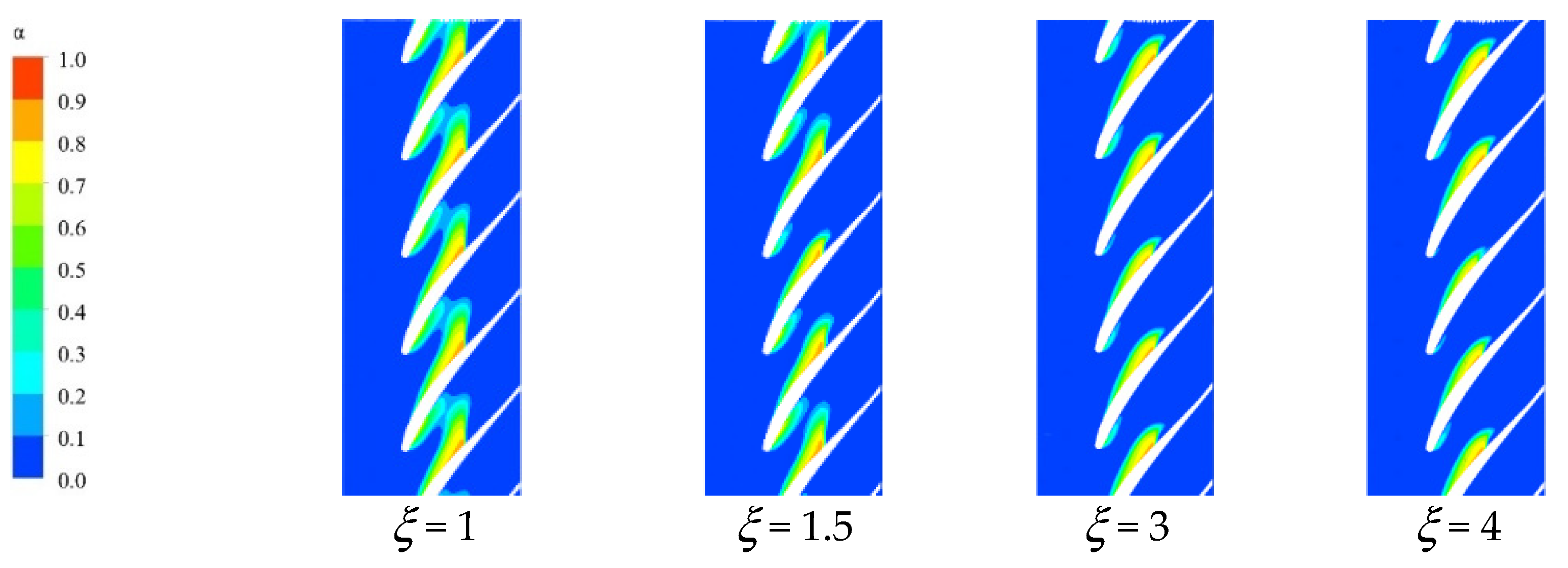
4.2.2. Cavitation Vapor Distribution in Impeller with Different Diameters of Balance Holes

The hub surface is displayed in black and was defined as span = 0, the rim surface is displayed in green and was defined as span = 1, as shown in Figure 11a, and span = 0.8 is the yellow turbo surface, as shown in Figure 11b. Because the surface of span = 0.8 was located at the position where the centrifugal pump impeller blades were prone to cavitation occurring, the surface of span = 0.8 was selected to show the blade-to-blade plot here.

Figure 12 shows the volume fraction distribution of the cavitation vapor with different ξ at the surface of span = 0.8. In the impeller, under σ = 0.038, the cavitation vapor distribution in the impeller under different balance hole diameters was quite different, and cavitation vapor appeared on the pressure and suction sides of blades in all four models. If ξ ≥ 3, although cavitation vapor on the pressure and suction sides of blades had formed, it was only confined to the front edges of blade inlets. When ξ was small, especially when ξ = 1, cavitation vapor on the pressure sides extended and almost connected to cavitation vapor on the suction sides.

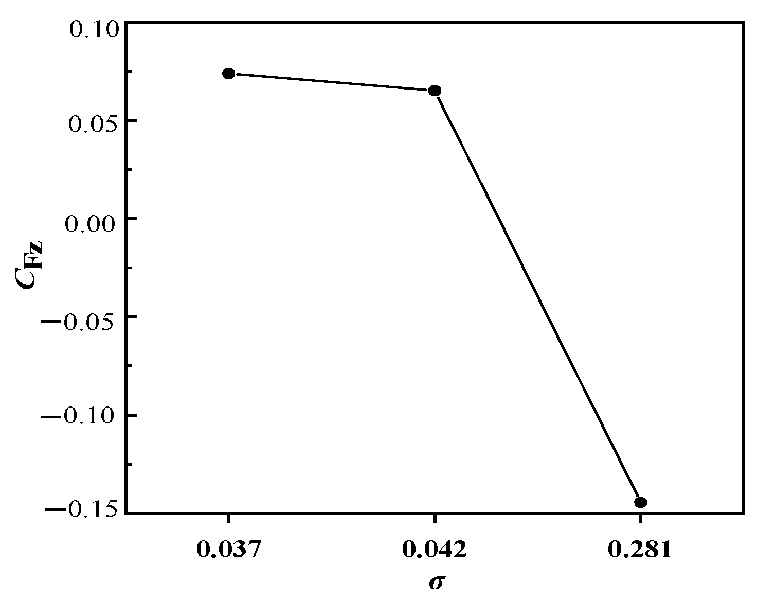
4.3. Influence of Balance Hole Diameter and Cavitation on Axial Force

Figure 13 shows the distribution of the axial force on the impeller at different flow rates, $\xi$ = 1.5, without cavitation. A positive or negative value in the figure only indicates the direction. The axial force coefficient was defined as:

$$C_{\mathrm{Fz}}=\frac{2F_z}{\rho u_2^2{D}_2{b}_2}$$

(11)

where, F_z is the absolute value of the axial force on the impeller, N; ρ is density, kg/m³; u₂ is the circumferential velocity at the impeller outlet, m/s; and b₂ is the blade outlet width of the impeller, m.

The axial force on the impeller increased with the increase in flow rate, and the direction of the force was in the negative direction of the z-axis (from the impeller inlet to the rear cover), which was mainly related to the impact of the pressure on the impeller. The greater the flow rate was, the greater the absolute value of the axial force on the impeller was.

Figure 14 shows the distribution of the axial force on the impeller under different cavitation numbers at a design flow rate, $\xi$ = 1.5. When the cavitation number σ was 0.281, cavitation had not occurred in the impeller, and the axial force was still in the negative direction of the z-axis. As the cavitation number decreased, a low-pressure zone began to appear in the impeller. When σ = 0.042, the axial force decreased and changed its direction (from the impeller rear cover to the impeller inlet). Cavitation happened, then the pressure distributions of the flow domain including the front and rear cavities altered. In addition, it was easy to form cavitation near balance holes and even block balance holes; furthermore, pressure relief from balance holes was reduced. At this time, the pressure in the mechanical seal cavity was greater than the pressure at the inlet in the impeller, so the axial force changed to the positive direction of the z-axis. When σ = 0.037, cavitation occurred in the pump, and the blockage was serious in the impeller and balance holes. The pressure in the mechanical seal cavity was still greater than that at the inlet in the impeller, the axial force increased slightly, but the direction had not changed.

Figure 15 shows the distribution of the axial force on the impeller with different diameters of balance holes under σ_3%. It can be seen that, due to the difference in the diameter of balance holes, the axial force on the impeller also showed a huge difference. When $\xi$ = 1, the axial force was the largest in the positive direction of the z-axis. Because the diameter of balance holes was the smallest, the pressure in the mechanical seal cavity did not sufficiently relieve from balance holes, and as cavitation occurred in the pump, the mechanical seal cavity was filled with a large number of cavitation vapors which further blocked balance holes. Then the fluid in the mechanical seal cavity could not leak completely, the pressure in the mechanical seal cavity was high, and the axial force acting on the rear cover plate of the impeller was significantly greater than that acting on front cover plate of the impeller, and as a result, the axial force was the largest in the positive direction of the z-axis. When $\xi$ = 1.5, the diameter of balance holes became large, and the axial force was also in the positive direction of the z-axis. When $\xi$ ≥ 3 , the axial force on the impeller turned in the negative direction of the z-axis. As the balance hole diameter increased to $\xi$ = 4, the absolute value of the axial force increased slightly.

5. Conclusions

The influence of the balance hole diameter on the cavitation performance, vapor distribution, and axial force on the impeller of the low specific-speed centrifugal pump was studied. The main conclusions were as follows:

(1) Without cavitation, as the diameter of balance holes increased, the pump’s head gradually decreased. In addition, as $\xi$ increased, σ_3% gradually decreased.

(2) Under σ_3%, when $\xi$ = 1, flow in balance holes was relatively smooth; however, it was easy to cause a local low-pressure zone at the inlet of the impeller channel. When $\xi$ = 1.5, compared with those of $\xi$ = 3 and $\xi$ = 4, the flow in balance holes was more stable, and leakage velocity from balance holes was almost the same as the velocity at the inlet in the impeller; as a result, the convergence with the mainstream was weak.

(3) Without cavitation, the axial force on the impeller increased with the increase in the flow rate, and the axial force was in the positive direction of the z-axis. The diameter of balance holes not only affected the absolute value of the axial force but also affected the direction of the axial force. Under σ_3%, when $\xi$ = 1, the axial force was in the positive direction of the z-axis and decreased as $\xi$ increased, and when $\xi$ ≥ 3, the axial force was in the negative direction of the z-axis and its absolute value increased slightly.

References

1. Guam, X. Theory and Design of Modern Pump; China Aerospace Press: Beijing, China, 2011. [Google Scholar]
2. Zhao, W.; Wang, D.; Liu, Z. Optimal design of low-to-medium specific speed centrifugal pump based on genetic algorithm. J. Lanzhou Univ. Technol. 2017, 43, 56–59. [Google Scholar]
3. Yuan, S. Theory and Design of Low Specific Speed Centrifugal Pump; China Machine Press: Beijing, China, 1996. [Google Scholar]
4. Liu, Z.; Lu, W.; Zhao, W.; Chen, T. Effect of balance holes and back blades on axial thrust of centrifugal pump. J. Drain. Irrig. Mach. 2019, 37, 834–840. [Google Scholar]
5. Liu, Z.; Yang, K.; Lu, W.; Su, D. Influence of balance hole diameter on flow pattern of centrifugal pump impeller inlet. J. Drain. Irrig. Mach. Eng. 2020, 38, 973–978. [Google Scholar]
6. Sha, Y.; Liu, S.; Wu, Y.; Wang, B. Study on the influence of balance holes on the performance of high temperature and high pressure centrifugal pumps. J. Hydroelectr. Eng. 2012, 31, 259–264. [Google Scholar]
7. Dong, W.; Chu, W.L.; Liu, Z.L. Influence of the diameter of the balance hole on the flow characteristics in the hub cavity of the centrifugal pump. J. Hydrodyn. 2019, 31, 1060–1068. [Google Scholar] [CrossRef]
8. González, J.; Fernández, J.; Blanco, E.; Santolaria, C. Numerical simulation of the dynamic effects due to impeller-volute interaction in a centrifugal pump. ASME J. Fluids Eng. 2002, 124, 348–355. [Google Scholar] [CrossRef]
9. Fathi, M.; Raisee, M.; Nourbakhsh, S.A.; Arani, H.A. The effect of balancing holes on performance of a centrifugal pump: Numerical and experimental investigations. IOP Conf. Ser. Earth Environ. Sci. 2019, 240, 032017. [Google Scholar] [CrossRef]
10. Barrio, R.; Blanco, E.; Parrondo, J.; González, J.; Fernández, J. The effect of impeller cutback on the fluid-dynamic pulsations and load at the blade-passing frequency in a centrifugal pump. ASME J. Fluids Eng. 2018, 130, 111102. [Google Scholar] [CrossRef]
11. Ding, H.; Visser, F.C.; Jiang, Y.; Furmanczyk, M. Demostration and validation of a 3D CFD simulation tool predicting pump performance and cavitation for industrial applications. ASME J. Fluids Eng. 2011, 133, 011101. [Google Scholar] [CrossRef]
12. Roohi, E.; Pendar, M.R.; Rahimi, A. Simulation of three-dimensional cavitation behind a disk using various turbulence and mass transfer models. Appl. Math. Model. 2016, 40, 542–564. [Google Scholar] [CrossRef]
13. Pendar, M.R.; Roohi, E. Investigation of cavitation around 3D hemispherical head-form body and conical cavitators using different turbulence and cavitation models. Ocean. Eng. 2016, 112, 287–306. [Google Scholar] [CrossRef]
14. Tran, T.D.; Nennemann, B.; Vu, T.C. Investigation of cavitation models for steady and unsteady cavitating flow simulation. Int. J. Fluid Mach. Syst. 2015, 8, 240–253. [Google Scholar] [CrossRef]
15. Wang, K.; Li, H.; Shen, Z. Pressure pulsation characteristics in down-scaled high specific speed centrifugal pump in cavitating state. J. Drain. Irrig. Mach. Eng. 2020, 38, 891–897. [Google Scholar]
16. Ye, T.; Si, Q.; Shen, C.; Yang, S.; Yuan, S. Monitoring of primary cavitation of centrifugal pump based on support vector machine. J. Drain. Irrig. Mach. Eng. 2021, 39, 884–889. [Google Scholar]
17. Zwart, P.J.; Gerber, A.G.; Belamri, T. A two-phase flow model for predicting cavitation dynamics. In Proceedings of the ICMF 2004 International Conference on Multiphase Flow, Yokohama, Japan, 30 May–3 June 2004; pp. 1–11. [Google Scholar]
18. Johansen, S.T.; Wu, J.; Shyy, W. Filter-based unsteady rans computations. Int. J. Heat Fluid Flow 2004, 25, 10–21. [Google Scholar] [CrossRef]
19. Zhang, D.; Zhang, Q.; Shi, W. Numerical Simulation Basis and Application of Vane Pump Design; China Machine Press: Beijing, China, 2015. [Google Scholar]
Figure 1. Structural assembly drawing.
Jmse 10 00619 g001
Figure 2. Balance hole sketch.
Jmse 10 00619 g002
Figure 3. Computational domain.
Jmse 10 00619 g003
Figure 4. Grid of volute and impeller. (a) volute; (b) impeller.
Jmse 10 00619 g004
Figure 5. Centrifugal pump opening test bench. (a) Schematic diagram of the pump experiment; (b) test site; and (c) data collection.
Jmse 10 00619 g005
Figure 6. Experimental performance curves of the pump.
Jmse 10 00619 g006
Figure 7. Comparison of simulation with experiment. (a) head and efficiency results comparison; (b) cavitation results comparison.
Jmse 10 00619 g007
Figure 8. Curve of head with σ and ξ .
Jmse 10 00619 g008
Figure 9. Velocity distribution at axial section under σ3%.
Jmse 10 00619 g009
Figure 10. Pressure distribution at axial section under σ3%.
Jmse 10 00619 g010
Figure 11. Surfaces at different spans. (a) hub and rim surface; (b) surface of span = 0.8.
Jmse 10 00619 g011
Figure 12. Vapor volume fraction in impeller with different ξ.
Jmse 10 00619 g012
Figure 13. Distribution of axial force on the impeller at different flow rates.
Jmse 10 00619 g013
Figure 14. Distribution of axial force on the impeller under different cavitation numbers.
Jmse 10 00619 g014
Figure 15. Distribution of axial force on the impeller with different ξ under σ3%.
Jmse 10 00619 g015