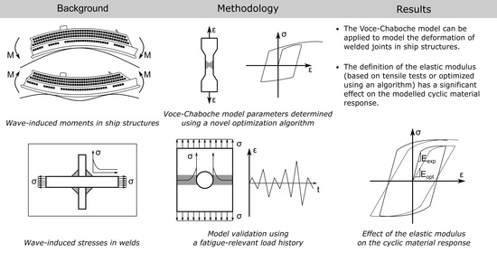
Optimizing the Voce–Chaboche Model Parameters for Fatigue Life Estimation of Welded Joints in High-Strength Marine Structures

Abstract

This work studies the Voce–Chaboche (V–C) material model parameter optimization for high-strength steel welded joints subjected to cyclic loading. The model parameters of each material zone in a S690 steel butt-welded joint were determined using an optimization algorithm based on the Newton trust region (NTR) method and an accumulated true strain parameter. The model parameters were fitted to stress–strain histories from uniaxial strain-controlled cyclic tests. To validate the model, fully-reversed variable amplitude fatigue experiments were performed under load control. The experimental results were then compared to numerical results from a finite element analysis. When the elastic modulus is optimized as a V–C parameter, the results indicate that the V–C model slightly underestimates the strain range, leading to conservative fatigue life estimates. However, the results can be improved by using an elastic modulus obtained experimentally. In this case, the resulting material model slightly overestimates the strain range, leading to a non-conservative, but more accurate, fatigue life estimation. It can be concluded that the NTR-based accumulated true strain approach successfully determined the V–C model parameters for different material zones in the welded joint, and closely estimated the strain range and the fatigue life for a variable amplitude load history.

1. Introduction

In many civil applications, welded joints introduce geometric discontinuities and material nonlinearities [1]. This is particularly relevant in ship structures, as a cruise ship has around 1000 km of welded joints [2]. Welds are often located at structural discontinuities, such as connections of structural elements, and they can include notches and undercuts acting as stress raisers [3,4,5]. Additionally, the local microstructure surrounding a weld is altered during the welding process, leading to material nonlinearities. For high-performing welds, this material effect is as damaging as any geometrical effect [6]. Improvements in manufacturing technologies have led to a decrease in the size of defects present in welded joints. Due to these developments, the most relevant fatigue failure process changed from macro-crack propagation (defect size of about $0.1$ mm) towards fatigue crack initiation [6]. This paradigm shift allows the utilization of high-strength steels and higher loads, leading to larger material plasticity around stress concentrations. However, current design guidelines for welded joints assume only linear elastic material behavior [7]. Consequently, the recommended fatigue life assessment methods are unable to accurately estimate the fatigue life of high-performing welded joints in lightweight ship structures [8]. One of the existing challenges is modeling the material plasticity and stress–strain behavior of the weld, which can change under cyclic loads [9], e.g., loads caused by wave–ship interaction. Improved fatigue life estimation methods for high-performing welded joints need to consider both the elastic and plastic material response, including transient material effects, such as isotropic and kinematic hardening [8].

Transient material effects can be considered by the Voce–Chaboche (V–C) cyclic plasticity model. Among its applications, it has been used to study the cyclic behavior of welded steel joints subjected to low cycle fatigue [10,11,12], and the redistribution of residual stresses during elastic shakedown [13] or after high-frequency mechanical impact (HFMI) treatment [14]. Finally, the V–C model has also been used to study the effect of seismic loading on steel structures such as moment-resisting frames [15,16], buckling-restrain braces [17], or pressure-retaining metal components in nuclear power plants [18]. One shortcoming of the V–C model is the lack of a universally accepted model parameters optimization algorithm [19]. In the original paper, Chaboche et al. [20] determined the model parameters for 316 stainless steel through manual curve-fitting of different expressions to five stabilized cyclic hysteresis loops. However he acknowledged that “automatic identification procedures could be used”. Nonetheless, many researchers still choose to determine the V–C model parameters using manual curve-fitting methods applied to stabilized hysteresis loops [21,22,23] or to cyclic stress–strain curves [24]. This process is often reduced to an inefficient trial-and-error approach [25,26]. Other popular methods of determining the V–C model parameters use genetic algorithms [19,27,28] or particle swarm optimization (PSO) [25].

Recently, de Castro e Sousa et al. [15] developed a new model parameter estimation approach. This process uses a Newton trust region (NTR) method to minimize an error function that is defined by the true stress and the accumulated true strain. This formulation of the inverse problem presents a more robust alternative to genetic algorithms and particle swarm optimization methods [15]. The optimization procedure is implemented in a Python library named RESSPyLab (Resilient Steel Structures Laboratory Python Library) [29]. The proposed methodology consists of three phases: application-relevant load protocol sampling, material and testing procedures, and parameters determination. This methodology has successfully determined the V–C model parameters of several different types of structural steel [15], and of the base material and the HAZ of welded S690 QL high-strength steel [11] under low cycle fatigue.

This paper focuses on the experimental validation of the V–C material model applied to high-strength steel welded joints subjected to cyclic loading. The aim is to apply the V–C material model to estimate strains of different material zones of welded joints subjected to fatigue-relevant loads. This study uses the NTR-based accumulated true strain approach [15] to optimize the V–C model parameters for the base metal (BM), the heat-affected zone (HAZ), and the weld metal (WM). The considered cyclic loads are representative of the fatigue-relevant loads acting on a cruciform welded joint located in an upper deck longitudinal deck girder of a large cruise ship. To the best of the authors’ knowledge, no other studies have used the V–C model to represent the cyclic material behavior limited to the transition region between elastic and plastic material behavior. Neither has the NTR-based accumulated true strain been applied to determine V–C model parameters to describe the material response around the yield stress of a material. Therefore, the parameter optimization methodology outlined in [15] is modified to provide the best results for the material behavior expected in welded joints in ship structures. The fitness of the resulting V–C model is determined by comparing numerical results from a finite element analysis to experimental results. The evaluation criteria focus on the strain range per load cycle, as this is a relevant quantity for fatigue life estimation using a strain–life approach.

The structure of the paper is as follows: Section 2 introduces the V–C cyclic plasticity model and the chosen model parameter estimation method. Section 3 presents the methodology for the V–C model parameter estimation and the finite element analysis (FEA). Section 4 presents the results of the material model parameter estimation experiments and the validation experiments. Section 5 presents the discussion. The main findings of the paper are summarized in Section 6, the conclusion.

2. Theoretical Background

This section presents the theoretical framework for the uniaxial V–C model in the J2 plasticity framework. First, the general equations of the V–C model are introduced. Second, the material model parameter optimization method developed by de Castro e Sousa et al. [15] is summarized briefly.

2.1. Uniaxial Voce–Chaboche Model

The V–C model is a nonlinear isotropic and kinematic hardening model that combines the Voce isotropic hardening law [30] and the Chaboche kinematic hardening law [20]. In the Haigh–Westergaard stress space, the isotropic hardening law describes how the yield surface (defined by the von Mises criterion) expands or contracts as a function of the equivalent plastic strain ${\epsilon }_{eq}^p$,

$${\sigma }_y={\sigma }_{y0}+Q_{\infty }\left(1-e^{-b{\epsilon }_{eq}^p}\right),$$

(1)

where ${\sigma }_{y0}$ is the initial yield stress of the material, $Q_{\infty }$ is the maximum saturated value by which the yield stress can change, and b is the exponential saturation parameter that describes the rate of change of the yield stress.

The kinematic hardening law describes how the origin of the yield surface shifts in the stress space as a function of the equivalent plastic strain rate ${\dot{\epsilon }}_{eq}^p$. This shift is called the backstress $\alpha$. In the Chaboche hardening law, the total backstress $\alpha$ is calculated as the sum of the individual backstresses ${\alpha }_i$. Each backstress ${\alpha }_i$ is described by an Armstrong–Franklin rule [31],

$${\dot{\alpha }}_i=\mathrm{sign}\left(\sigma -\alpha \right)C_i{\dot{\epsilon }}_{eq}^p-{\gamma }_i{\alpha }_i{\dot{\epsilon }}_{eq}^p,$$

(2)

where $C_i$ is the $ith$ kinematic stress parameter and $\gamma$ is the $ith$ kinematic saturation parameter. The total backstress is calculated as

$$\alpha =\sum _{i=1}^N{\alpha }_i,\mathrm{i}=1,2,\dots ,\mathrm{N},$$

(3)

where N is the total number of backstresses. In the uniaxial load case, the equivalent plastic strain rate ${\dot{\epsilon }}_{eq}^p$ can be calculated as

$${\dot{\epsilon }}_{eq}^p=\left|{\dot{\epsilon }}^p\right|.$$

(4)

2.2. Accumulated True Strain Approach and RESSPyLab

The methodology proposed by de Castro e Sousa et al. [15] uses service-relevant stress–strain histories to determine the V–C model parameters for a specific material. In their original work, the proposed strain-based load protocols were representative of the deformation in steel moment-resisting frames subjected to seismic loads. Tensile test coupons were subjected to these load protocols in order to collect the applied load signal F and the corresponding controlled strain signal ${\epsilon }_{\mathrm{eng}}$. These signals were then converted to true stress and true strain using the well-known relations

$$\begin{array}{cc}\hfill {\epsilon }_{\mathrm{true}}& =ln(1+{\epsilon }_{\mathrm{eng}}),\mathrm{and}\hfill \end{array}$$

(5)

$$\begin{array}{cc}\hfill {\sigma }_{\mathrm{true}}& =\frac{F}{A_0}(1+{\epsilon }_{\mathrm{eng}}),\hfill \end{array}$$

(6)

where $A_0$ is the initial cross-sectional area of the test coupon. In the case of cyclic loading, a stress value ${\sigma }_{\mathrm{true}}$ can be attributed to multiple strain values ${\epsilon }_{\mathrm{true}}$ due to cycling-induced changes in the mechanical properties of the material. To link each stress value to an unique strain value, the accumulated true strain parameter ${\epsilon }^{*}$ was introduced.

$${\epsilon }^{*}={\int }_0^t\left|{\dot{\epsilon }}_{\mathrm{true}}\right|\mathrm{d}\tau .$$

(7)

Consequently, the true stress ${\sigma }_{\mathrm{true}}$ can be expressed as a function of the accumulated true strain ${\epsilon }^{*}$. The goal of the material parameter optimization routine is to find the best-fitting stress signal ${\sigma }_{\mathrm{model}}$ for an input accumulated true strain signal ${\epsilon }^{*}$. The error function that is to be minimized during the parameter estimation process is

$$\phi ({\epsilon }^{*};\mathsf{\theta })=\sum _i\frac{{\int }_0^{{\epsilon }^{*}}{\left[{\sigma }_{\mathrm{model}}\left({\epsilon }_i^{*};\mathsf{\theta }\right)-{\sigma }_{\mathrm{Test}}\right]}^2\mathrm{d}{\epsilon }^{*}}{{\int }_0^{{\epsilon }^{*}}\mathrm{d}{\epsilon }^{*}},i\in \left\{1,\dots ,n_{\mathrm{Test}}\right\},$$

(8)

where $n_{\mathrm{Test}}$ is the number of considered input signals. The vector $\mathsf{\theta }$ contains all of the parameters that need to be determined during the parameter estimation process, namely,

$$\mathsf{\theta }=\left\{\mathrm{E},{\sigma }_{y0},Q_{\infty },b,C_1,{\gamma }_1,\dots ,C_i,{\gamma }_i\right\}$$

(9)

Each component of the vector $\mathsf{\theta }$ is restricted within ${\mathsf{\theta }}_i\le 1\times {10}^{-4}$. The error function $\phi ({\epsilon }^{*};\mathsf{\theta })$ is minimized using the NTR approach. For more information on the optimization procedure, see [15].

3. Materials and Methods

This section presents the methodology for each experiment performed as a part of this study: (a) V–C model parameter estimation, (b) experimental V–C model validation, and (c) numerical V–C model validation using a finite element analysis. Since the material parameter estimation experiments and the model validation experiments follow similar methodologies, they are presented together in Section 3.1 and Section 3.2. Section 3.3 is dedicated to the finite element analysis.

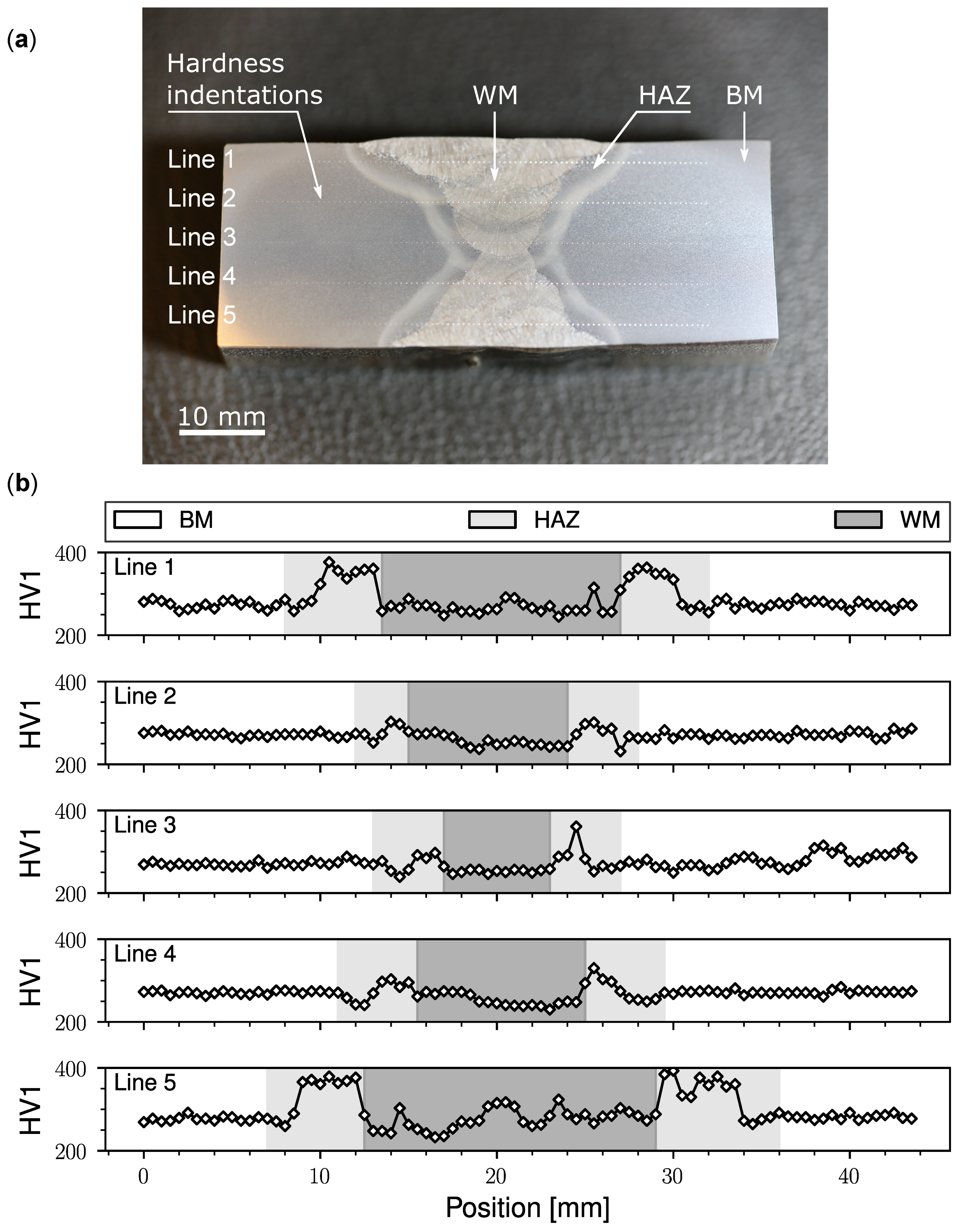
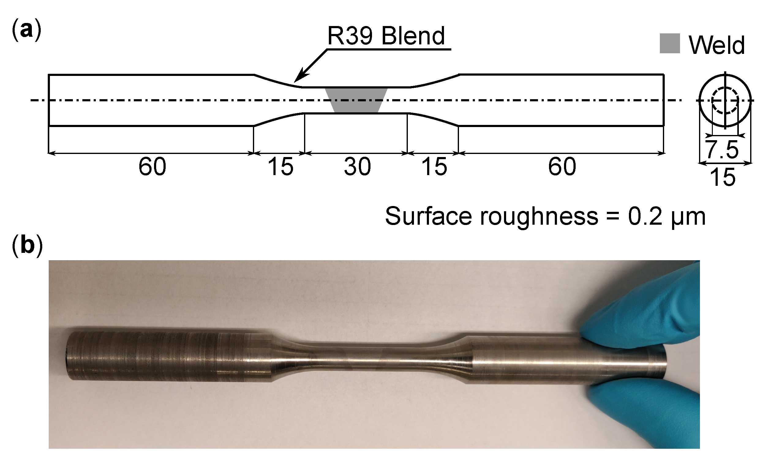
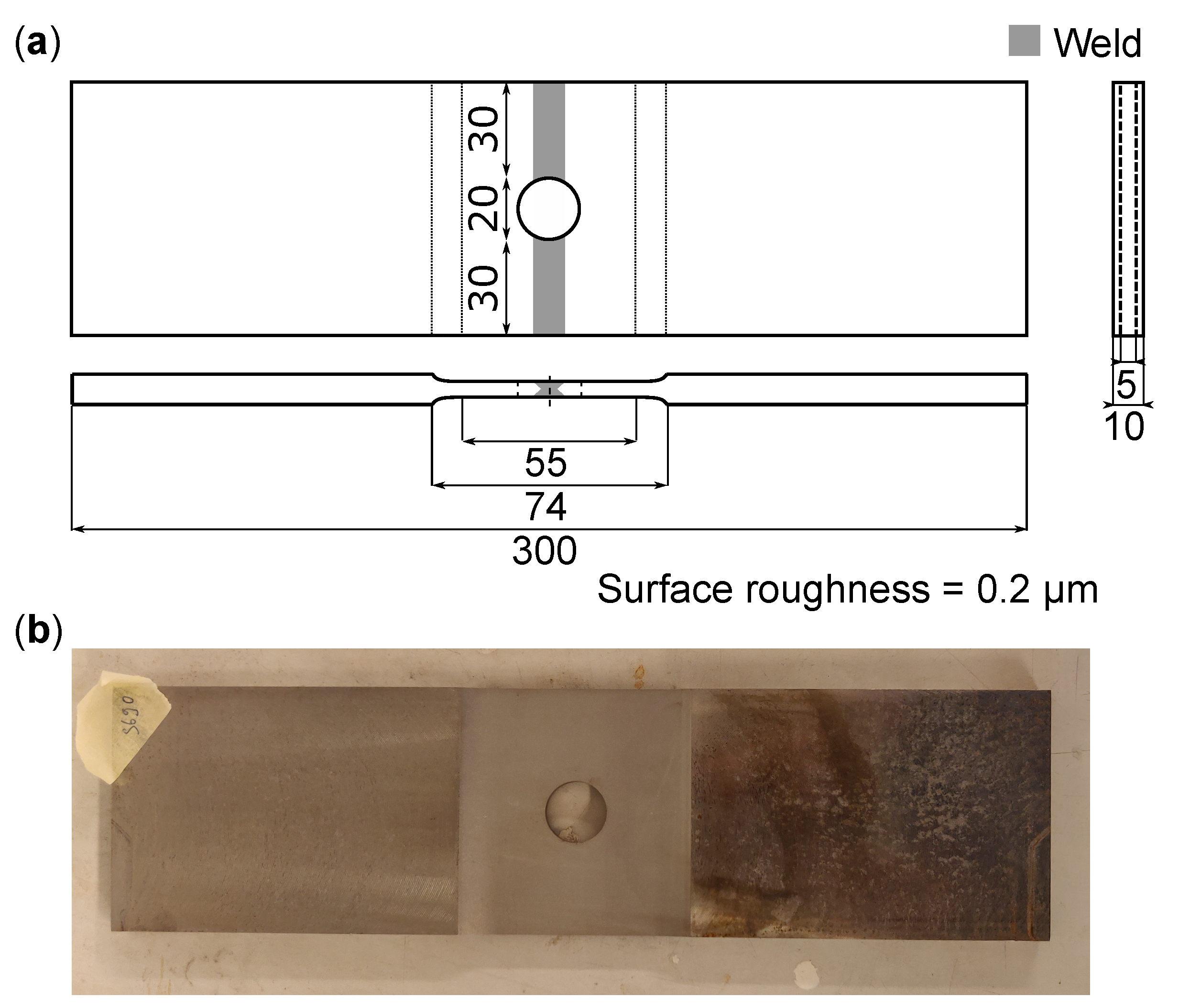
3.1. Material and Weld Samples

The test specimens were manufactured from butt-welded S690 steel plates provided by the shipyard Meyer Turku Oy. Figure 1 shows a macro sample of the weld and the corresponding hardness profile. The base material consists of two 22 mm thick plates made of S690 SHIP QT from SSAB. The base material has a reported yield stress of 854 MPa, an ultimate tensile stress of 874 MPa, and an area reduction of 16%. The butt-welds were generated from an X-groove through metal active gas (MAG) welding. The filler material was OUTERSHIELD 690-H $1.2$ mm. Its reported as-welded mechanical properties are a yield stress of 780 MPa, an ultimate tensile stress of 810 MPa, and an area reduction of 18%. The chemical composition of both materials is presented in

Table 1. Chemical composition of S690 Ship QT in mass percent % as specified by the manufacturer.

C	Si	Mn	P	S	Al	Nb	V	Ti	Cu	Cr	Ni	Mo	N	B	CET
$0.159$	$0.19$	$1.42$	$0.007$	$0.002$	$0.036$	$0.016$	$0.021$	$0.009$	$0.012$	$0.25$	$0.04$	$0.498$	$0.003$	$0.0013$	$0.36$

and

Table 2. Chemical composition of Outershield 690-H in maximum mass percent % (except for C) as specified by the manufacturer.

C	Si	Mn	P	S	Cr	Ni	Mo	Cu	V	Ti	Al	As	Sn	Pb	N
$0.805$	$0.01$	$0.01$	$0.001$	$0.001$	$0.01$	$0.01$	$0.01$	$0.01$	$0.01$	$0.001$	$0.001$	$0.001$	$0.001$	$0.001$	$0.001$

. The quality of the weld was assessed through radiography and ultrasonic inspection.

Hardness tests were performed using a Struers Duramin-40 tabletop hardness testing machine. Hardness measurements were taken with a load of 1 kgf and a Vicker’s hardness indenter. The optical resolution was set according to ISO standards [32]. The Vicker’s hardness (HV) results were converted to the Brinell hardness (HB) scale as proposed by [33]. The average Brinell hardness was used to estimate the coefficients of the Coffin–Manson–Basquin strain–life relationship according to [34].

The standard deviation ${\sigma }_{\mathrm{SD}}$ of the hardness measurements is provided. The average hardness values at the center of the macro sample were 271 HV1 (257 HB) in the base material (${\sigma }_{\mathrm{SD}}=6$ HV1) and in the HAZ (${\sigma }_{\mathrm{SD}}=12$ HV1), and 254 HV1 (241 HB) in the weld material (${\sigma }_{\mathrm{SD}}=14$ HV1).

Figure 2 and Figure 3 present the geometries of the test specimens manufactured from the welded plates and used in the material parameter estimation experiments and the validation experiments. The material parameter estimation experiments were performed using round dog-bone specimens designed according to ASTM standards [35]. The validation experiments were performed on plates with a circular hole at the center of the test section. The circular hole is placed in the weld to introduce a stress concentration effect comparable to that of a micro notch at the weld toe of a cruciform-welded joint [36]. The specimen design was validated against buckling through finite element analysis. To manufacture the dog-bone specimens, the original welded plate was cut into individual strips. Each strip was machined into a test specimen using CNC machining. To manufacture the flat specimens, wider sections of the original welded plates were cut. These plates were then milled to the outer dimensions of the specimen. The test section and the circular notch were realized using electrical discharge machining (EDM). Both types of test specimens had a surface roughness of 0.2 µm in the test section.

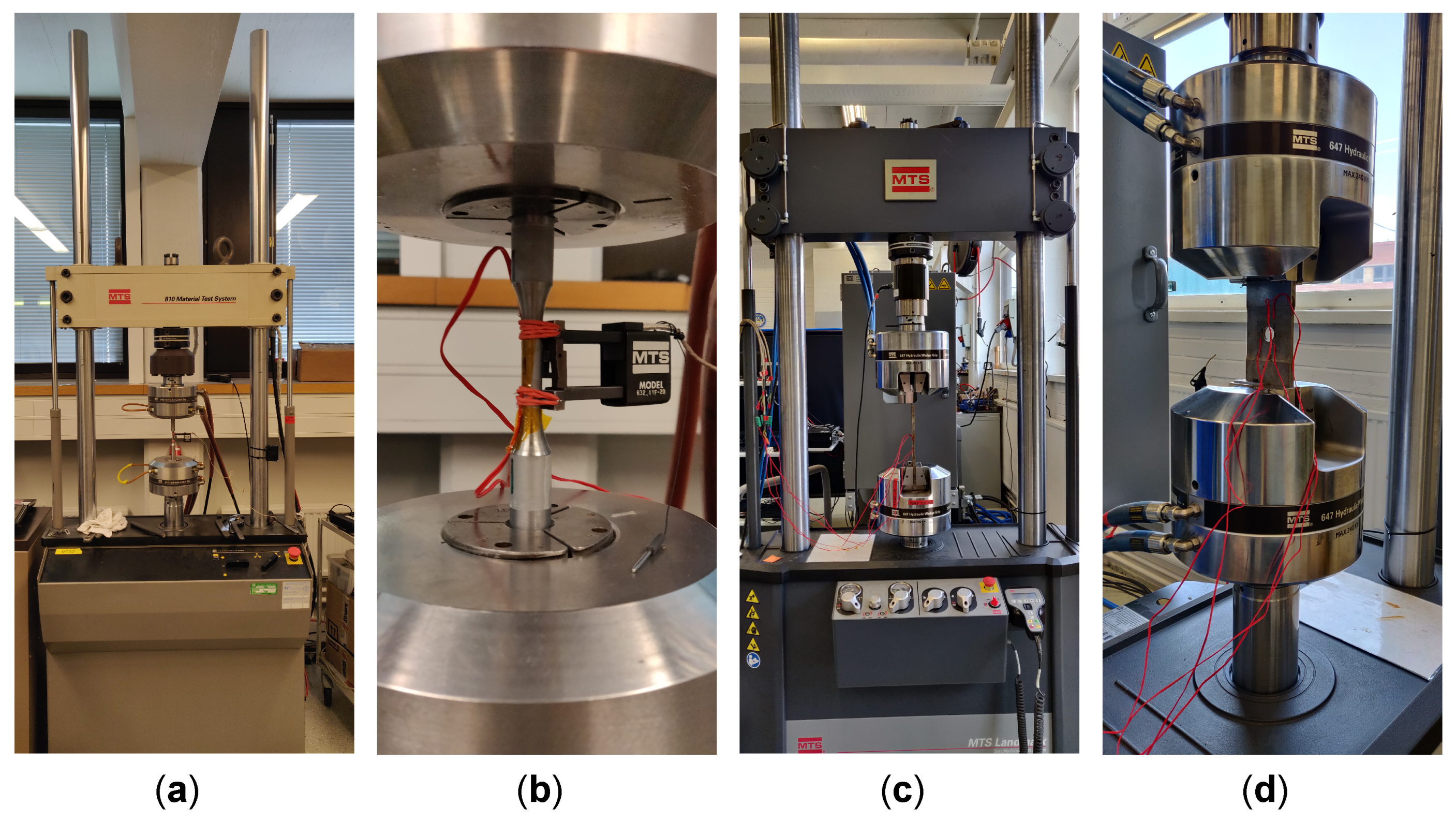
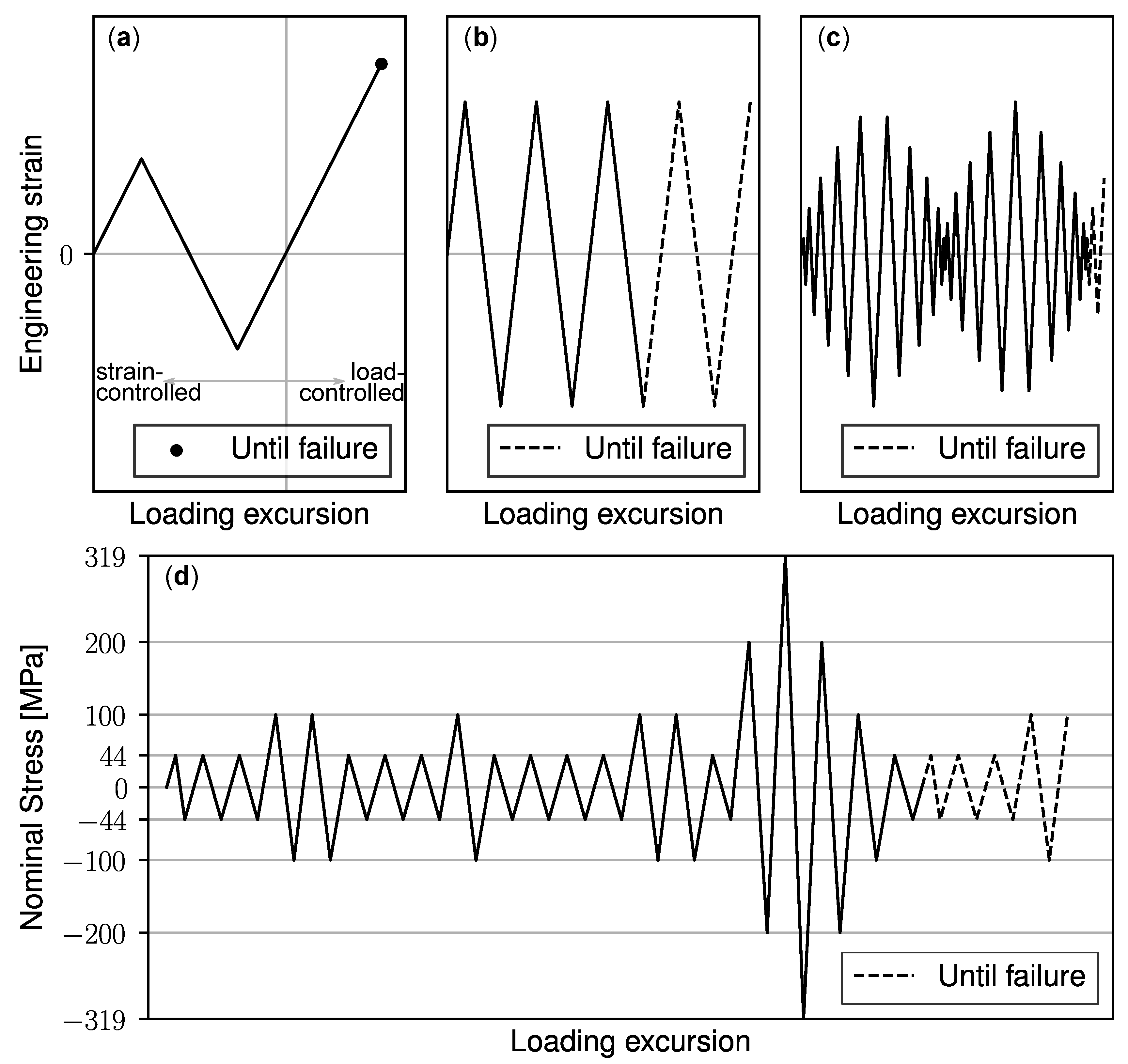
3.2. Experimental Test Setup

Two different experimental test setups were used for the material parameter estimation experiments and the validation experiments. The strain-controlled material parameter estimation experiments were performed using the MTS-810 servo-hydraulic test system in combination with an MTS Model 632.11F-20 extensometer with a gauge length of 25 mm. The dog-bone test specimens were held in place using the 646 Hydraulic Collet Grip. The load-controlled validation experiments were performed using the MTS 370.50 servo-hydraulic test system with a load capacity of 250 kN. The flat specimens were held in place using wedge grips of type 647 Hydraulic Wedge Grips with smooth clamping wedges. An L-shaped guide was used to align the flat specimens. Each experimental test setup is presented in Figure 4.

The load protocols used in the material parameter estimation experiments and the validation experiments considered the recommendations by [15] and fatigue-relevant load cycles as proposed in the DNV standard [37]. In the present study, three different load protocols were used: (a) one fully-reversed load cycle and tension until failure, (b) fully-reversed constant amplitude cyclic loading, and (c) an incremental step test (see Figure 5). The latter two protocols are standard material characterization tests [38]. The controlled strain range was chosen to be representative of the expected service loads and to guarantee stable structural behavior. The validation load protocol consisted of a load block with 21 fully-reversed, variable amplitude load cycles (see Figure 5d). The load block is representative of fatigue-relevant stresses experienced in high-performing welds in large cruise ship structures. The reader is referred to [36] for additional information on the choice of load amplitudes. Each load protocol was repeated until one of the strain gauges failed. Here, failure is defined as measuring a strain that exceeded the measurement range of 5%.

Table 3. Overview of the material parameter estimation experiments and the validation experiments. Each load protocol is fully reversed. The strain amplitude ${\epsilon }_a$ is given in percent %.

Load Protocol	Specimen [#]	${\mathit{\epsilon }}_{\mathit{a}}$ [%]	Analyzed Signal
One cycle and tension	2	$1.0$	Whole signal
One cycle and tension	1	$2.0$	Whole signal
Constant amplitude	5	$0.5$	First five cycles
Constant amplitude	6	$0.5$	First five cycles
Constant amplitude	3	$1.0$	First five cycles
Constant amplitude	4	$1.0$	First five cycles
Incremental step	8	$0.8$	First two repetitions
Incremental step	9	$0.8$	First two repetitions
Validation	S690#1	-	First five repetitions
Validation	S690#2	-	First five repetitions

presents the experimental test matrix.

The test section of each specimen was etched using Nital 2% to highlight the location of the different material zones in the weld. Three strain gauges were then applied to each specimen in the BM, the HAZ and the WM, respectively. The strain gauges were KYOWA KFGS-2-120-C1-11 L1M2R with a base area of $2.8\times 6.3$ mm${}^2$ and a grid area of $1.2\times 2.0$ mm${}^2$. The error in strain measurement due to axial misalignment was limited to less than 1%. The location of the strain gauges was consistent across different specimens. In the dog-bone test specimens, the WM strain gauge was located in the thinnest section of the WM because preliminary cyclic tests showed that cracks initiated in this area. The HAZ strain gauge was placed in the area where the HAZ was the widest to ensure that only the deformation of the HAZ was measured. The BM strain gauge was placed such that its placement did not interfere with the remaining strain gauges. In the flat specimen with a hole, the WM strain gauge was placed as close to the location of the highest stress concentration as possible to measure the stress concentration effect. The HAZ strain gauge was also placed close to the location of the highest stress concentration; however, the width of the HAZ was also taken into account. The BM strain gauge was again placed such that its placement did not interfere with the remaining strain gauges, while still being located in an area with an elevated stress field. The strain gauges on the dog-bone test specimens were covered with polyimide adhesive tape to protect them from the sharp support edges of the extensometer. In both experimental setups, the input voltage of the strain gauges was set to $1.25$ V as this allowed to measure strains up to 5%. The strain-controlled experiments were performed with a constant strain rate of $1.25\times {10}^{-4}$ s${}^{-1}$ according to ISO standards [39]. The load-controlled experiments were performed with a constant cycling frequency of 5 Hz according to ISO standards [40]. The controlled signals were defined by a triangular waveform to avoid smearing around the peak. In the case of the material parameter estimation experiments, the load and the controlled strain were recorded by the testing machine, while the strain from the strain gauges was recorded using the data acquisition system QuantumX MX410B. Each signal was recorded with a sampling frequency of 50 Hz. In the case of the validation experiments, the applied load and the strain measured by each strain gauge were recorded at a sampling rate of 100 Hz using the data acquisition system QuantumX MX410B. The data of both experimental setups were output using the data acquisition software Catman Easy.

Lastly, the recorded experimental data were post-processed and prepared for the subsequent analyses, including estimation of the V–C model parameters and validation of numerical results. To begin, any external disturbances visible in the experimental data (e.g., gripper tightening) were removed from the signals. Next, each signal was filtered using a Savitzky–Golay filter [41] with a window length of five data points and a first-order interpolation function. The filtered signals were set to start at zero by subtracting any offset stress or strain from the respective signals. Finally, the cleaned and filtered force and strain signals were converted to true stress and true strain using Equations (5) and (6). The nominal cross-sectional area of $A_0=80\times 5$ mm${}^2$ was used to calculate the nominal stress applied during the validation experiments. To improve the efficiency of the V–C model parameter optimization procedure and the numerical analysis, the true stress–true strain histories were shortened. The considered portion of each signal is summarized in Table 3.

The post-processed true stress–true strain signals from the material parameter estimation experiments were subsequently used to estimate the elastic modulus $\mathrm{E}$ and the offset yield strength ${\sigma }_{y,0.2\%}$ for each material zone and to estimate the V–C model parameters. The experimentally determined elastic modulus ${\mathrm{E}}_{\exp }$ is defined as the average elastic modulus estimated from the initial tensile load of each material parameter estimation load protocol. Once the elastic modulus was known, the offset yield stress ${\sigma }_{y,0.2\%}$ was determined according to ASTM standards [42].

The V–C model parameters were determined using the Python library RESSPyLab [29]. The true stress–true strain history of each material model parameter estimation test (see Table 3) was used as input in the optimization tool. To limit the number of V–C model parameters, the number of backstresses was limited to two, as recommended in [15]. For comparison, two different sets of V–C model parameters were determined for each material zone. The first set included the elastic modulus ${\mathrm{E}}_{\mathrm{opt}}$ in the vector $\mathsf{\theta }$ of variables to be determined. The second set of V–C model parameters used the experimentally determined elastic modulus ${\mathrm{E}}_{\exp }$ as a constant, removing the elastic modulus from the vector $\mathsf{\theta }$. Garcia [11] first proposed to exclude the elastic modulus from the optimized parameters and to define the elastic modulus based on the elastic material response of the material. This approach has also been adopted by Ono et al. [14].

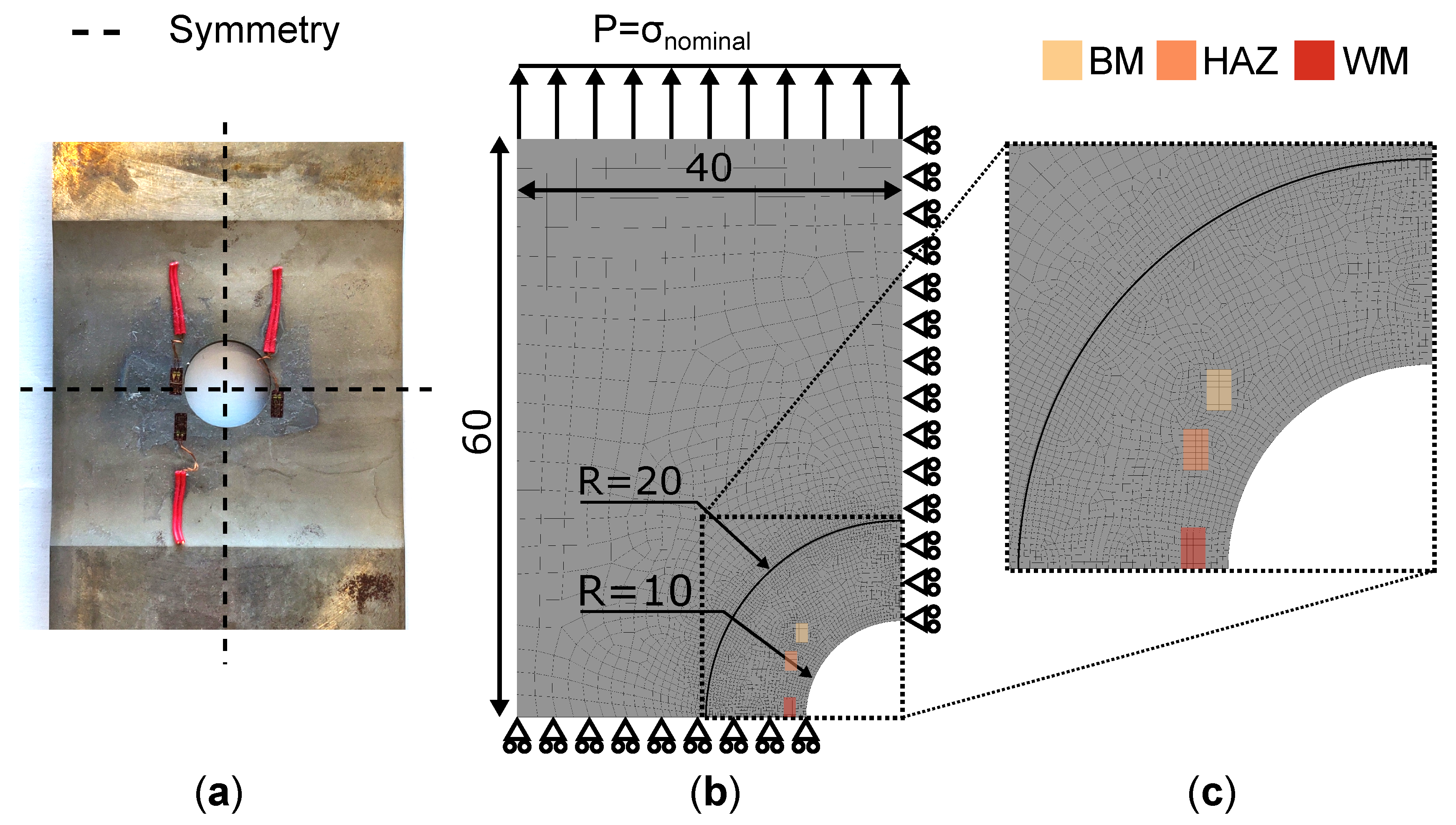
3.3. Finite Element Analysis

The V–C material model parameters were validated based on two criteria: estimation of the strain range per load cycle and estimation of the damage calculated using the Palmgren–Miner rule. Both criteria require replicating the axial strain measured during the validation experiments. The aim of the FEA is, therefore, to reproduce the validation experiments and to numerically estimate the axial strain recorded in each strain gauge.

The numerical study was conducted through ANSYS Workbench 2021 R2 [43]. The analysis was performed using a static structural analysis in ANSYS Mechanical and the geometry was created in SpaceClaim. The geometry was a replication of the test section of the validation specimen. Due to the nonlinear stress field caused by the validation specimen shape, two geometries, representative of the test sections of both validation specimens, were analyzed. These geometries considered the location of each strain gauge with respect to the stress concentration. The weld of the validation test specimen was not explicitly modeled. As the deformation in the test section was limited to the transition region between elastic and plastic deformation, it was assumed that the deformation in each material zone is mostly linear. On that account, the deformation in each material zone could be analyzed separately. Figure 6 presents the modeled geometry for specimen S690#1. The final geometry was a two-dimensional model, representative of a quarter of a test section, due to symmetry planes and plane strain assumption. The modeled test section was longer than the actual test section to avoid any effect of the boundary conditions on the strain results.

Each geometry was meshed using higher-order two-dimensional PLANE183 elements. The global mesh size was 3 mm. The mesh within an auxiliary arc was reduced to $0.3$ mm. This size guarantees a minimum of four elements along the shortest edge of each gauge area. A mesh convergence study showed that a coarser mesh would already show accurate results. The finer mesh was chosen to have additional nodal strain results in each strain gauge area and to have a uniform mesh. Finally, the mesh within each gauge area was mapped to create uniformly distributed quadrilateral elements. The smallest edges of any overlapping areas between two strain gauge areas were meshed with at least one element in the shortest direction to ensure that these features are properly modeled.

The boundary conditions for the geometry are shown in Figure 6b. Two symmetry boundary conditions were applied along the symmetry planes. To replicate the load as accurately as possible, the controlled nominal stress signal from each validation experiment was applied in the form of pressure boundary conditions. In total, 2100 load steps were applied. Four sub-steps were used in between each load step.

The material model was defined using the “isotropic elasticity” module, the “ nonlinear isotropic hardening Voce law” module, and the “Chaboche kinematic hardening” module. The “nonlinear isotropic hardening Voce law” implemented in ANSYS differs from the isotropic hardening law considered in this study (see Equation (1)) by a linear term $Q_0$.

$${\sigma }_y={\sigma }_{y0}+Q_0{\epsilon }_{eq}^p+Q_{\infty }\left(1-e^{-b{\epsilon }_{eq}^p}\right).$$

(10)

This expression can be reduced to Equation (1) by setting the linear coefficient $Q_0$ to zero.

Table 4. Summary of the V–C model parameters. The elastic modulus ${\mathrm{E}}_{\mathrm{opt}}$ is a result of the V–C model parameter optimization. The elastic modulus ${\mathrm{E}}_{\exp }$ is determined based on the material response. The Poisson’s ratio $\nu =0.3$ is used in each parameter set. The remaining parameters are the yield stress ${\sigma }_y$, the isotropic differential stress at saturation $Q_{\infty }$, the isotropic saturation rate parameter b, the kinematic stress parameter for the 1st and the 2nd backstress $C_1$ and $C_2$, and the corresponding kinematic saturation rate parameter ${\gamma }_1$ and ${\gamma }_2$.

Zone	${\mathit{E}}_{\mathbf{definition}}$	$\mathbf{E}$ [MPa]	${\mathit{\sigma }}_{\mathit{y}}$ [MPa]	${\mathit{Q}}_{\mathit{\infty }}$ [MPa]	b	${\mathit{C}}_1$ [MPa]	${\mathit{\gamma }}_1$	${\mathit{C}}_2$ [MPa]	${\mathit{\gamma }}_2$
WM	${\mathrm{E}}_{\mathrm{opt}}$	$\mathrm{176,515}$	596	$0.348$	$0.397$	$\mathrm{12,889}$	$105.405$	8685	$105.405$
WM	${\mathrm{E}}_{\exp }$	$\mathrm{204,000}$	571	$0.340$	$0.394$	$\mathrm{10,187}$	$100.365$	$\mathrm{16,296}$	$100.365$
HAZ	${\mathrm{E}}_{\mathrm{opt}}$	$\mathrm{178,448}$	608	$0.498$	$0.539$	$\mathrm{11,883}$	$96.204$	8725	$96.204$
HAZ	${\mathrm{E}}_{\exp }$	$\mathrm{208,000}$	586	$0.479$	$0.518$	8315	$105.299$	$\mathrm{18,649}$	$105.299$
BM	${\mathrm{E}}_{\mathrm{opt}}$	$\mathrm{196,844}$	694	$0.827$	$0.855$	$\mathrm{22,748}$	$656.594$	$\mathrm{25,851}$	$656.594$
BM	${\mathrm{E}}_{\exp }$	$\mathrm{209,000}$	728	$0.804$	$0.829$	$\mathrm{20,749}$	$459.169$	$\mathrm{20,749}$	$459.169$

summarizes each set of V–C model parameters used in the FEA. The Poisson’s ratio was set to $\nu =0.3$ for each set of parameters.

The axial strain was then obtained by the analyses, and was defined as the average nodal Green–Lagrange strain over each strain gauge area. The average nodal strain was calculated by summing the nodal strain values and dividing them by the number of nodes. The nodal strain was not weighted because the element size within the relevant areas was constant.

4. Results

4.1. V–C Model Parameter Estimation

Figure 7 presents the true stress–true strain results from the material model parameter estimation experiments for the load protocols “one cycle and tension until failure”. Noticeable differences in strain amplitude can be observed in the different material zones. For instance, the largest tensile strain was measured in the WM and the largest compressive strain was measured in the HAZ (see Figure 7b). The deformation in the BM was mainly elastic. In addition, although the strain applied over the entire test section (controlled by the extensometer) was fully reversed, the strain in each material zone (measured by a strain gauge) was not symmetric with respect to the origin. The extensometer covered the entire test section of the dog-bone specimens. As a result, the entire test section experienced fully-reversed loading, while the local deformation in each material zone depended on the local mechanical properties, on the size, and on the shape of the material zone. These local differences in deformation do not affect the model parameter optimization using the accumulated true strain approach.

Figure 8 presents selected experimental and numerical true stress–true strain results from the material model parameter estimation experiments. The individual plots highlight the influence of the elastic modulus on the elastic material response. The set of V–C model parameters with an optimized elastic modulus ${\mathrm{E}}_{\mathrm{opt}}$ consistently underestimated the elastic modulus of the considered material zone. Instead, the parameter set with a defined elastic modulus ${\mathrm{E}}_{\exp }$ captured the elastic material response more accurately. Nevertheless, the yield stress ${\sigma }_y$ was underestimated regardless of the definition of the elastic modulus. Each plot shows early yielding in the material response modeled using the V–C model. The values of the elastic modulus and the yield stress for each material zone are summarized in Table 4, together with the V–C model parameters.

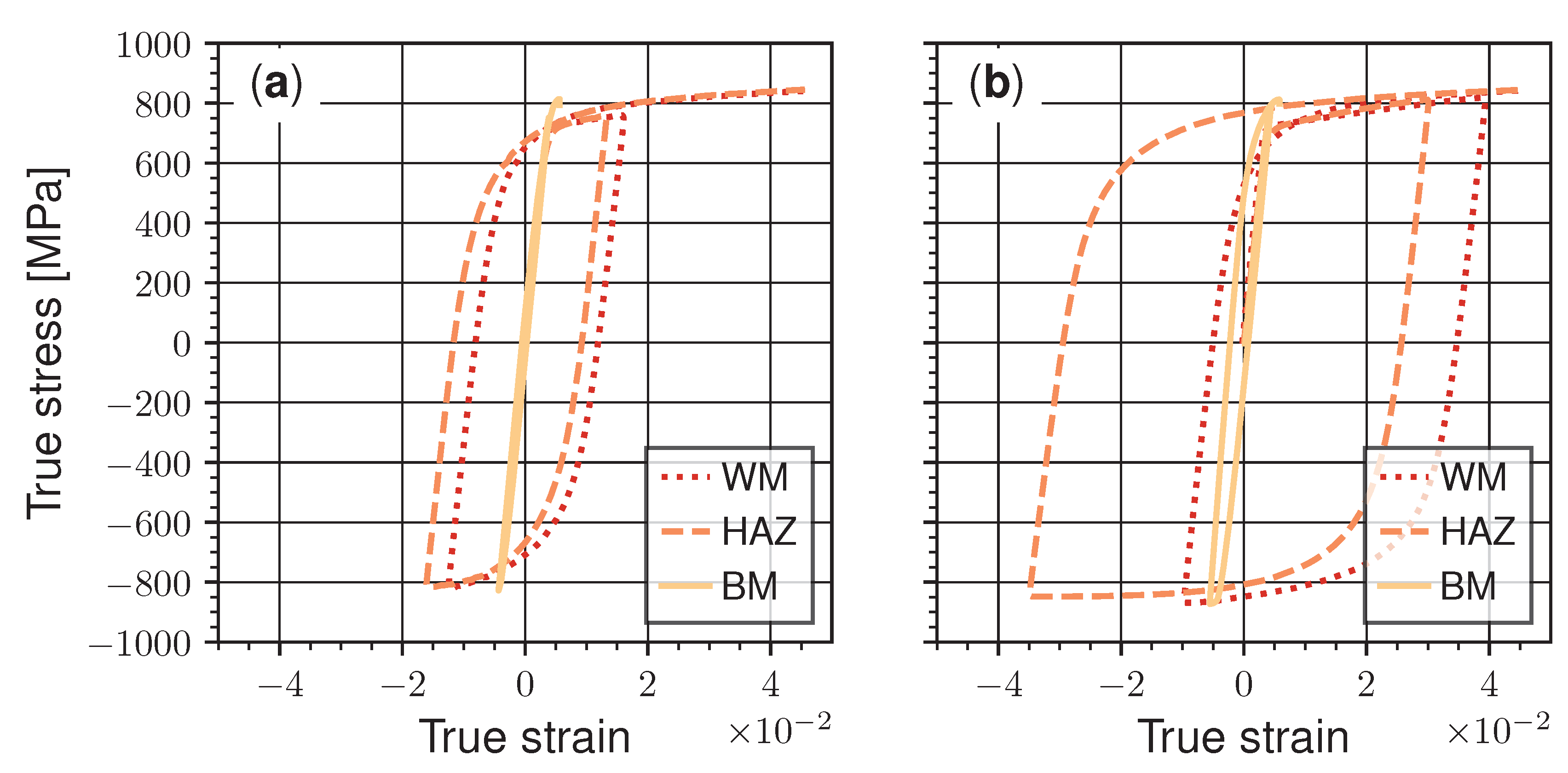
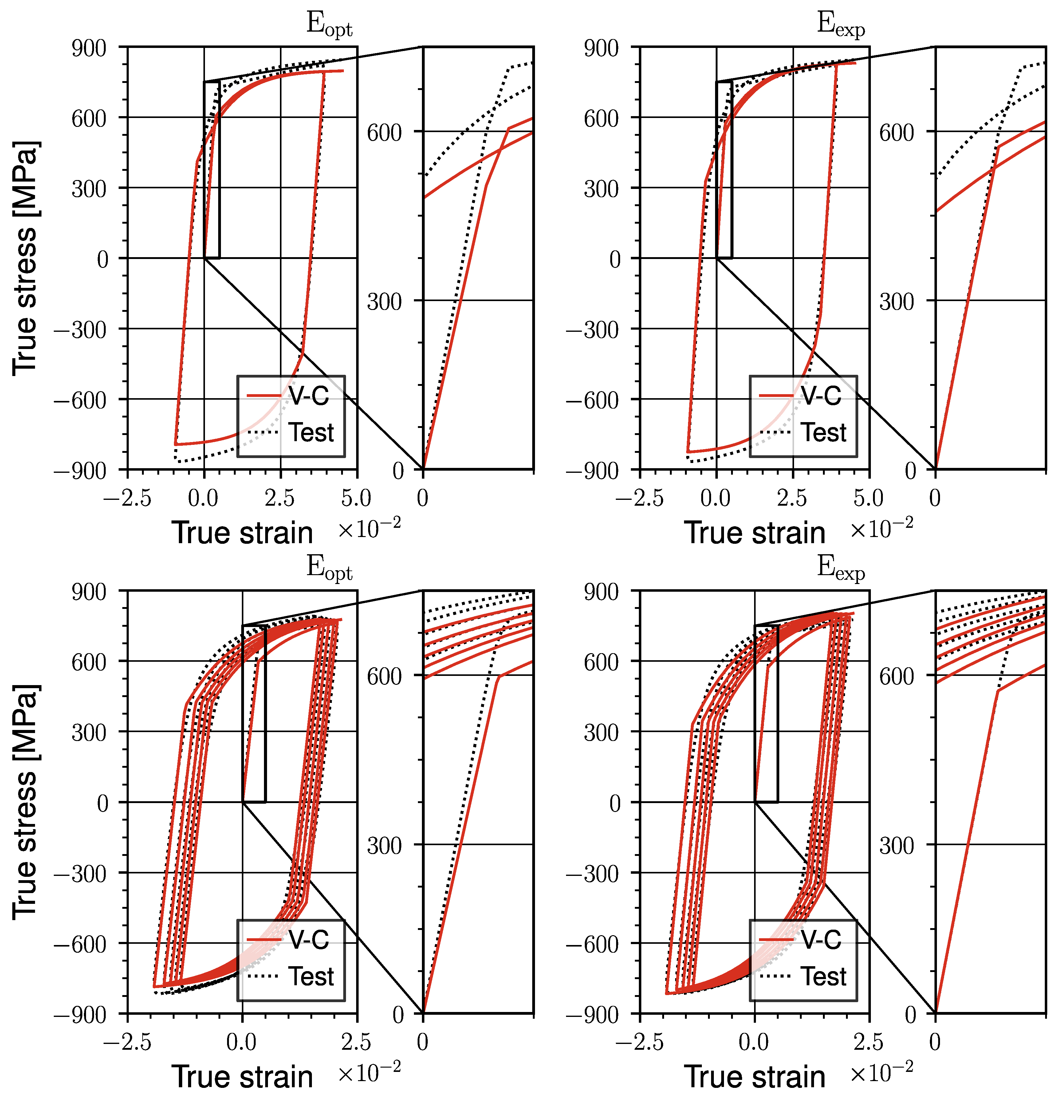
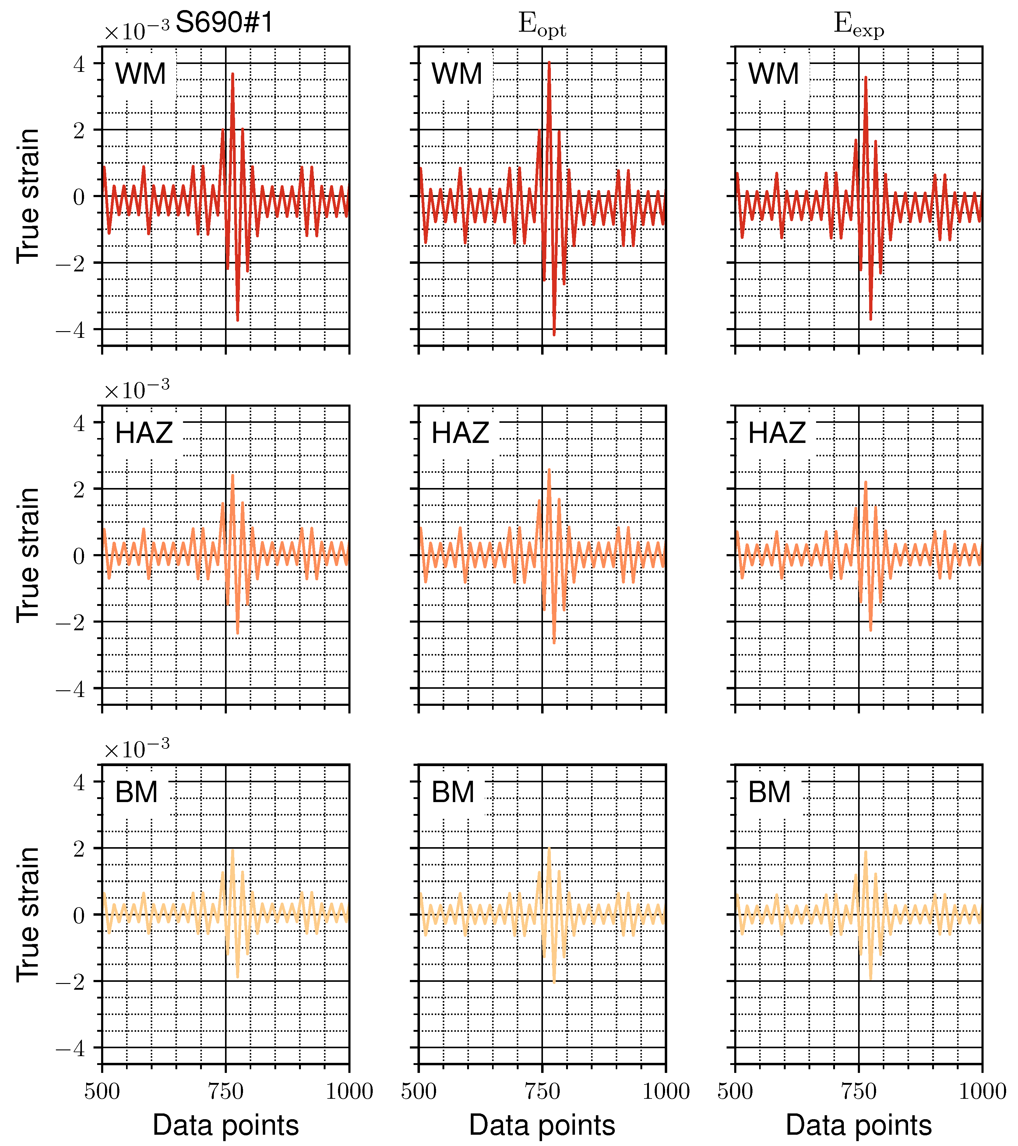
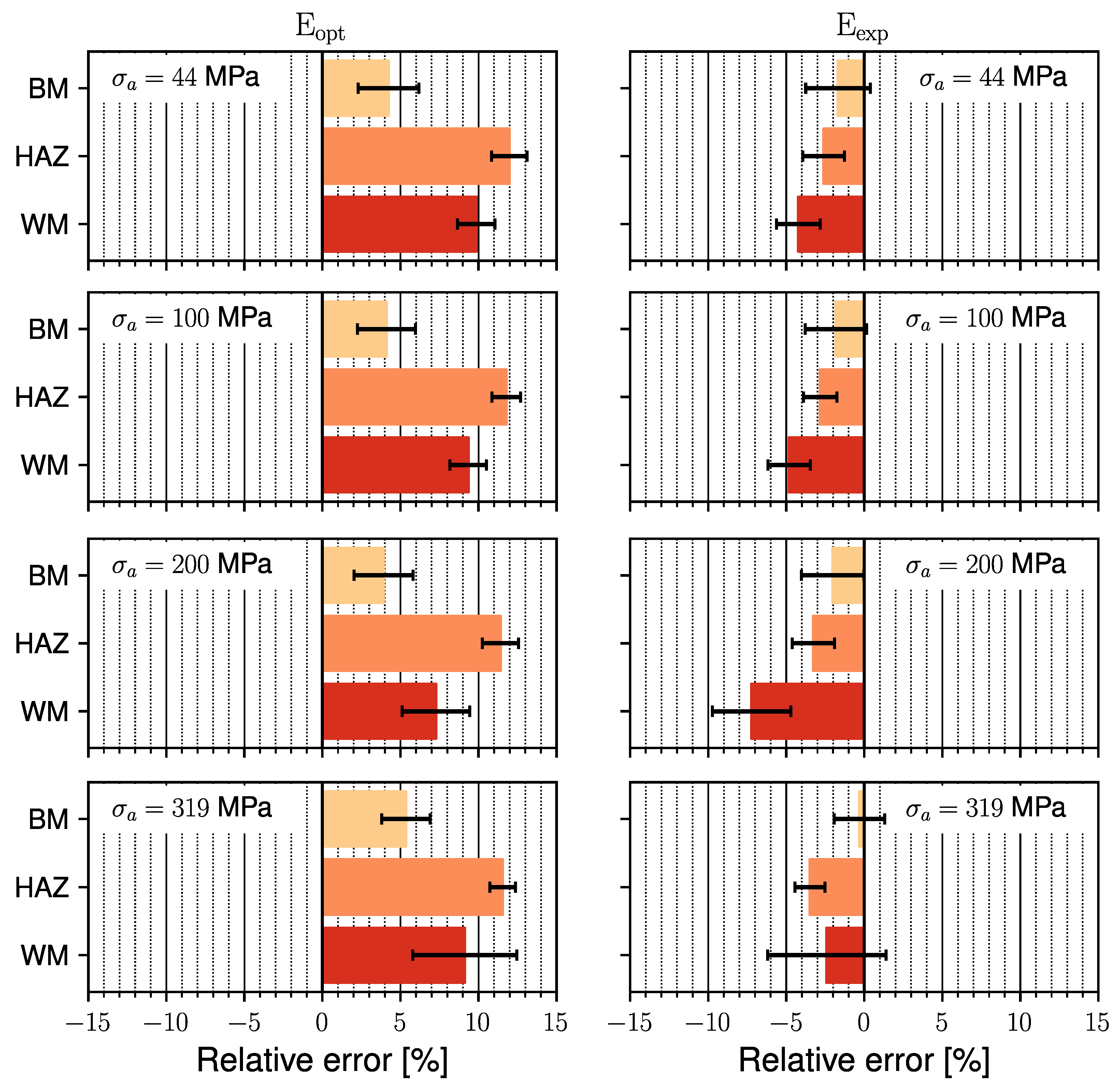
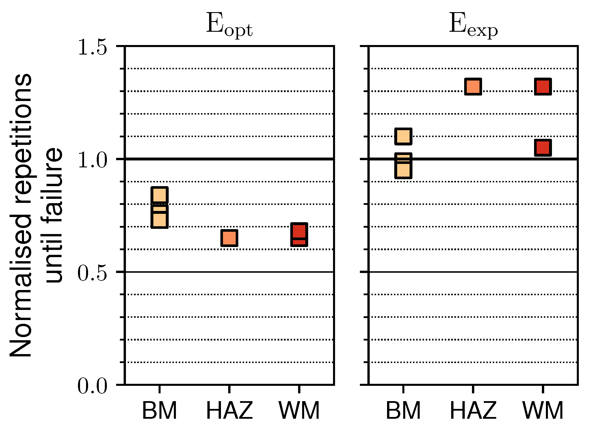
4.2. V–C Model Validation

The V–C model was validated using two different criteria: the relative error in the strain range per load cycle and the normalized number of load block repetitions until failure. These results were calculated for the first five repetitions of the validation load block (see Figure 5d). During the experiments, the HAZ strain gauge in specimen S690#2 was accidentally located in the BM. As a result, specimen S690#1 provided strain histories for the BM, the HAZ, and the WM, while specimen S690#2 provided two strain histories for the BM and one strain history for the WM.

Figure 9 presents a visual comparison of the strain recorded during the validation experiments and the corresponding numerical strain result. Firstly, this figure highlights the differences in strain amplitude between different material zones. The highest strain was measured in the WM since the WM strain gauge was located close to the location of the largest stress concentration. Moreover, the WM has the lowest hardness and is prone to plastic deformation. Secondly, this figure shows that the strain estimated using the V–C model parameter set with the optimized elastic modulus ${\mathrm{E}}_{\mathrm{opt}}$ led to an overestimation of the strain amplitude. This observation agrees with previous results. Thirdly, a difference in mean strain between the experimental and numerical strain results was observed in the WM.

It should be noted that, although the applied load was fully reversed (in the validation experiments), the deformation in each material zone was not due to their different mechanical properties. The resulting asymmetric loading allowed ratcheting strain to develop. In the numerical results, ratcheting was likely caused by dissimilar isotropic and kinematic hardening rates at different locations in the test specimen. Since the stress field created by the shape of the validation specimen was nonlinear, only some areas in the test specimen experienced plastic deformation, leading to cyclic hardening or softening. This local change in mechanical properties likely led to the presence of a mean stress. As a result, a ratcheting strain could develop. Nonetheless, the ratcheting strain, present in the experimental and numerical strain results, was small compared to the strain amplitude and did not affect the model validation.

The average relative error was calculated for the strain range of each load cycle of a certain load level in the validation load protocol. Here, load cycle refers to the fully-reversed load cycles in the validation load block. The strain range of each load cycle was defined as $\mathsf{\Delta }\epsilon ={\epsilon }_{\max }-{\epsilon }_{\min }$. The relative error per load cycle was defined as

$$e_{\mathrm{rel}}[\%]=100\times \frac{\mathsf{\Delta }{\epsilon }_{\mathrm{FEA}}-\mathsf{\Delta }{\epsilon }_{\mathrm{experiment}}}{\mathsf{\Delta }{\epsilon }_{\mathrm{FEA}}}.$$

(11)

Finally, the relative error was averaged over the number of cycles at a certain load level. Since only the first five repetitions of the validation load protocol were considered, this amounted to 60 load cycles at the stress amplitude ${\sigma }_a=44$ MPa, 30 load cycles at ${\sigma }_a=100$ MPa, 10 load cycles at ${\sigma }_a=200$ MPa, and 5 load cycles at ${\sigma }_a=319$ MPa.

Figure 10 presents the average relative error per load level. The set of V–C model parameters with an optimized elastic modulus ${\mathrm{E}}_{\mathrm{opt}}$ consistently overestimated the strain range for each applied stress amplitude. The relative error was constant across the different applied stress amplitudes ${\sigma }_a$ in the BM and the HAZ. The relative error of the WM decreased noticeably at ${\sigma }_a=200$ MPa. The set of V–C model parameters with an experimentally determined elastic modulus ${\mathrm{E}}_{\exp }$ underestimated the strain range for each applied load amplitude, but it also shows smaller relative errors compared to the optimized set. The largest relative error was observed in the WM at ${\sigma }_a=200$ MPa. The relative error of the HAZ increased with increasing applied stress amplitude.

When the deformation is elastic, the relative error in each material zone is constant, as it only depends on the chosen elastic modulus. At an applied stress amplitude of ${\sigma }_a=200$ MPa, the WM experienced almost three times higher stresses due to the stress concentration effect of the hole in the specimen. At these stress levels, the WM is about to yield. Since the yield stress used by the V–C model is lower than the experimentally determined offset yield stress of the WM, the numerical result starts to deviate from the experimental result. The relative error reduces at ${\sigma }_a=319$ MPa, as both the experimentally measured strain and the numerically simulated strain include plasticity. Considering the relative error within the same material zones under different stress amplitude, the differences in the relative error have high variability for the experimentally determined elastic modulus ${\mathrm{E}}_{\exp }$. The V–C model with an optimized elastic modulus ${\mathrm{E}}_{\mathrm{opt}}$ sacrifices some accuracy in the elastic material response for better accuracy when the material response is predominately plastic [15].

Finally, the standard deviation ${\sigma }_{\mathrm{SD}}$ of the relative error, presented by the error bar, shows the variability in experiments, strain gauge location, and measurement-accuracy-related limitations. The cycling frequency and the sampling frequency used during the validation experiments led to a slight delay between the recorded force and the recorded strain signal. This delay was especially noticeable at the highest load level due to the high loading speed. The resulting uncertainty about the timing of the strain measurement around the peak load led to a larger standard deviation.

To analyze the influence of the difference in strain range on the fatigue life estimation, the number of repetitions until failure of the first five repetitions of the validation load protocol was determined for the experimental and numerical strain histories. The number of repetitions until failure was calculated using the Palmgren–Miner damage $D_{\mathrm{load}\mathrm{history}}$,

$$B_{f,\mathrm{load}\mathrm{history}}=\frac{1}{D_{\mathrm{load}\mathrm{history}}}.$$

(12)

To calculate the damage $D_{\mathrm{load}\mathrm{history}}$, the closed load cycles within the load history were extracted using the rainflow-counting algorithm. Rainflow-counting was performed on the stress signal since the same stress was applied during the experiments and in the FEA. For each closed load cycle, the number of cycles until failure $N_f$ was estimated using the mean stress-corrected strain–life equation,

$${\sigma }_{\max }{\epsilon }_a^{\mathrm{tot}}=\frac{{\left({\sigma }_f^{\prime }\right)}^2}{\mathrm{E}}{\left(N_f\right)}^{2b}+{\sigma }_f^{\prime }{\epsilon }_f^{\prime }{\left(N_f\right)}^{b+c}.$$

(13)

The coefficients ${\sigma }_f^{\prime }$, ${\epsilon }_f^{\prime }$, b, and c were estimated based on the hardness results. The coefficients were ${\sigma }_f^{\prime }=1317$ MPa and ${\epsilon }_f^{\prime }=0.39$ for the BM, ${\sigma }_f^{\prime }=1317$ MPa and ${\epsilon }_f^{\prime }=0.40$ for the HAZ, and ${\sigma }_f^{\prime }=1249$ MPa and ${\epsilon }_f^{\prime }=0.43$ for the WM. The remaining coefficients b and c were set to $-0.09$, and $-0.56$, respectively, for each material zone. The elastic modulus $\mathrm{E}$ was defined as ${\mathrm{E}}_{\exp }$. The values ${\sigma }_{\max }$ and ${\epsilon }_a^{\mathrm{tot}}$ were extracted from the load histories using rainflow-counting. The number of cycles until failure $N_f$ was calculated for each closed cycle within the load history by solving the strain–life equation numerically. Once the resulting number of repetitions until failure of each experimental and numerical load history $B_{f,\mathrm{load}\mathrm{history}}$ were known, the numerical results were normalized with the experimental results, $B_{f,\mathrm{FEA}}/B_{f,\mathrm{experiment}}$.

Figure 11 presents the average normalized repetitions until failure. The sets of V–C model parameters with an optimized elastic modulus ${\mathrm{E}}_{\mathrm{opt}}$ led to conservative damage estimates. Previous results showed that this set of V–C model parameters overestimates the strain range (see Figure 10). The overestimated error per load cycle was accumulated in the damage calculation, which led to conservative fatigue life estimates. The sets of V–C model parameters with an experimentally determined elastic modulus ${\mathrm{E}}_{\exp }$ led to non-conservative results, as this set of model parameters tended to underestimate the strain range. Nonetheless, these non-conservative damage estimates were closer to the expected experimental values.

5. Discussion

As summarized in the literature review presented in Section 1, multiple studies have been conducted on the estimation of the V–C model parameters. These studies have focused on determining the best V–C model parameters to model large deformation. Although the V–C model is extensively used to model a wide range of cyclic loads, Agius et al. [19] and other authors pointed out that there is no consensus on how to define the V–C model parameters. The parameter identification is subjected to uncertainty, and the process can be time-consuming. In addition to that, modeling the deformation of welded joints presents a unique challenge due to differences in the mechanical properties of each material zone. Some material zones may experience plastic deformation, while others are still deforming elastically. In applications where the total deformation of the weld leads to local strains in the transition region between elastic and plastic strain, it is crucial that the chosen material model estimates both the elastic and the plastic material response accurately.

The current study focuses on the V–C model parameter identification in the transition region between the elastic and the plastic strain. Indeed, welded joints in high-strength marine structures are expected to experience strain limited to this transition region. The fit of the V–C model parameters is assessed by comparing the numerical stress–strain results to experimental stress–strain results. Special attention is given to the definition of the elastic modulus because this parameter defines how elastic deformation is modeled. To the best of the authors’ knowledge, only Agius et al. [19] have conducted a similar study. In that work, the authors systematically determined the V–C model parameters for aluminum alloy AA 7075-T6 by using a multi-objective genetic algorithm.

The results demonstrate that the accumulated true strain approach, as implemented in the Python library RESSPyLab, was used successfully to estimate the V–C model parameters for each material zone of a butt-welded joint made from S690 steel. The input stress and strain histories were collected from a dog-bone specimen with a weld in the test section. This test specimen design reduced the required number of cyclic tests by a factor of three compared to the original methodology in [15], as one test specimen was sufficient to collect input data for three different material zones. These stress–strain histories were also used to estimate the elastic modulus of each material zone and the offset yield strength of the material zones with the lowest hardness.

The V–C model parameter estimation process seems to systematically underestimate the yield strength of each material zone to achieve a better accuracy in modeling the cyclic material response [15]. Moreover, the definition of the elastic modulus within each set of V–C model parameters has a noticeable effect on the capability to represent the strain response. When the elastic modulus is defined by the optimization algorithm, it is lower than the expected experimental value. A lower elastic modulus leads to an overestimated elastic strain. Since the strain range considered in this study was focused on the transition region where plastic strain is limited, a lower elastic modulus also leads to an overestimated total strain. In addition, any error in strain estimation is accumulated during the calculation of the fatigue life, since the Palmgren–Miner damage rule was used. As a result, an overestimated total strain leads to a conservative fatigue life estimate. In this study, fatigue life estimation was improved by defining the elastic modulus based on tensile tests. This reduced the relative error in the strain range estimation by up to 9%, resulting in better, yet non-conservative, fatigue life results. Based on this observation, it is recommended to exclude the elastic modulus from the parameter estimation, albeit the resulting fatigue life estimation is non-conservative.

Although the present study successfully estimated the V–C model parameters and validated the V–C model using a relevant load profile, some limitations should be addressed. Firstly, the strain-controlled load protocols used in the V–C model parameter estimation experiment did not lead to fully-reversed cyclic loading. The dissimilar end levels of the applied strain led to the development of ratcheting strains in each material zone. The ratcheting strains did not affect the results of this study because only the short-term material response was considered in the V–C model parameter estimation and the model validation. Nonetheless, the development of ratcheting strains can be avoided by performing the material model parameter estimation experiments separately for each material zone. These test specimens should also be used if fatigue crack initiation is expected in the material zone with the highest hardness. Secondly, the validation experiments were performed using only two test specimens and only one load history. Additional load protocols with higher load levels and additional validation load histories should be considered. Lastly, it is essential to define a material model that can account for any change in the stress–strain behavior after an overload, e.g., when a ship navigates through a storm. Thus, future research should investigate the ability of the V–C model to estimate the long-term strain response in the presence of overloads. Current understanding suggests that it is not possible to model memory effects [17]. However, these studies should be revisited for load histories with load levels limited to the transition region between elastic and plastic strain.

6. Conclusions

This paper applied the V–C material model to welded high-strength steel joints subjected to fatigue-relevant loads in large ship structures. The V–C model parameters were determined using the NTR-based accumulated true strain approach developed by de Castro e Sousa et al. [15]. The stress–strain histories, required to determine the V–C model parameters for each material zone, were sampled from a tensile test coupon with a weld in the test section. The material model was validated by comparing the results from load-controlled variable amplitude cyclic loading experiments to numerical results from an FEA.

Based on the results, it was found that the NTR-based accumulated true strain approach could be used to determine the V–C model parameters for different material zones in a welded joint. The elastic modulus used in the V–C model should be defined based on uniaxial tensile tests instead of being optimized as a V–C model parameter. The optimization algorithm proposed by de Castro e Sousa et al. [15] tends to underestimate the elastic modulus and the yield strength, resulting in an overestimated total strain. As the strain in welded joints in marine structures is often limited to the transition region between elastic and plastic strain, the proper definition of the elastic material response is fundamental to improving strain–life estimation.

References

1. Mancini, F.; Remes, H.; Romanoff, J.; Gallo, P. Influence of weld rigidity on the non-linear structural response of beams with a curved distortion. Eng. Struct. 2021, 246, 113044. [Google Scholar] [CrossRef]
2. Tailored Products. Available online: https://www.meyerwerft.de/en/technologies/tailored_products/index.jsp (accessed on 9 March 2022).
3. Gallo, P.; Remes, H.; Romanoff, J. Influence of crack tip plasticity on the slope of fatigue curves for laser stake-welded T-joints loaded under tension and bending. Int. J. Fatigue 2017, 99, 125–136. [Google Scholar] [CrossRef]
4. Gallo, P.; Guglielmo, M.; Romanoff, J.; Remes, H. Influence of crack tip plasticity on fatigue behaviour of laser stake-welded T-joints made of thin plates. Int. J. Mech. Sci. 2018, 136, 112–123. [Google Scholar] [CrossRef] [Green Version]
5. Liinalampi, S.; Remes, H.; Lehto, P.; Lillemäe, I.; Romanoff, J.; Porter, D. Fatigue strength analysis of laser-hybrid welds in thin plate considering weld geometry in microscale. Int. J. Fatigue 2016, 87, 143–152. [Google Scholar] [CrossRef]
6. Remes, H.; Korhonen, E.; Lehto, P.; Romanoff, J.; Niemelä, A.; Hiltunen, P.; Kontkanen, T. Influence of surface integrity on the faitgue strength of high strength steels. J. Constr. Steel Res. 2013, 89, 21–29. [Google Scholar] [CrossRef]
7. Hobbacher, A.F. Recommendations for Fatigue Design of Welded Joints and Components; doc. XIII-2151r4-07/XV-1254r4-07; International Institute of Welding: Paris, France, 2008. [Google Scholar]
8. Remes, H.; Gallo, P.; Jelovica, J.; Romanoff, J.; Lehto, P. Fatigue strength modeling of high-performing welded joints. Int. J. Fatigue 2020, 135, 105555. [Google Scholar] [CrossRef]
9. Devaney, R.J.; O’Donoghue, P.E.; Leen, S.B. Effect of welding on microstructure and mechanical response of X100Q bainitic steel through nanoindentation, tensile, cyclic plasticity and fatigue characterization. Mater. Sci. Eng. A 2021, 804, 140728. [Google Scholar] [CrossRef]
10. Hemmesi, K.; Holey, H.; Elmoghazy, A.; Böhm, R.; Farajian, M.; Schulze, V. Modeling and experimental validation of material deformation at different zones of welded structural-steel under multiaxial loading. Mater. Sci. Eng. A 2021, 824, 140826. [Google Scholar] [CrossRef]
11. Garcia, M.A.R. Multiaxial Fatigue Analysis of High Strength Steel Welded Joints Using Generalizied Local Approaches. Ph.D. Thesis, École Polytechnique Fédérale de Lausanne, Lausanne, Switzerland, 4 September 2020. [Google Scholar]
12. Song, W.; Liu, X.; Xu, J.; Fan, Y.; Shi, D.; Khosravani, M.R.; Berto, F. Multiaxial low cycle fatigue of notched 10CrNi3MoV steel and its undermatched welds. Int. J. Fatigue 2021, 150, 106309. [Google Scholar] [CrossRef]
13. Chukkan, J.R.; Wu, G.; Fitzpatrick, M.E.; Eren, E.; Zhang, X.; Kelleher, J. Residual stress redistribution during elastic shake down in welded plates. MATEC Web Conf. 2018, 165, 21004. [Google Scholar] [CrossRef]
14. Ono, Y.; Yıldırım, H.C.; Kinoshita, K.; Nussbaumer, A. Damage-based assessment of the fatigue rack initiation site in high strength steel welded joints treated by HFMI. Metals 2022, 12, 145. [Google Scholar] [CrossRef]
15. de Castro e Sousa, A.; Suzuki, Y.; Lignos, D.G. Consistency in solving the inverse problem of the Voce-Chaboche constitutive model for plastic straining. J. Eng. Mech. 2020, 146, 04020097. [Google Scholar] [CrossRef]
16. Hartloper, A.R.; de Castro e Sousa, A.; Lignos, D.G. Constitutive modeling of structural steels: Nonlinear isotropic/kinematic hardening material model and its calibration. J. Struct. Eng. 2021, 147, 04021031. [Google Scholar] [CrossRef]
17. Court-Patience, D.; Garnich, M. FEA strategy for realistic simulation of buckling-restraint braces. J. Struct. Eng. 2021, 147, 04021186. [Google Scholar] [CrossRef]
18. Koo, G.-H.; Ahn, S.-W.; Hwang, J.-K.; Kim, J.-S. Shaking table tests to validate inelastic seismic analysis method applicable to nuclear metal components. Appl. Sci. 2021, 11, 9264. [Google Scholar] [CrossRef]
19. Agius, D.; Kajtaz, M.; Kourousis, K.I.; Wallbrink, C.; Wang, C.H.; Hu, W.; Silva, J. Sensiticity and optimization of the Chaboche plasticity model parameters in strain-life fatigue predictions. Mater. Des. 2017, 118, 107–121. [Google Scholar] [CrossRef] [Green Version]
20. Chaboche, J.L.; Dang Van, K.; Cordier, G. Modelization of the strain memory effect on the cyclic hardening of 316 stainless steel. In Proceedings of the Transactions of the International Conference on Structural Mechanics in Reactor Technology, Berlin, Germany, 13–21 August 1979. [Google Scholar]
21. Bari, S.; Hassan, T. Anatomy of coupled constitutive models for ratcheting simulation. Int. J. Fatigue 2000, 16, 381–409. [Google Scholar] [CrossRef]
22. Nip, K.H.; Gardner, L.; Davies, C.M.; Elghazouli, A.Y. Extremely low cycle fatigue tests on structural carbon steel and stainless steel. J. Constr. Steel Res. 2010, 66, 96–110. [Google Scholar] [CrossRef]
23. Lee, C.; Do, V.; Chang, K. Analysis of uniaxial ratcheting behavior and cyclic mean stress relaxation of a duplex stainless steel. Int. J. Plasticity 2014, 62, 17–33. [Google Scholar] [CrossRef]
24. Chaboche, J.L. Time-independent constitutive theories for cyclic plasticity. Int. J. Fatigue 1986, 2, 149–188. [Google Scholar] [CrossRef]
25. Smith, C.; Kanvinde, A.; Deierlein, G. Calibration of Continuum Cylic Constitutive Models for Structural Steel Using Particle Swarm Optimization. J. Eng. Mech. 2017, 143, 04017012. [Google Scholar] [CrossRef]
26. Rezaiee-Pajand, M.; Sinaie, S. On the calibration of the Chaboche hardening model and a modified hardening rule for uniaxial ratcheting prediction. Int. J. Solids Struct. 2009, 46, 3009–3017. [Google Scholar] [CrossRef] [Green Version]
27. Pal, S.; Wije Wathugala, G.; Kundu, S. Calibration of a constitutive model using genetic algorithms. Comput. Geotech. 1996, 19, 325–348. [Google Scholar] [CrossRef]
28. Nath, A.; Barai, S.V.; Ray, K.K. Studies on the experimental and simulated cyclic-plasticity response of structural mild steels. J. Constr. Steel Res. 2021, 182, 106652. [Google Scholar] [CrossRef]
29. RESSPyLab 1.1.6. Available online: https://pypi.org/project/RESSPyLab/ (accessed on 15 February 2022).
30. Voce, E. The relationship between stress and strain for homogeneous deformations. J. Inst. Met. 1948, 74, 537–562. [Google Scholar]
31. Armstrong, P.J.; Frederick, C.O. A mathematical representation of the multiaxial Bauschinger effect. Mater. High Temp. 2007, 24, 1–26. [Google Scholar]
32. ISO 1099:2006(E); Metallic Materials—Vickers Hardness Test—Part 1: Test Method. International Organization for Standardization: Geneva, Switzerland, 2018.
33. Boyer, H.E.; Gall, T.L. Metals Handbook, Desk edition; ASM Materials: Park Ohio, OH, USA, 1985; p. 1500. [Google Scholar]
34. Roessle, M.L.; Fatemi, A. Strain-controlled fatigue properties of steels and some simple approximations. Int. J. Fatigue 2000, 22, 495–511. [Google Scholar] [CrossRef]
35. E 606M-04; Standard Practice for Strain-Controlled Fatigue Testing. ASTM International: West Conshohocken, PA, USA, 2005.
36. Petry, A. Nonlinear Material Modelling for Fatigue Life Prediction of Welded Joints in High Strength Marine Structures. Master’s Thesis, Master of Science in Technology, Aalto University, Espoo, Finland, 1 February 2022. [Google Scholar]
37. DNV. Fatigue Assessment of Ship Structures; DNv-cG-0129; DNV: Høvik, Norway, 2021. [Google Scholar]
38. Hales, R.; Holdsworth, S.R.; O’Donnell, M.P.; Perrin, I.J.; Skelton, R.P. A Code of Practice for the determination of cyclic stress-strain data. Mater. High Temp. 2002, 19, 165–185. [Google Scholar] [CrossRef]
39. ISO 12106:2003(E); Metallic Materials—Fatigue Testing—Axial-Strain-Controlled Method. International Organization for Standardization: Geneva, Switzerland, 2003.
40. ISO 1099:2006(E); Metallic Materials—Fatigue Testing—Axial Force-Controlled Method. International Organization for Standardization: Geneva, Switzerland, 2006.
41. Savitzky, A.; Golay, M.J. Smoothing and differentiation of data by simplified least squares procedures. Anal. Chem. 2002, 36, 1627–1639. [Google Scholar] [CrossRef]
42. E 8M-04; Standard Test Methods for Tension Testing of Metallic Materials [Metric]. ASTM International: West Conshohocken, PA, USA, 2003.
43. ANSYS Student 2021 R2; ANSYS, Inc.: Canonsburg, PA, USA, 2021; Available online: https://www.ansys.com/academic/students/ansys-student (accessed on 17 March 2022).
Figure 1. Macro sample of the welded S690 steel with micro hardness indentations: (a) annotated macro sample, (b) corresponding hardness profile.
Jmse 10 00818 g001
Figure 2. Test specimen used in the material model parameter estimation experiments: (a) dimensions of the dog-bone specimen, and (b) manufactured dog-bone specimen. The dimensions are provided in mm unless stated differently. The schematic is not drawn to scale.
Jmse 10 00818 g002
Figure 3. Test specimen used in the validation experiments: (a) dimensions of the flat specimen, and (b) manufactured flat specimen. The dimensions are provided in mm unless stated differently. The schematic is not drawn to scale.
Jmse 10 00818 g003
Figure 4. Experimental test setup used in the material model parameter estimation experiments and the validation experiments: (a) MTS-810 test system with a dog-bone specimen specimen, (b) instrumented dog-bone specimen with extensometer, (c) MTS-370.50 test system with a flat specimen, (d) instrumented flat specimen.
Jmse 10 00818 g004
Figure 5. Load profiles for the material parameter estimation experiments and the validation experiment: (a) one cycle and tension until failure, (b) constant amplitude cycling, (c) incremental step test, (d) validation.
Jmse 10 00818 g005
Figure 6. Overview of the different activities of the validation experiment. (a) Photo of validation test specimen S690#1. (b) Overview of the finite element analysis model used to replicate the validation results. This schematic shows the dimensions of the geometry, the boundary conditions, and the final mesh. The geometry is reduced to a two-dimensional geometry using a plane strain assumption. (c) Mesh refinement around the circular notch. The positions of the strain gauges are highlighted in color.
Jmse 10 00818 g006
Figure 7. True stress–true strain hysteresis loops recorded during the V–C model parameter estimation experiments: (a) Specimen 2, ε a = 1.0 %, and (b) specimen 1, ε a = 2.0 %. The strain was only recorded up to ε = 5 %.
Jmse 10 00818 g007
Figure 8. Selected material model parameter estimation results and the corresponding V–C model for the WM. The plots highlight the differences in the elastic material response based on the choice of elastic modulus ( E opt or E exp ).
Jmse 10 00818 g008
Figure 9. Visual comparison between the measured and simulated (V–C) strain signal of the validation experiment. The strain results correspond to specimen S690#1. Differences in the mean strain are caused by the development of ratcheting strain during the physical and numerical experiments.
Jmse 10 00818 g009
Figure 10. The average relative error in strain range estimation. The standard deviation of the relative error is presented using error bars. A negative relative error indicates that the V–C model underestimates the strain range, while a positive relative error indicates that the V–C model overestimates the strain range. The number of stress–strain signals considered for each material are n = 3 for the BM, n = 1 for the HAZ, and n = 2 for the WM.
Jmse 10 00818 g010
Figure 11. Normalized repetitions until failure for each material zone calculated using the Palmgren–Miner damage rule and the mean stress corrected strain–life equation. A normalized result of less than 1.0 indicates a conservative result, while a result above one 1.0 indicates a non-conservative result.
Jmse 10 00818 g011