
Research on AUV Energy Saving 3D Path Planning with Mobility Constraints


Laboratory of Science and Technology on Underwater Vehicle, Harbin Engineering University, Harbin 150001, China
*
Author to whom correspondence should be addressed.
J. Mar. Sci. Eng. 2022, 10(6), 821; https://0-doi-org.brum.beds.ac.uk/10.3390/jmse10060821
Submission received: 28 April 2022
/
Revised: 10 June 2022
/
Accepted: 12 June 2022
/
Published: 15 June 2022
(This article belongs to the Special Issue Autonomous Underwater Vehicle Technology Advances in Ocean Observation)
Abstract
:This paper aims to focus on the path planning problem of AUV in the marine environment. As well as considering the path length and safe obstacle avoidance, ocean currents should not be ignored as the main factor affecting the navigation energy consumption of AUV. At the same time, the path should satisfy the mobility constraint of AUV; otherwise, the path is inaccessible to AUV. For the above problems, this paper presents a path planning algorithm based on an improved particle swarm (EPA-PSO); the fitness function is designed based on path length, energy consumption, and mobility constraints. The updated law of particle velocity and the initialization law of particles are improved, and the possible optimal solutions are stored in the feasible solution set; finally, the optimal solutions are obtained by comparison. The local jumping ability is given to the particle swarm so that the particles can jump out of the local optimal solution. The path planning simulation experiment is compared with the traditional PSO algorithm. The results show that the EPA-PSO algorithm proposed in this paper can be used in the AUV three-dimensional path planning process. It can effectively save energy and make the navigation path of AUV satisfy the requirements of maneuverability. The field experiment was completed in Shanghai, China, and the experiment proved that it was feasible to obtain a path satisfying the maneuverability constraints with optimal energy consumption for the problems studied in this paper.
1. Introduction
With further exploration of the marine environment, there are still many areas that cannot be touched by humans. An autonomous underwater robot (AUV) is a better tool to explore the ocean instead of human beings. At present, AUV has played an important role in the exploration of the marine environment [1], military combat support [2], submarine pipeline detection [3] and other aspects. An excellent path planning system is the prerequisite for AUV to perform tasks [4]; however, a complex marine environment will make it difficult for AUV to perform underwater tasks sharply. The quality of the planned path will directly have a huge impact on the efficiency of AUV’s task execution and AUV’s safety. With the development of science and technology at the present stage, scholars have developed more and more path planning algorithms, such as Dijkstra [5] algorithm, A* [6] algorithm, artificial potential field method [7], RRT [8] algorithm, and other algorithms, which are applied in the field of AUV.
In the three-dimensional environment with irregular obstacles and ocean currents, the traditional graph search path planning algorithm has the disadvantage of large computation in high latitude space [9], which is obviously not suitable. At the same time, when the planned path has the characteristics of a large depth span and short horizontal sailing distance, the planned path may be difficult to reach by ignoring the mobility constraints of the AUV, which will also increase the risk of AUV performing tasks. Therefore, the planning process should pay more attention to the mobility requirements of AUV. Maneuverability constraints of AUV in a three-dimensional environment are more complex than those in constant depth. To keep the attitude stability of AUV, not only the rotation limit of AUV should be considered, but also the pitch angle of AUV should be kept within a certain range. At the same time, due to the limited onboard energy of AUV, ocean currents will also have a great impact on the energy consumption of AUV. Considering the energy consumption in the planning process can improve the endurance of AUV and extend the service life of AUV. To sum up, in the process of AUV 3D path planning, a path that can save energy and satisfy the requirements of mobility is of great significance to the completion of follow-up tracking tasks and control processes. Swarm intelligence algorithm has the advantages of easy implementation, high precision and fast convergence [10], which has attracted extensive attention in the academic circles and has shown its advantages in solving practical problems.
At present, scholars have also made great achievements in AUV energy-saving path planning. AUV energy-saving path planning can be studied in two ways. One method is to reduce energy consumption through the rational use of ocean currents, and the other method is to develop energy-saving algorithms. Teong Beng Koay et al. [11] proposed the motion strategy of using ocean currents to maximize the use of favorable ocean currents while minimizing the use of propulsion force. In this way, the energy consumption of the propulsion system can be reduced to achieve the purpose of energy conservation. PENG YAO [12] applied the improved Interferometric Fluid Dynamic System (IIFDS) to AUV 3D path planning in an environment with complex static obstacles, ocean currents, and dynamic threats. By leading into the weight coefficient of the flow field, the algorithm can balance the path length and flow utilization rate. IIFDS combined with the reverse avoidance strategy can obtain a feasible path when there is a simple dynamic threat in the environment. However, the paths obtained in the above studies are all downstream navigation paths as far as possible, which is very unfavorable for AUV jointly controlled by rudder OARS. Downstream will significantly reduce the rudder efficiency of AUV, thus affecting the maneuverability of AUV.
Mohamed Saad et al. [13] studied the energy-saving shortest path planning problem of AUV, proposed a new composite routing metric, combined the path energy cost with its length, and created a variant of the famous Dijkstra path planning algorithm. The resulting terrain path is 13% shorter than the path generated purely by minimizing energy consumption, while the additional energy cost is less than 2.5%. Bing Sun et al. [14] modified the cost function of the D* algorithm and added obstacle cost and the terms of the steering angle to make the AUV navigation path safer and the steering angle smaller. To reduce energy costs, the ocean current effect is used for rational utilization. An ocean current energy cost model is designed and incorporated into the improved D* algorithm. Simulation results show that the improved algorithm can not only safely plan the path, but also enable the AUV to plan a more energy-saving path in the current environment. Dylan Jones et al. [15] proposed a generalized trajectory optimization algorithm that can change the travel time between waypoints. This allows additional cost functions to be considered and is applied to the problem of finding the path with energy efficiency through ocean flow. The algorithm was verified in both simulation and real scenarios; it generates more energy-efficient paths. Although the algorithm proposed in the above literature can solve the energy problem in the process of AUV path planning to a certain extent, the path obtained by the above path planning algorithm is not smooth, which is not convenient for the requirements of follow-up tracking tasks.
Juan Li et al. [16] proposed an AUV path planning algorithm based on improved RRT (Rapidly-exploring random tree) and Bezier optimization, in order to improve the search speed, avoid path distortion and improve path smoothness. The method takes the cost formula of the A* algorithm as the sampling standard and adopts a pruning strategy to simplify the path. Then, the initial solution to the planning problem is generated by using Bezier curve fitting, to improve the feasibility of generating the path. The energy consumption of AUV path planning is reduced. Zheng Zeng et al. [17] proposed a new QPSO path planner for underwater robots based on the B-spline curve. To make the AUV pass through the turbulent field in the presence of various irregular obstacles, the optimal trajectory is generated with the minimum time consumption. Kantapon Tanakitkorn et al. [18] proposed an improved cost function for the path planning problem of the grid-based genetic algorithm (GA) in a 2D static environment. It seeks a path that requires the least effort for the AUV. Matlab is used for simulation, and the results of the genetic algorithm with improved cost function are compared with those of the optimal distance method and A* method. The study found that the results of improving the cost function required less energy than those of other techniques. Yi-ning Ma et al. [19] developed a nature-inspired ant colony optimization algorithm to search for the optimal path. Their algorithm is called alarm pheromone-assisted ant colony system (AP-ACS) because it adds alarm pheromones to the traditional guide pheromones. The alarm pheromone alerts the ant to infeasible areas to save ineffective searches and increase search efficiency. The length, energy consumption, and risk of the path are evaluated comprehensively. The research of the above literature can solve the problem of the unsmooth path in AUV energy-saving path planning. However, the constraints caused by the mobility of AUV are not considered. Although the planned path is safe enough and can reduce energy consumption, there are many path points for the planned path that do not satisfy the restrictions of a minimum turning radius and pitch angle, so the AUV cannot sail along the planned path, which will pose a threat to the safety of AUV.
To solve the above problems, Zhao Wang et al. [20] proposed an algorithm combining the A* algorithm with the B-spline curve to smooth the zigzag path planned by the A* algorithm, to satisfy the requirements of AUV mobility constraints in a two-dimensional plane. However, the environmental considerations were too singular and the constraints of ocean currents and obstacles were not considered. The quantitative analysis of mobility constraints is not provided. LanYong Zhang et al. [21] overcome the disadvantages of slow convergence speed and low convergence accuracy of the Wolf algorithm by improving the three intelligent behaviors of detection, summoning, and siege of the Wolf algorithm. By establishing the underwater environment threat model under the constraint of autonomous underwater vehicles, the Dubins path planning method, based on improved WPA, is proposed. Simulation results show that the improved WPA algorithm has high convergence speed and good local search ability in high-precision, high-dimensional and multimodal functions. However, the existence of ocean currents are not considered, and ocean currents are the main factor that affects energy consumption. The pitch angle limit during AUV diving is not considered, so the path is still difficult to reach. Guanzhong Chen et al. [22] put forward a path planning method based on behavior decision (PPM-BBD) to make autonomous underwater vehicles (AUV) save energy during diving. Their core idea is that the adaptive differential evolution algorithm is applied to energy optimization, and mobility constraints will also be considered during diving to ensure that the path points can be reached. The most suitable control parameters are determined by a simulation experiment, and the effects of PPM-BBD, L-SHADE, and five DE were compared. Experimental evaluation was carried out by sea trials in Tuandao Bay, Qingdao, China. The results show that the PPM-BBD algorithm saves at least 9% energy compared with other algorithms. However, the path was not smoothed, resulting in a polyline sequence. At the same time, the limitation of turning radius in AUV path planning is ignored, which also leads to the fact that AUV cannot track the planned path on the horizontal plane during the experiment.
To sum up, although researchers have been able to make good use of intelligent planning algorithms to solve the path planning problem of AUV, the energy consumption of AUV is not well-considered, and the mobility constraints of AUV are rarely considered. For path planning problems with multiple constraints, it is indeed very difficult, but for AUV path planning problems with many constraints, feasible solutions satisfying constraints are more important than accurate solutions [23]. If the constraint of mobility is ignored, the planned path will not be smooth enough in the case of complex environmental obstacles and ocean currents, which will greatly affect the follow-up tracking tasks, increase the control difficulty, consume more energy and reduce the service life of AUV. Therefore, the energy-saving path which satisfies the mobility requirements of AUV is very important.
Compared with most path planning algorithms at the present stage, the PSO algorithm has the advantages of faster convergence speed and higher computational efficiency, and the PSO algorithm has certain advantages in solving multi-constraint satisfaction problems [24]. Therefore, this paper put forward an AUV three-dimensional path planning particle swarm optimization algorithm (EPA-PSO) based on the PSO algorithm. The fitness function of multiple constraints is designed, but it is difficult to select the degree of consideration of each constraint condition in the problem; the weight will directly affect the performance of the algorithm, so this paper designed the adaptive weight modification to solve this kind of problem. The traditional PSO algorithm is improved by adding the jump term of particle velocity, changing the initialization rules of particle swarm position, and storing the possible optimal solution in the feasible solution set. The optimal solution is obtained through the final comparison, which solves the problem that the traditional PSO algorithm falls into the local optimal solution. The proposed algorithm solves the problems of energy consumption and mobility in the process of AUV path planning, making the planned path conducive to the follow-up tracking task and reducing the difficulty of control.
The main contributions of this paper are as follows:
- By changing the speed and position updating mode of the traditional PSO algorithm and putting forward the concept of a feasible solution set, the optimal solution to the problem is obtained from the feasible solution set, which solves the problem that the traditional PSO algorithm is premature and easy to fall into a locally optimal solution.
- The EPA-PSO algorithm proposed in this paper is compared with the traditional PSO algorithm, which can solve the energy-saving path planning problem that satisfies the mobility constraints of AUV in the environment of multiple obstacles and unsteady ocean currents. The feasibility of the EPA-PSO algorithm is verified.
2. Problem Statement
Aiming at the problems studied in this paper, we set up a three-dimensional Cartesian coordinate system to describe the movement space of AUV, and set up an environmental obstacle model, a current model, a resistance model and a mobility constraint model.
2.1. The AUV Coordinate System
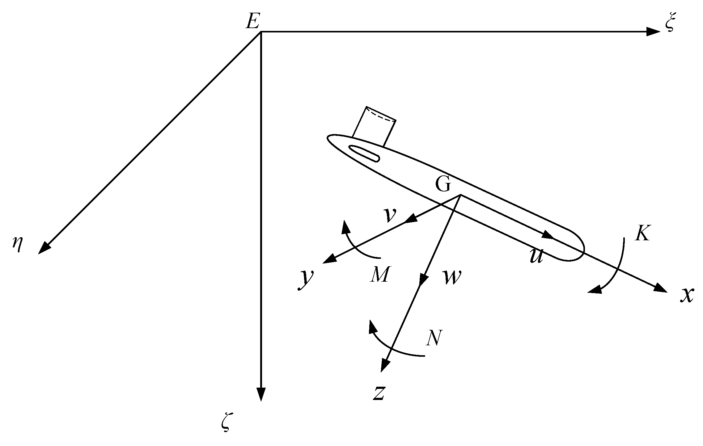
The right-hand Cartesian coordinate system is shown in Figure 1. One is the geodetic coordinate system E-ξηζ, referred to as the “fixed system”, which is fixed to the earth. The other is the body coordinate system G-xyz, referred to as the “motion system”, which is moving with the underwater robot.
The space position of the underwater robot can be determined by the coordinate of the motion system relative to the fixed system and three attitude angles of the motion system relative to the fixed system, that is, . The state information can be expressed by the velocity and angular velocity of the underwater vehicle under the motion system, that is, , the force and torque provided by the actuator of the underwater robot are expressed as . The velocity, angular velocity, force, and torque of the underwater robot are expressed by the parameters in Table 1.
2.2. The Mathematical Model Used in This Paper
When AUV performs tasks, the environment is complicated and there are many static obstacles. In this paper, the mathematical model of obstacles in the Marine environment is:
where is the number of obstacles, represents the central coordinate of the obstacle, is the terrain parameter, controls the height of obstacles, and respectively are the attenuation amount and control slope of the obstacle along the -axis and -axis, is the height of the terrain expressed as the absolute position .
Ocean currents are an important factor that needs to be considered in the environment when AUV performs tasks. Reasonable use of ocean currents can reduce the difficulty of AUV operation, reduce navigation energy consumption and extend the service life of AUV. The mathematical model of ocean current is:
where is the map’s maximum depth, , , respectively are the velocity of the current along the direction of , , ; the strength of the current decreases with increasing depth.
Due to the existence of ocean currents, the actual sailing speed is different from the speed under the motion system. It is necessary to synthesize ocean current velocity and AUV velocity, and the mathematical formula is:
where is the resultant velocity vector of AUV in the case of ocean current, is the velocity vector of AUV, and is the velocity vector of ocean current.
AUV will encounter longitudinal resistance from the ocean currents during navigation, and the energy consumption of navigation mostly comes from overcoming the resistance energy consumption of navigation. The mathematical model of longitudinal resistance and pitch angle is:
where is the longitudinal resistance, and is the longitudinal inclination of AUV. It is assumed that is a constant value during AUV motion, so AUV longitudinal thrust .
In the path planning process of AUV, there are still some shortcomings in the way of considering the path length and energy consumption constraints. In order to ensure that the planned path is a smooth and feasible path, it is necessary to consider the mobility constraints of AUV in the planning process; a smooth feasible path can save energy and improve the efficiency of the control system. The mobility constraint model is:
where is the radius of curvature of the path point, is the minimum radius of rotation of AUV, is the angle between the path point and the horizontal plane, that is, it represents the inclination angle of AUV under ideal conditions; and are the minimum and maximum of the safe inclination angle of AUV.
3. Improved Particle Swarm Optimization Algorithm Based on Multiple Constraints
3.1. Mathematical Model of AUV Path Planning Problem
Normally, AUV path planning has three objectives: (1) to move the AUV from the starting point to the target point; (2) to make the planned path satisfy the requirements of AUV motion security; (3) to find the shortest path in the path planning.
However, for the study of this paper, in addition to the above two objectives, the following two objectives need to be satisfied: (1) to optimize the AUV path and plan a more energy-saving path; (2) to plan the path more in line with the mobility requirements of AUV. Therefore, the AUV path planning problem can be transformed into the optimization problem.
where is the number of path points, is the comprehensive cost function, that is, the optimization function of the planning problem, , , , is the weight of each constraint cost function , , , , respectively.
3.1.1. Path Cost Function
Although this paper aims to study the energy-saving path planning problem of AUV that satisfies the mobility constrain, the length of the path should be considered. In a complex environment, reducing the task path length of AUV will also increase the security of AUV task execution, so the path cost function of this paper is:
where is the length of the path of segment j.
The updating principle of path cost weight is:
where is the initial value of the weight of the path cost, is the vibration coefficient, and is the maximum updating range of . If is larger than , will also be larger, which means that the attention to path length in the iteration is increased.
3.1.2. Energy Cost Function
The energy consumption cost function considered in this paper is:
where is mainly composed of two parts, one is the energy consumption of the propeller , and the other is energy consumption caused by the angle between AUV and ocean current direction, as shown in Equations (10) and (11):
Among them, is the angle between the velocity direction of AUV and the velocity direction of ocean current. alone is not enough to represent the energy consumption of AUV sailing. Most AUV are not equipped with a side propeller, so when the AUV is perpendicular to the direction of the ocean current, it will affect the maneuverability of the AUV and consume more energy. With the existence of , the tangent of the planned route will be as low as possible perpendicular to the current direction, which is of great significance to reduce the energy consumption of AUV and improve its maneuverability.
The updating principle of energy cost weight is:
where is the default weight value, is the maximum weight update range.
3.1.3. Mobility Cost Function
The mobility cost function considered in this paper is:
where and are the initial value of weight, and are the maximum update range of the weight, represents the radius of path points that do not satisfy the minimum turning radius of AUV, and are the inclination angles of path points that do not satisfy the constraint of inclination angles, and represent the radius of gyration and trim angle cost function, which means to describe the unsatisfied degree of path points and maneuverability constraints. The way to update the weight is to increase the degree of attention in the comprehensive function when the degree of dissatisfaction increases, that is, to give a punishment mechanism to this behavior, and to optimize the path in the direction of satisfying the mobility constraint.
To sum up, the particle swarm fitness function is set as the comprehensive cost function .
3.2. Particle Swarm Renewal Law
3.2.1. Particle Swarm Velocity Renewal Law
In this paper, the speed updating method of traditional particle swarm optimization is improved, and the improved method is:
where is the inertia weight, representing the degree of trust in the current speed direction, and respectively represent the learning efficiency in the individual and in the whole particle, , , are the random values between , increase the search randomness, represents the degree of trust in the speed jump, represents the speed of the particle in the generation, represents the position, and respectively represent the individual optimal fitness and global optimal fitness, is the number of the same global fitness in each generation, and is the maximum number of the same global fitness. The detailed meaning is that when the global fitness in each generation increases for the same number of times, the randomness is increased so that the particle has a chance to jump out of the local optimal solution.
The velocity of each particle must be between the minimum particle velocity and the maximum particle velocity .
As for the prematurity of traditional particle swarm optimization algorithms, , , and are updated according to the nonlinear processing mode, and the detailed formula is:
where is the current iteration number, is the maximum iteration number, , and are respectively the attenuation proportional coefficient of particle’s local learning efficiency, the attenuation proportional coefficient of particle’s global learning efficiency, and the attenuation coefficient of particle’s trust in speed jump. The compression factor is used to update the inertia weight . In this way, different regions can be searched effectively, high-quality solutions can be obtained, and the convergence speed of the algorithm can be appropriately increased. is the minimum value that speed jump weight can reach, and are the maximum value that learning efficiency can reach. In this paper, it is hoped that the inertia weight decreases gradually with the increase in iteration times, while increases gradually to increase the local searchability. At the same time, will decrease with the increase in the number of iterations, which means that with the learning of each generation of particles, particles will be more confident in the judgment of individuals and populations, the random jump of speed will be weakened, and particles will become more intelligent.
3.2.2. Particle Swarm Initialization Renewal Law
When , it is considered to be trapped in the local optimal solution, and the population needs to be re-initialized. If the population is randomly initialized, the convergence speed of the algorithm will be slowed down. Therefore, the initialization population rule is:
where is the standardized function. By standardizing the solution set trapped in the local optimal solution and combining it with the local optimal solution, a new solution set is obtained, which increases the probability of the particle jumping out of the local optimal solution without deviating too far from the high-quality solution set and reduces randomness. At the same time, these locally optimal solutions are packaged in a feasible solution set, because the most suitable solution is most likely to be in this solution set. Finally, the feasible solution set is compared with the global optimal fitness, and the smaller one is the optimal solution of the EPA-PSO algorithm.
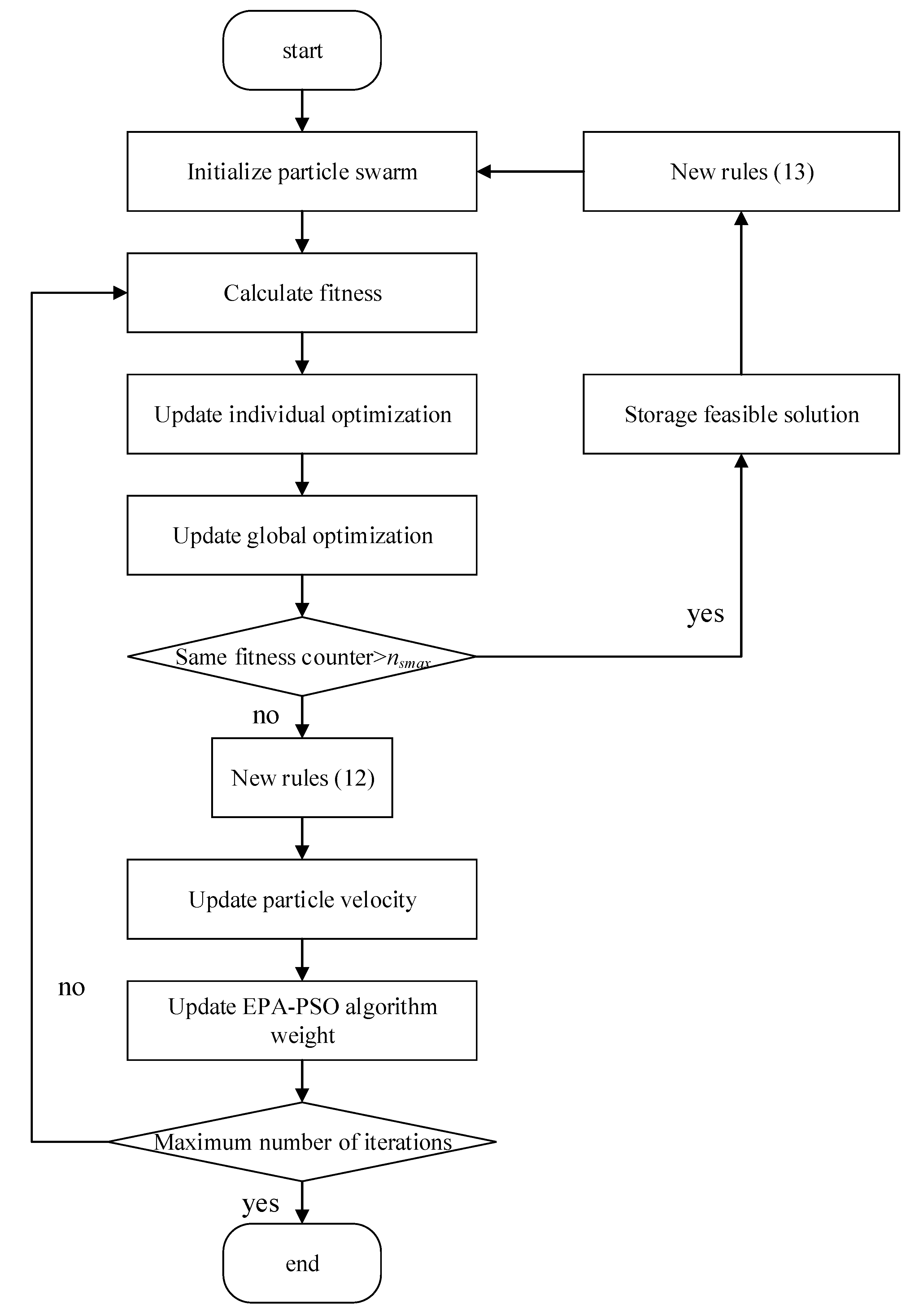
After the above algorithm is improved, the flow of the algorithm is shown in Figure 2:
4. The Simulation Results
At first, it is convenient for the experiment to proceed smoothly; this paper makes some assumptions about the path planning of AUV: (1) AUV is considered as a particle, and the external size of AUV is ignored. (2) The thrust of the AUV is equal to the resistance during navigation, and the resistance is only related to the inclination of the AUV. (3) In the ocean current environment, the AUV velocity is strictly parallel to the tangent line of the planned path.
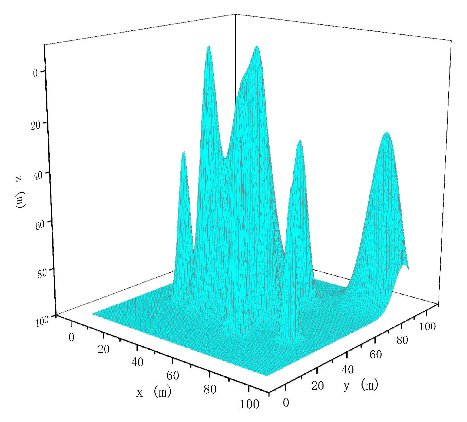
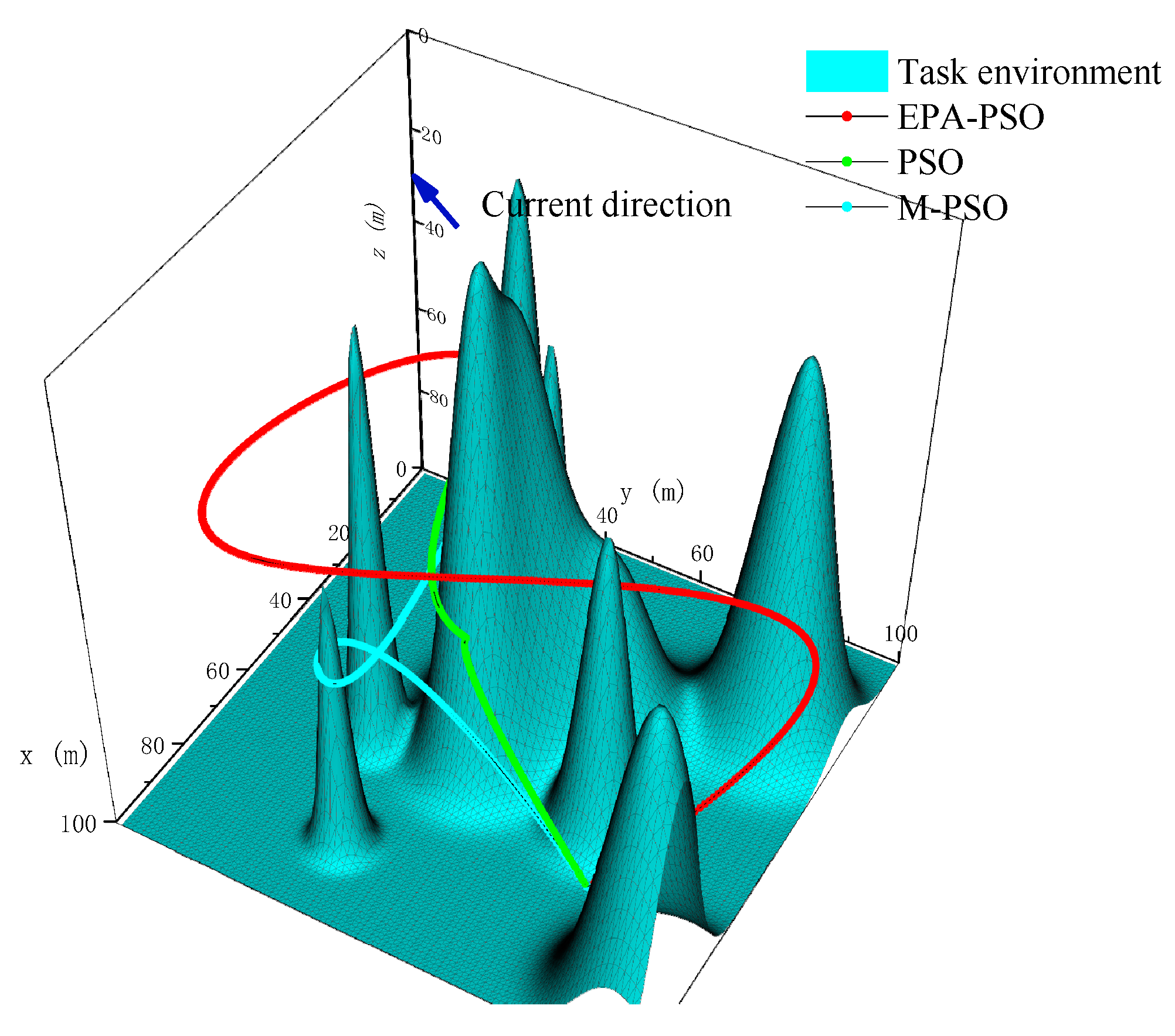
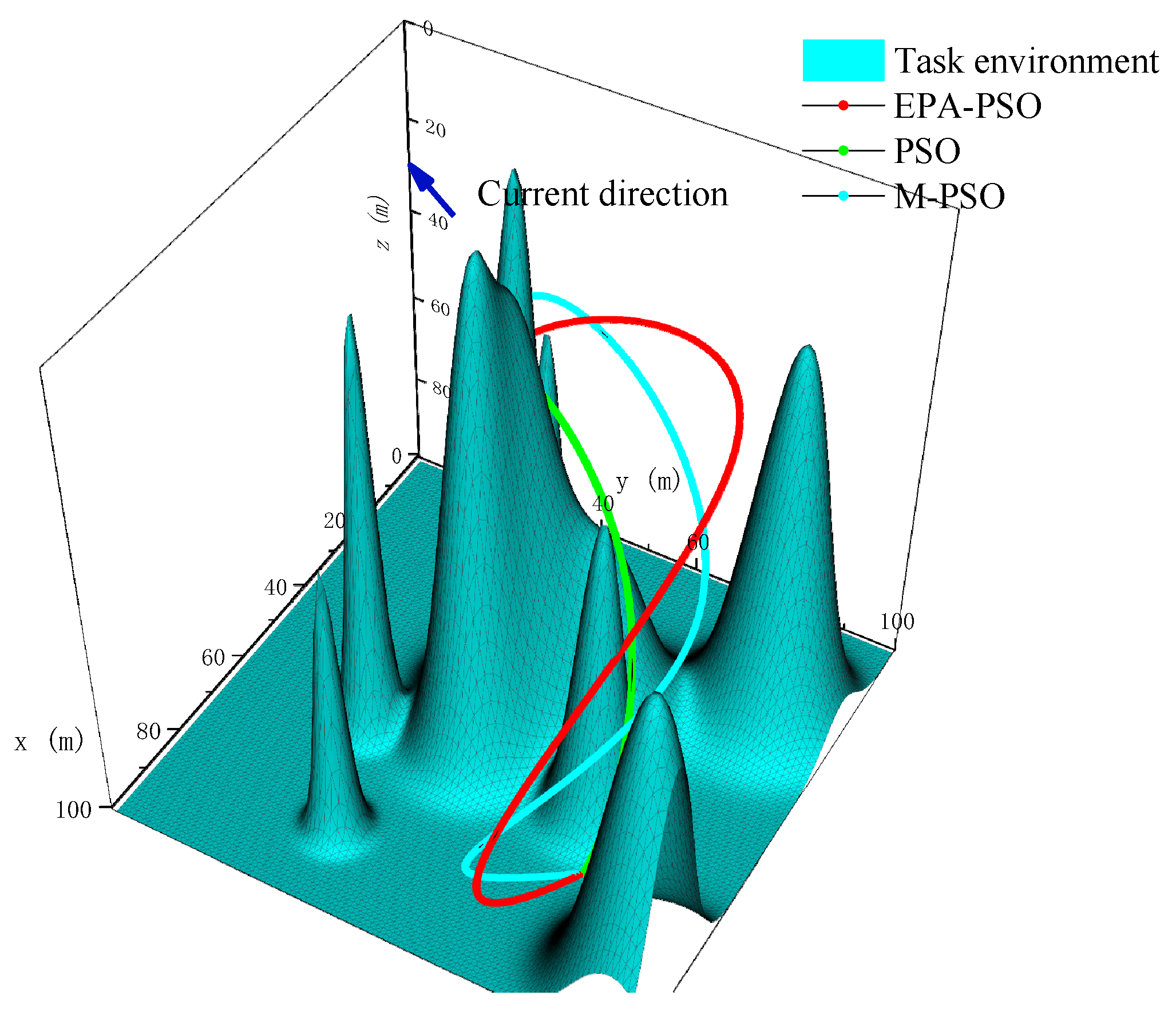
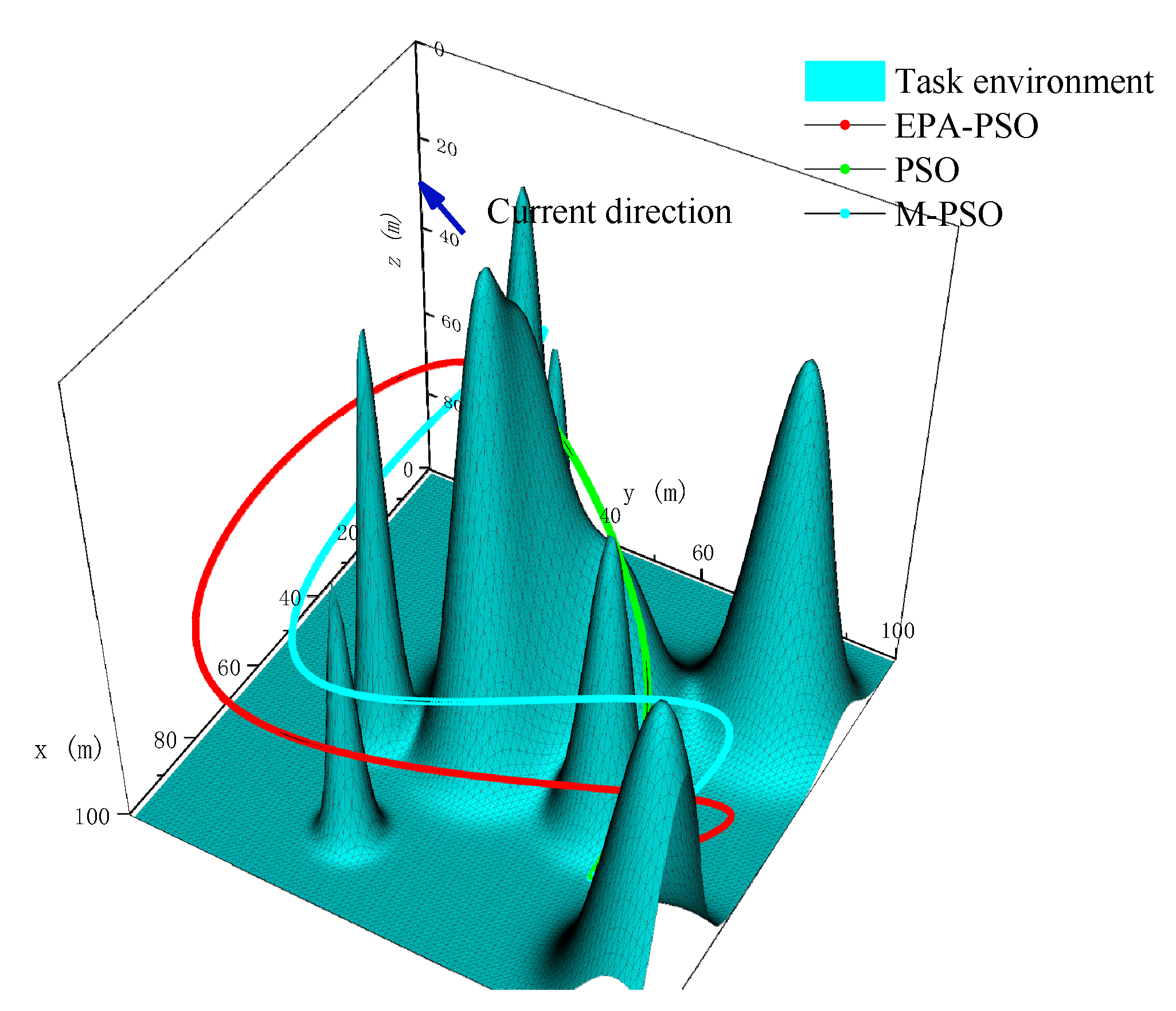
The task environment of AUV is shown in Figure 3, and the number of obstacles is 10.
Some parameters of the improved algorithm in this paper are shown in Table 2, where is the number of particles.
The starting point of AUV is set to , the finish point , comparing the PSO algorithm considering only the path length with the PSO algorithm considering constraints (temporarily named M-PSO algorithm) and the EPA-PSO algorithm proposed in this paper, the AUV path planning simulation experiment is conducted. Iteration times are set to 100, 200, 500 respectively. At the same time, since the units of each cost function are inconsistent, normalization is carried out for them, and the simulation results are finally obtained as shown in Figure 4, Figure 5, Figure 6, Figure 7, Figure 8, Figure 9, Figure 10, Figure 11, Figure 12, Figure 13, Figure 14, Figure 15, Figure 16, Figure 17, Figure 18, Figure 19, Figure 20, Figure 21, Figure 22, Figure 23 and Figure 24:
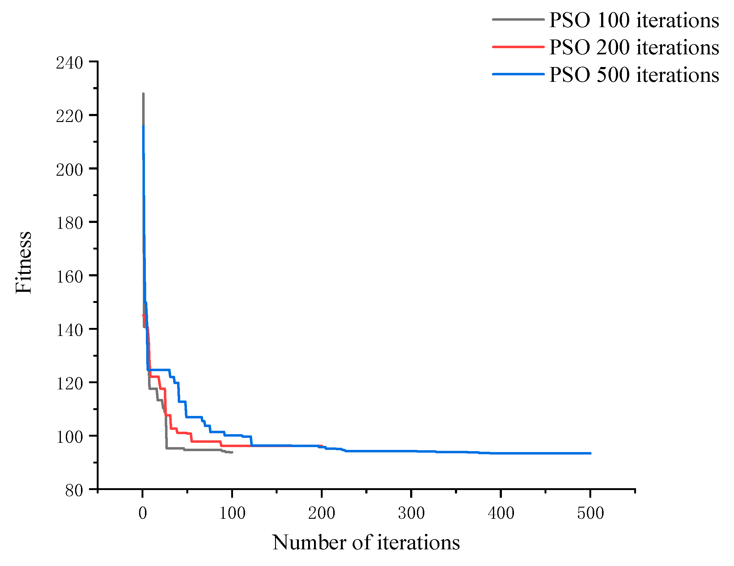
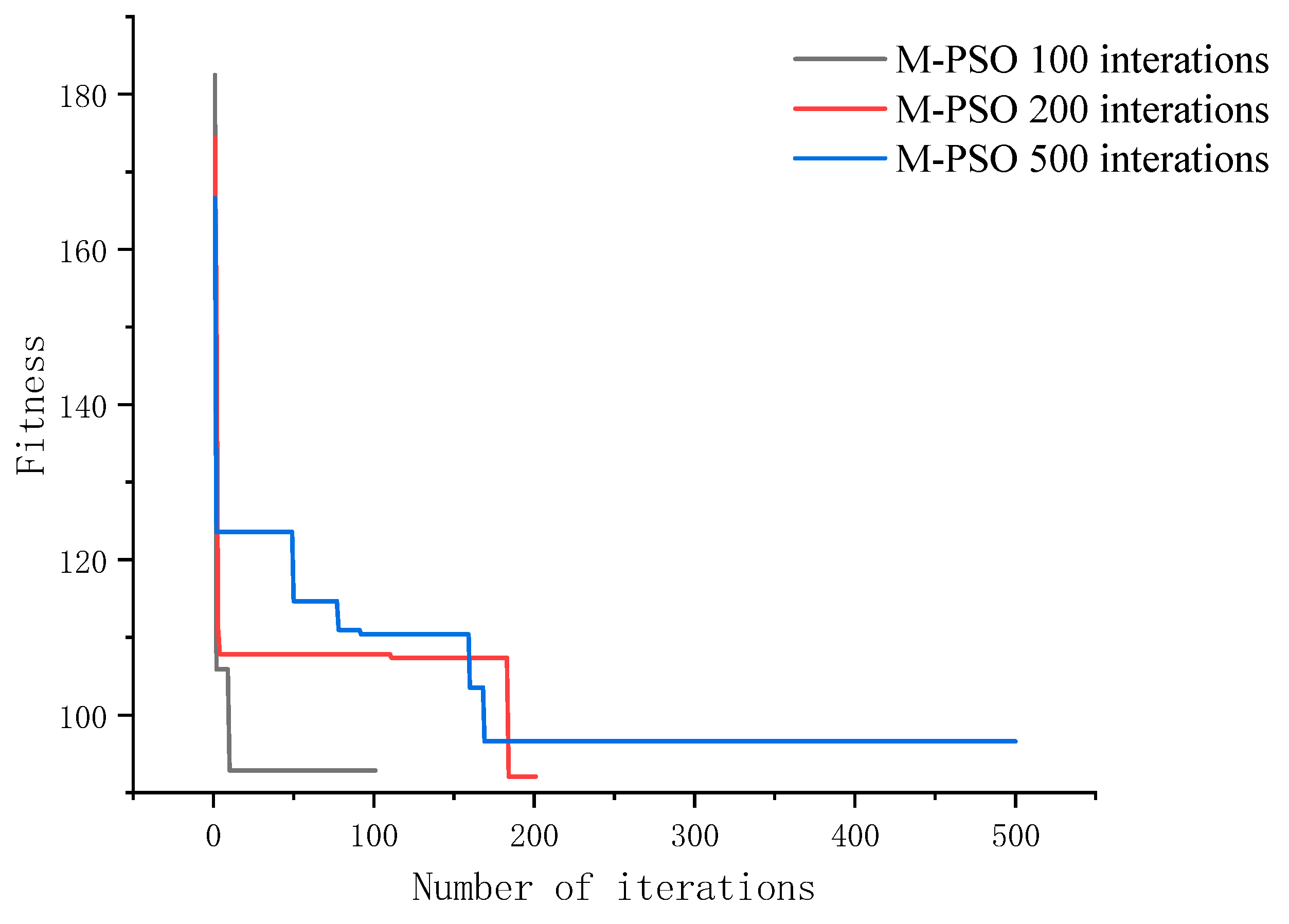
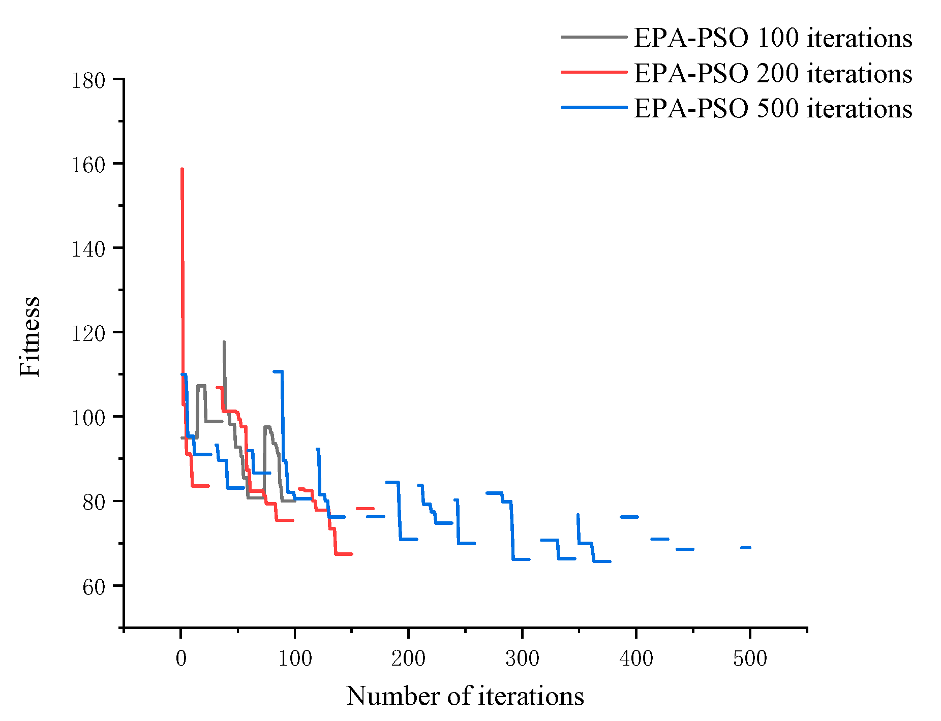
Figure 4 shows that with the increase in iteration times with the traditional PSO algorithm, the problem of constant fitness of traditional PSO algorithm has become more and more prominent, which will lead to too many instances of staying on a solution that satisfies the constraint and wastes too much time. M-PSO has the same problem, the algorithm will be too precocious, the fitness will not change much for the later iteration. It can be seen in Figure 6 that although the convergence speed of the EPA-PSO algorithm proposed in this paper is slower, it can solve the premature problem of the traditional PSO algorithm, enhance the random searchability of the traditional algorithm, and make it more likely to find the optimal solution in line with constraints.
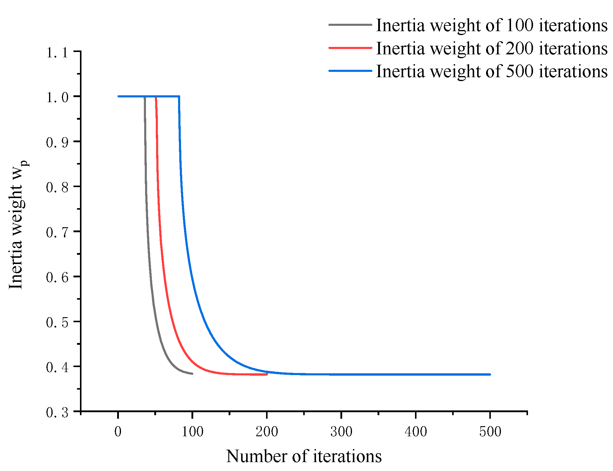
Inertia weight adjustment strategy as shown in Figure 7 shows the rate of its adjustment is not static, but gradually decreases with the increase in algebra. When the algebra is small, the update rate is relatively slow, which makes the algorithm have a good global searchability. With the increase in algebra, it gradually decreases, thus enhancing the local searchability.
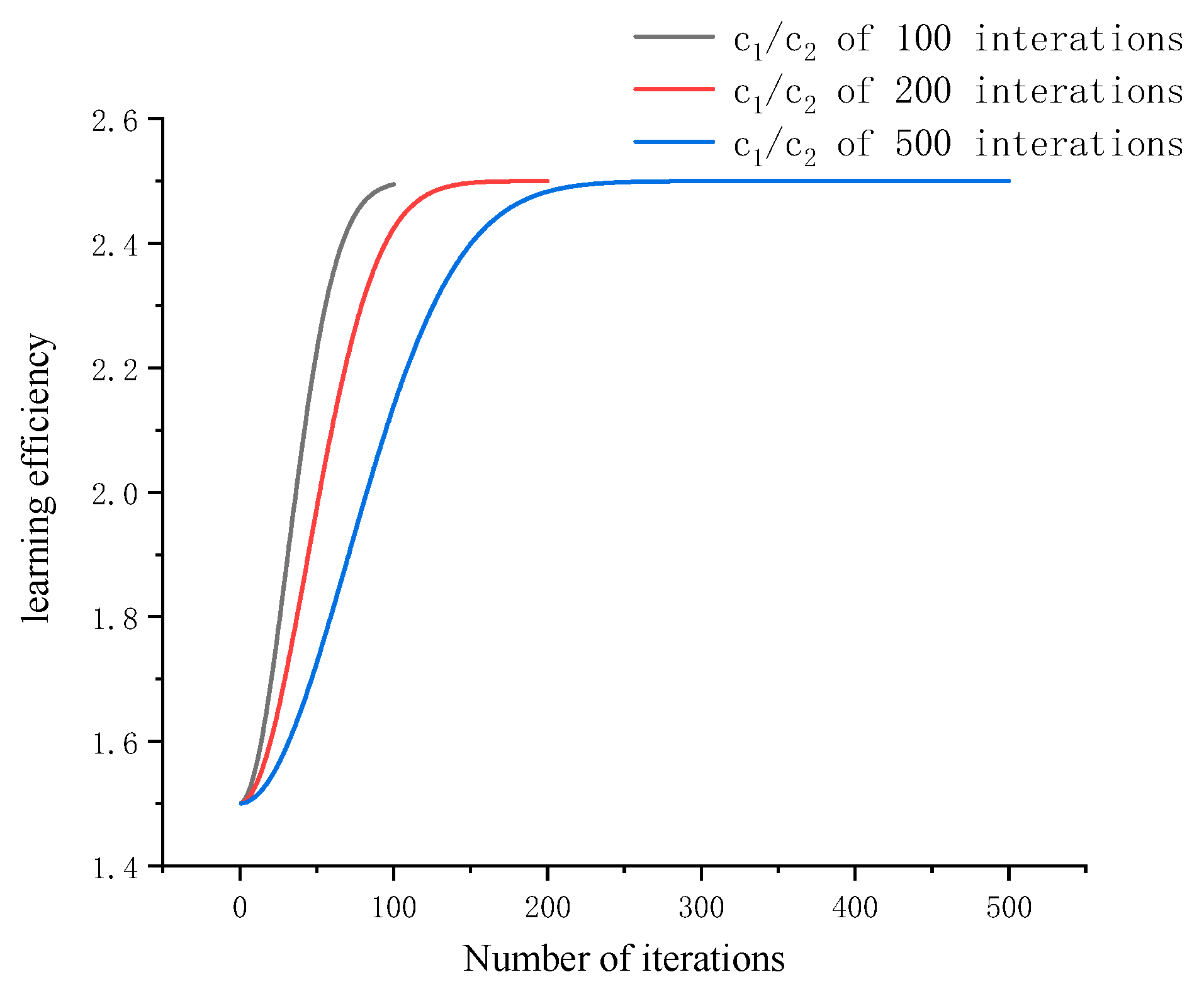
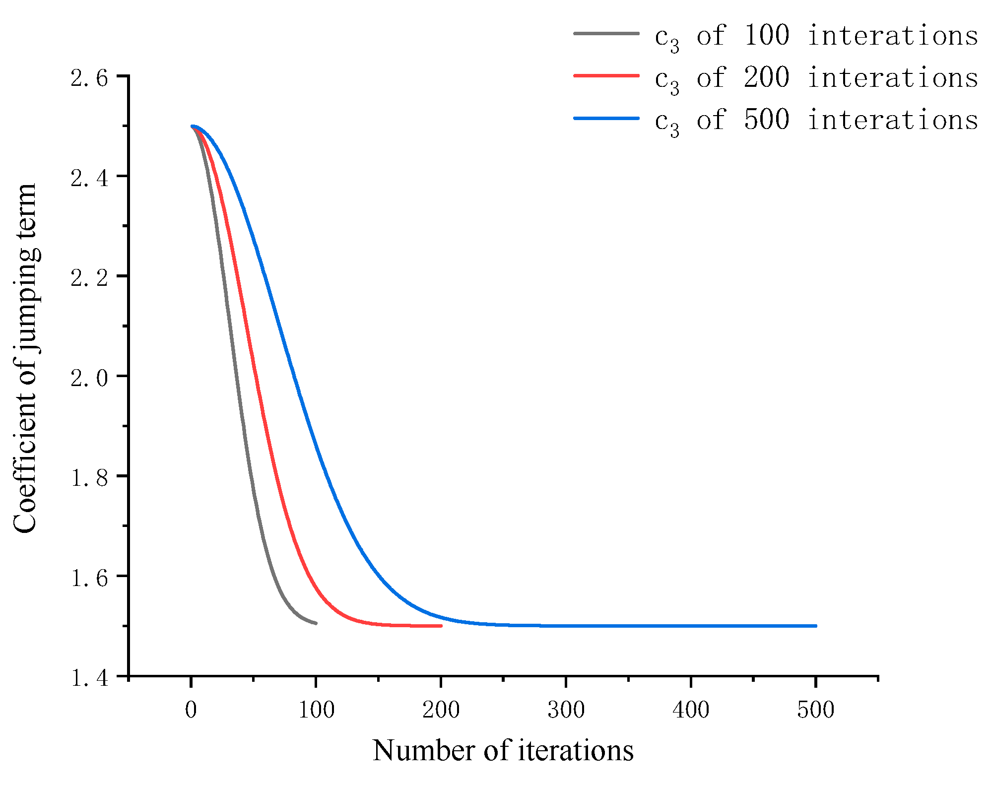
Figure 8 and Figure 9 are , , respectively. With the number of iterations increasing, and first increase slowly, then increase rapidly, and finally tend to be stable, which makes it have a better global search ability at the initial stage of iteration, and then enhances its local search ability. With the increase in iteration times, will gradually become smaller, which means that particles are more and more trusting in the judgment of individuals and populations in the process of evolution, and will reduce the probability of speed jump.
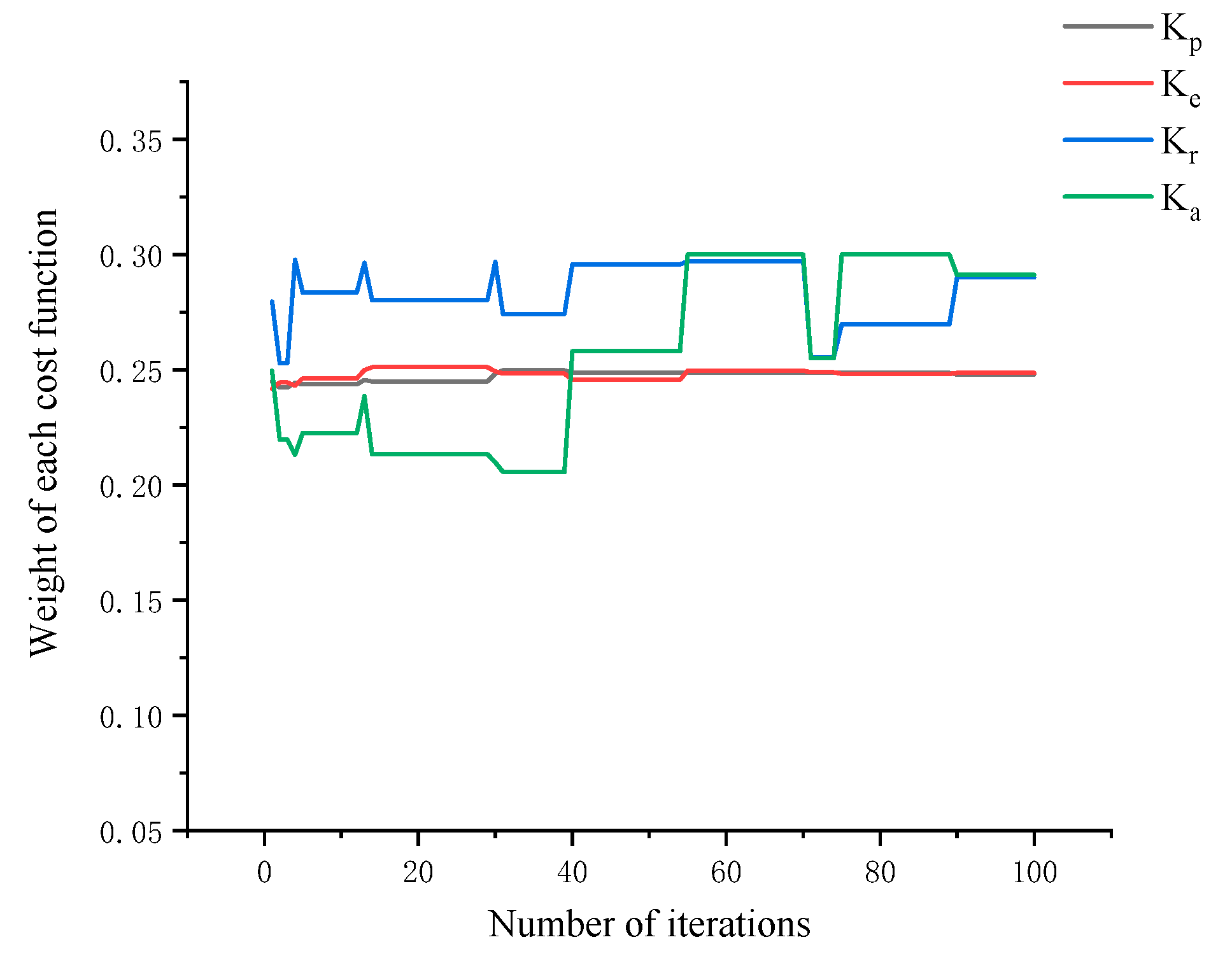
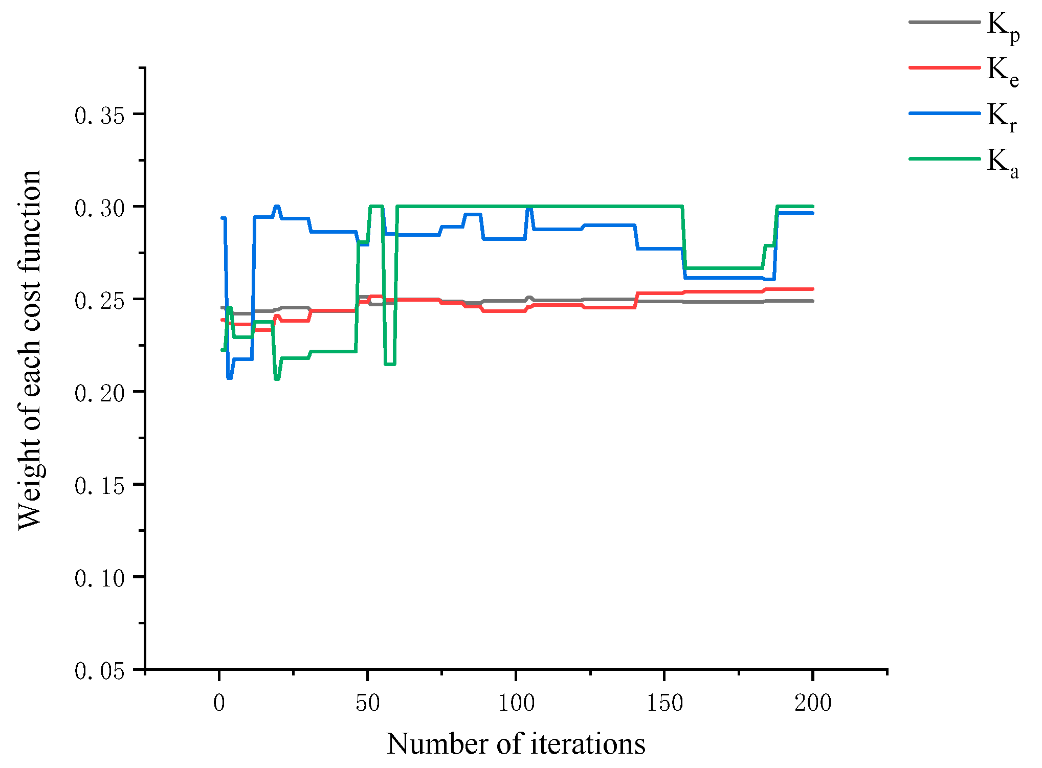
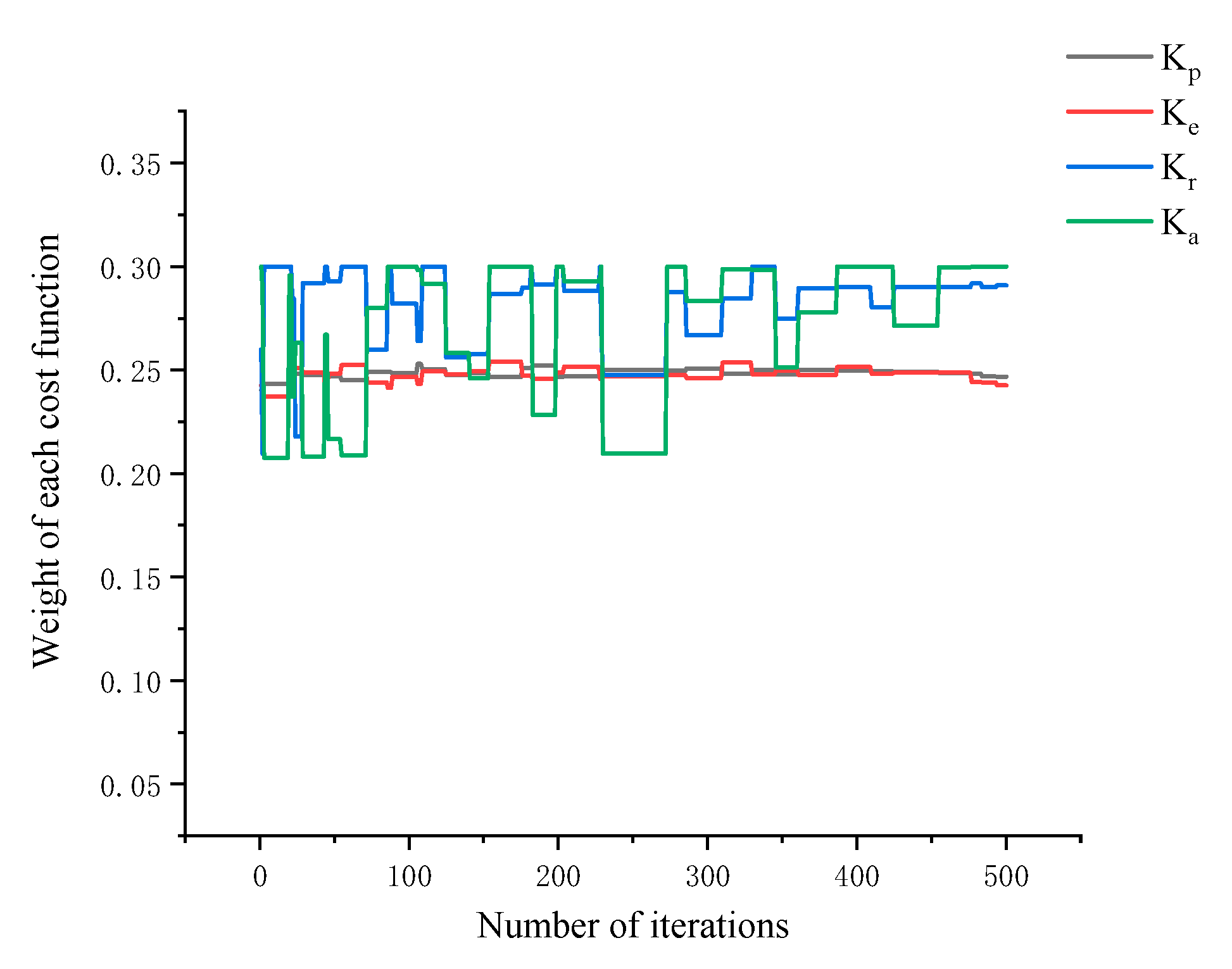
Figure 10, Figure 11 and Figure 12 can reflect that the weight of each cost function can be dynamically adjusted during the implementation of the algorithm, that is, the reward and punishment mechanism of the cost function takes effect and makes the algorithm run in the direction of the optimal solution more effectively.
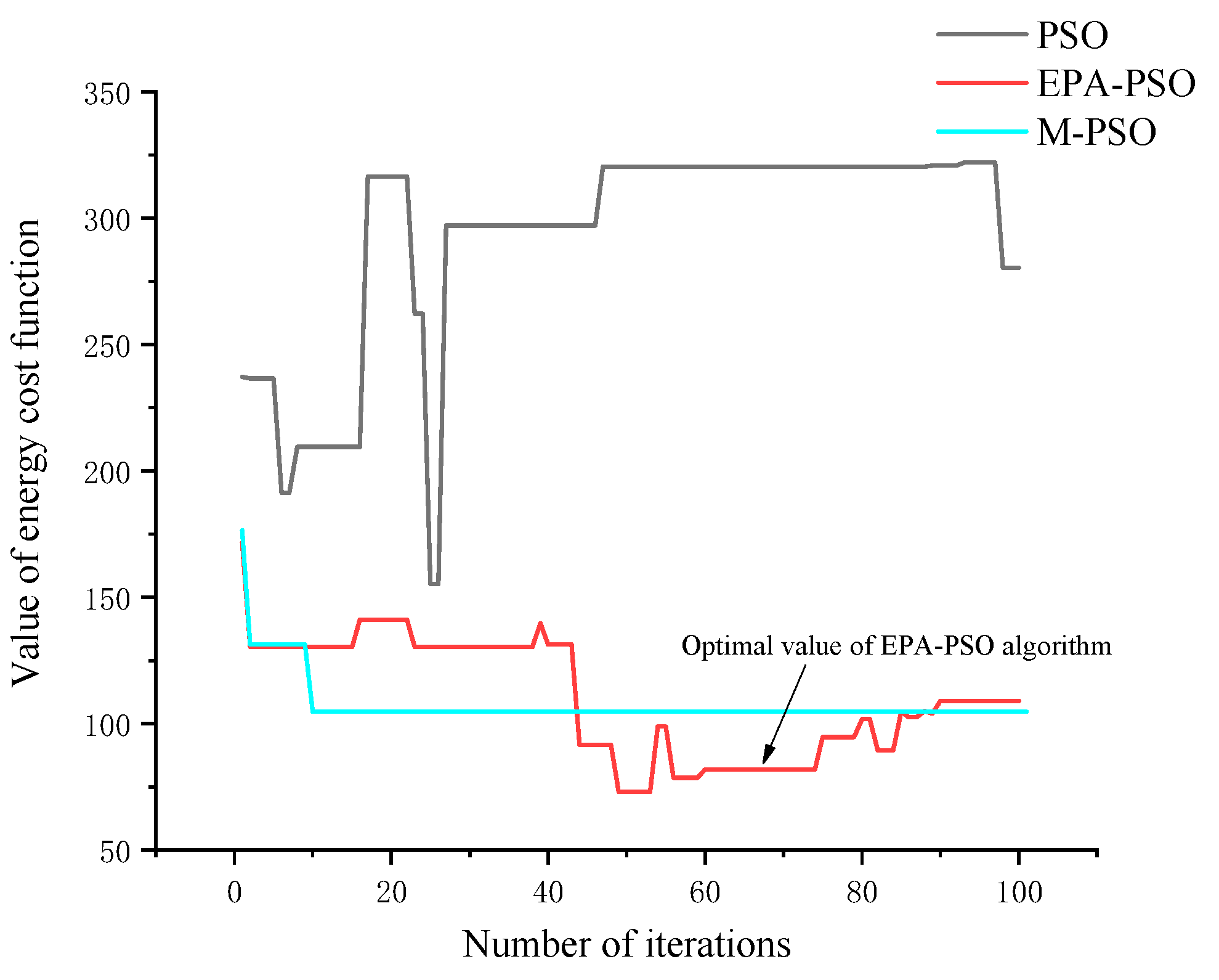
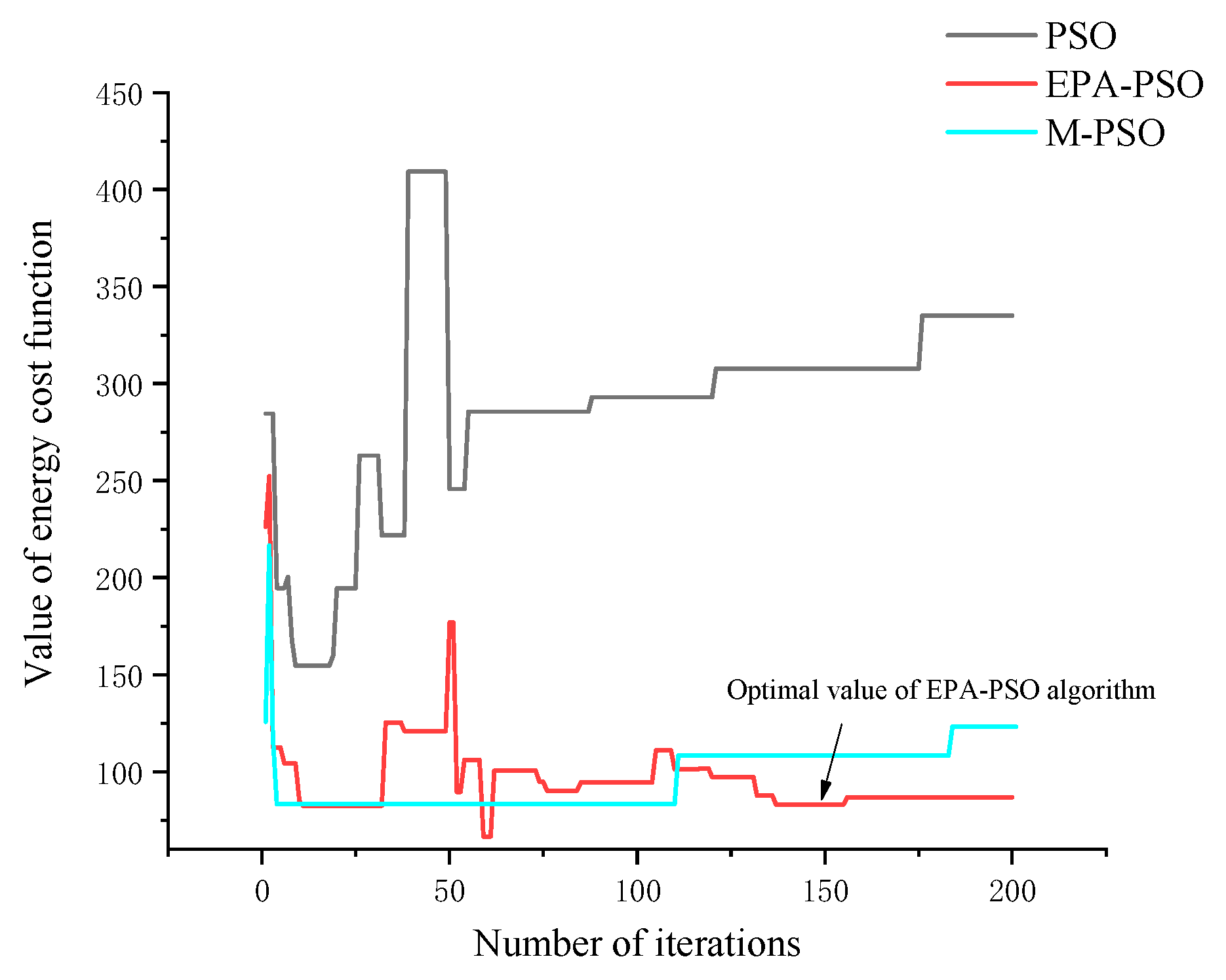
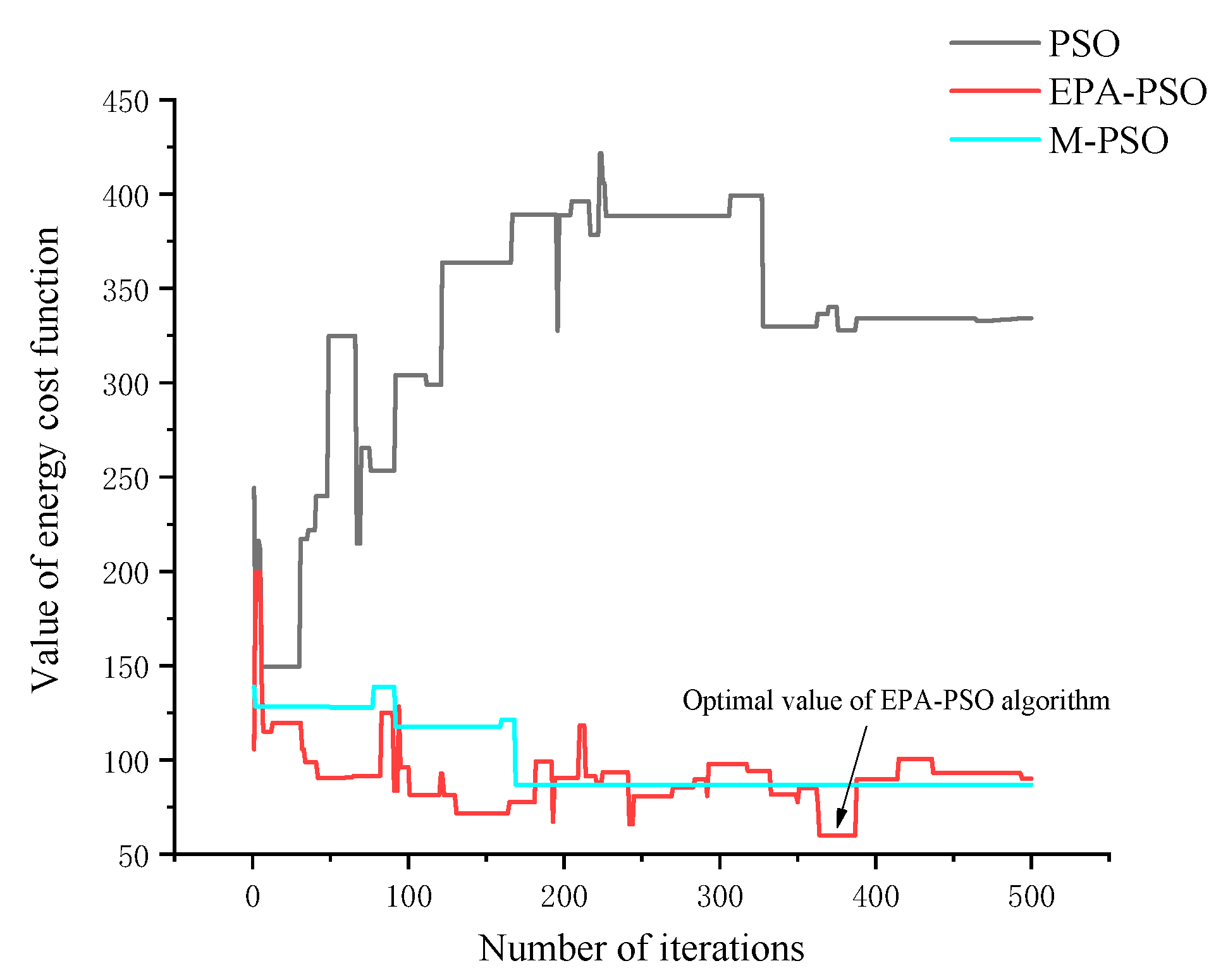
According to the energy consumption comparison test in Figure 13, Figure 14 and Figure 15, both M-PSO and EPA-PSO can significantly reduce the energy consumption in the planning process. Compared with the traditional PSO algorithm, M-PSO has 100 iterations and 200 iterations respectively. The energy efficiency of 500 iterations reached 66.67%, 63.21%, and 73.95%. At the same time, compared with M-PSO, EPA-PSO proposed in this paper is more effective in reducing energy consumption in AUV path planning, with energy rates reaching 70.81%, 75.18%, and 81.99% in 100 iterations, 200 iterations, and 500 iterations.
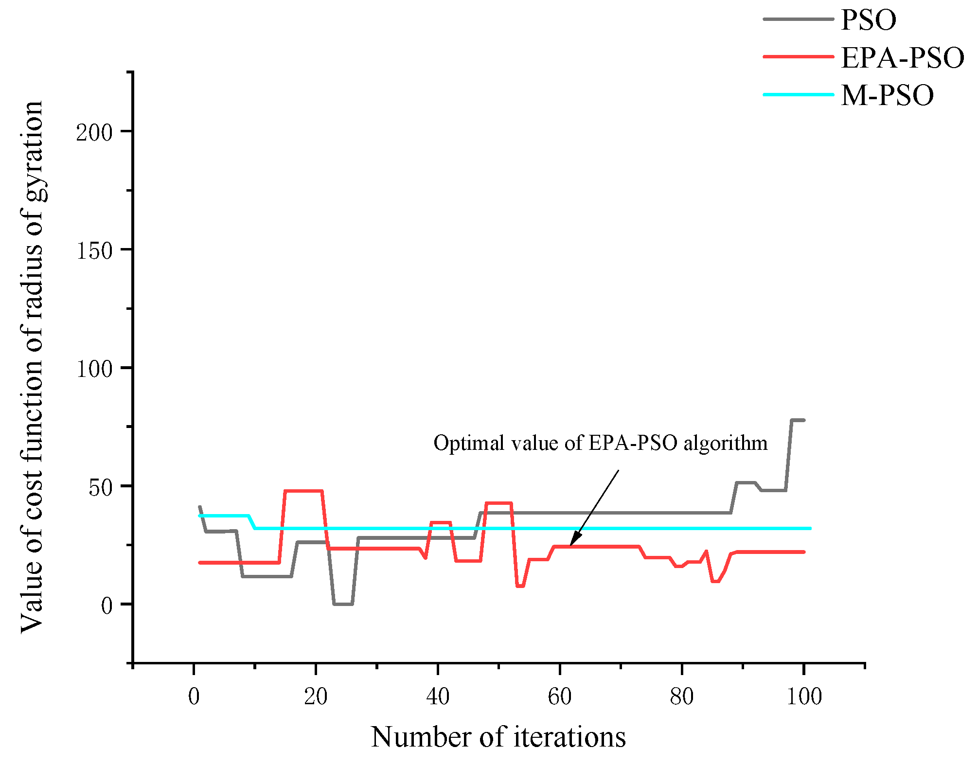
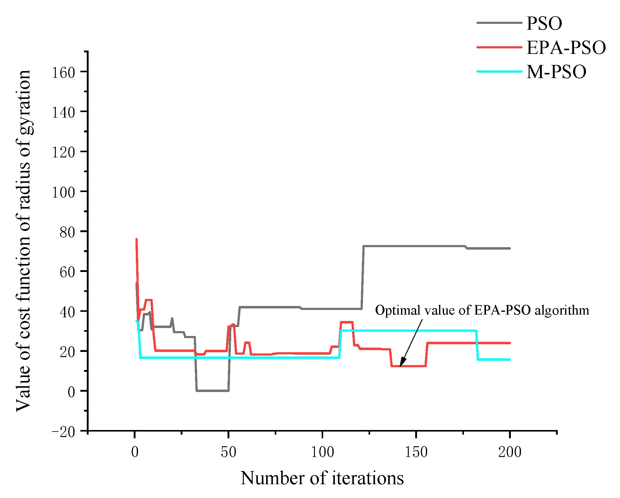
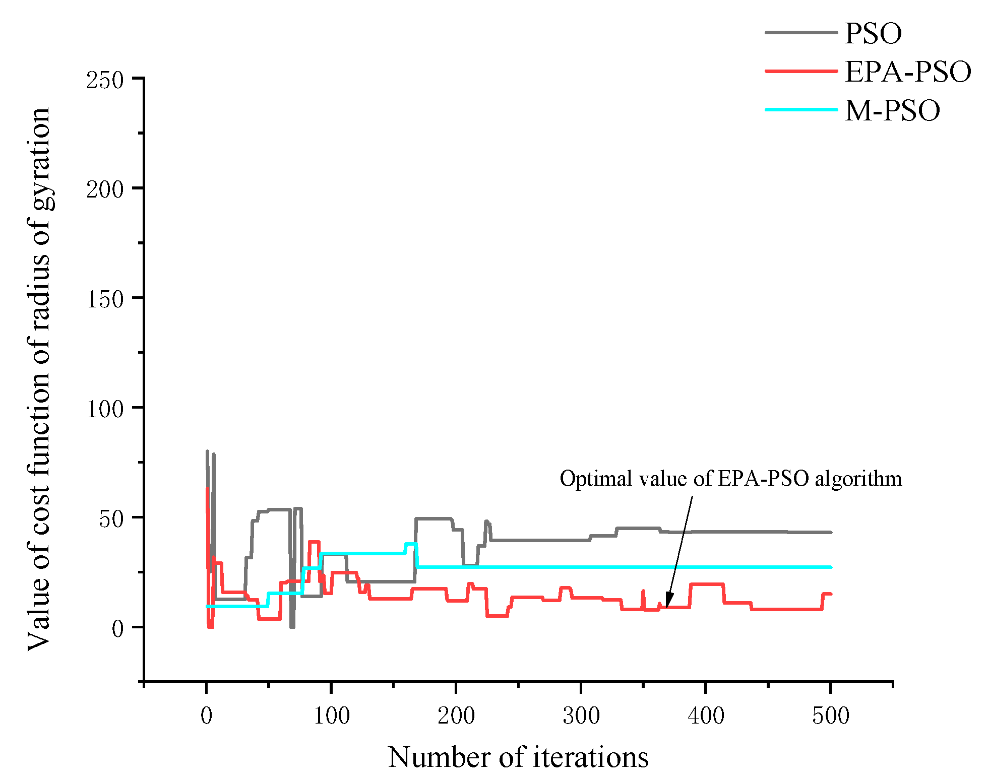
It can be seen from the comparison test of rotation performance in Figure 16, Figure 17 and Figure 18 that both M-PSO and EPA-PSO can significantly increase the feasibility of the AUV planning path. M-PSO is in 100 iterations, 200 iterations, and 500 iterations, the cost reduction rates of the radius of rotation are 58.80%, 78.05%, and 36.68%, and the results obtained by the EPA-PSO algorithm are better than those obtained by M-PSO algorithm. In 100 iterations, 200 iterations, and 500 iterations, the cost reduction rates of the radius of rotation are 68.78%, 82.64%, and 79.66%.
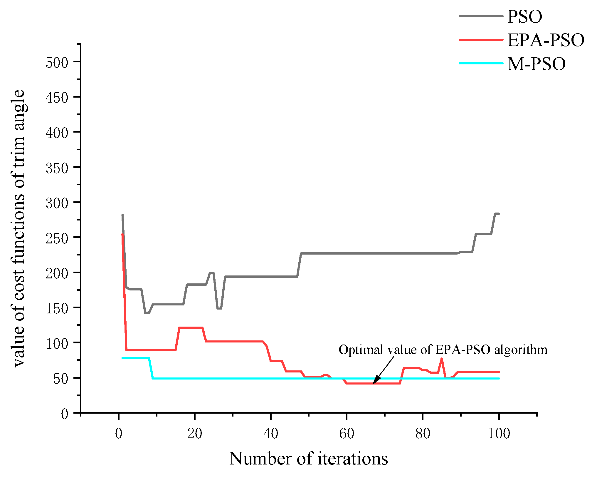
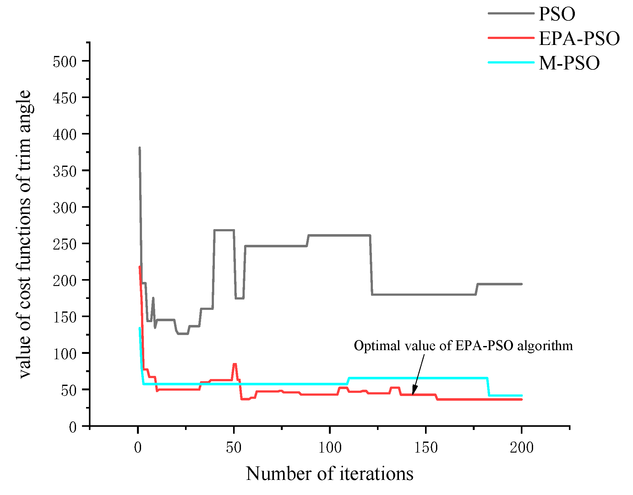
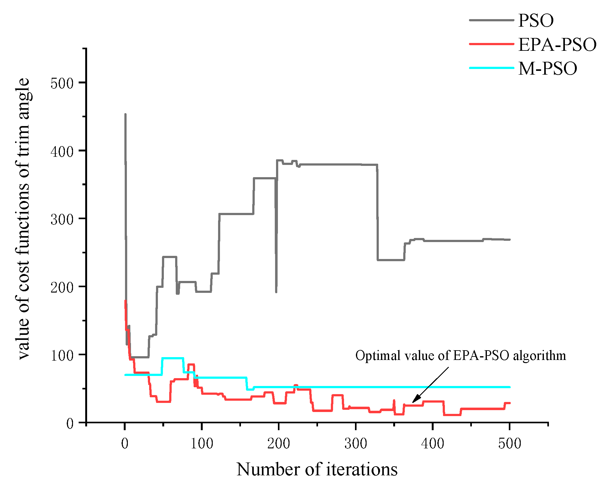
As can be seen from the longitudinal angle comparison test in Figure 19, Figure 20 and Figure 21, M-PSO and EPA-PSO can significantly reduce the degree of unsatisfied AUV safety trim angle in the planned AUV path. M-PSO is in 100 iterations, 200 iterations, and 500 iterations, the reduction rate of was 82.76%, 77.59%, and 80.65%. The EPA-PSO algorithm proposed in this paper is more effective than M-PSO, and the reduction rate is 85.28%, 77.98%, and 90.70% in 100 iterations, 200 iterations, and 500 iterations. As can be seen from Figure 22, Figure 23 and Figure 24, with the increase in iterations, the path length planned by the EPA-PSO algorithm is gradually getting longer; in other words, the increase in path length is necessary and reasonable in exchange for a path with lower energy consumption and better mobility of AUV
It can be seen in Table 3 that both M-PSO and EPA-PSO can reduce energy consumption in the process of AUV planning and make the path satisfy the requirements of AUV mobility. However, the overall effect of the EPA-PSO algorithm proposed in this paper is better. Meanwhile, compared with the experiment of M-PSO, it can be seen that simply changing the fitness function still leads to the problem that the PSO algorithm is easy to fall into the local optimal solution, resultingly the effect of 500 iterations is not as good as that of 200 iterations. Compared with the EPA-PSO algorithm proposed in this paper, better solutions can still be found as the number of iterations increases.
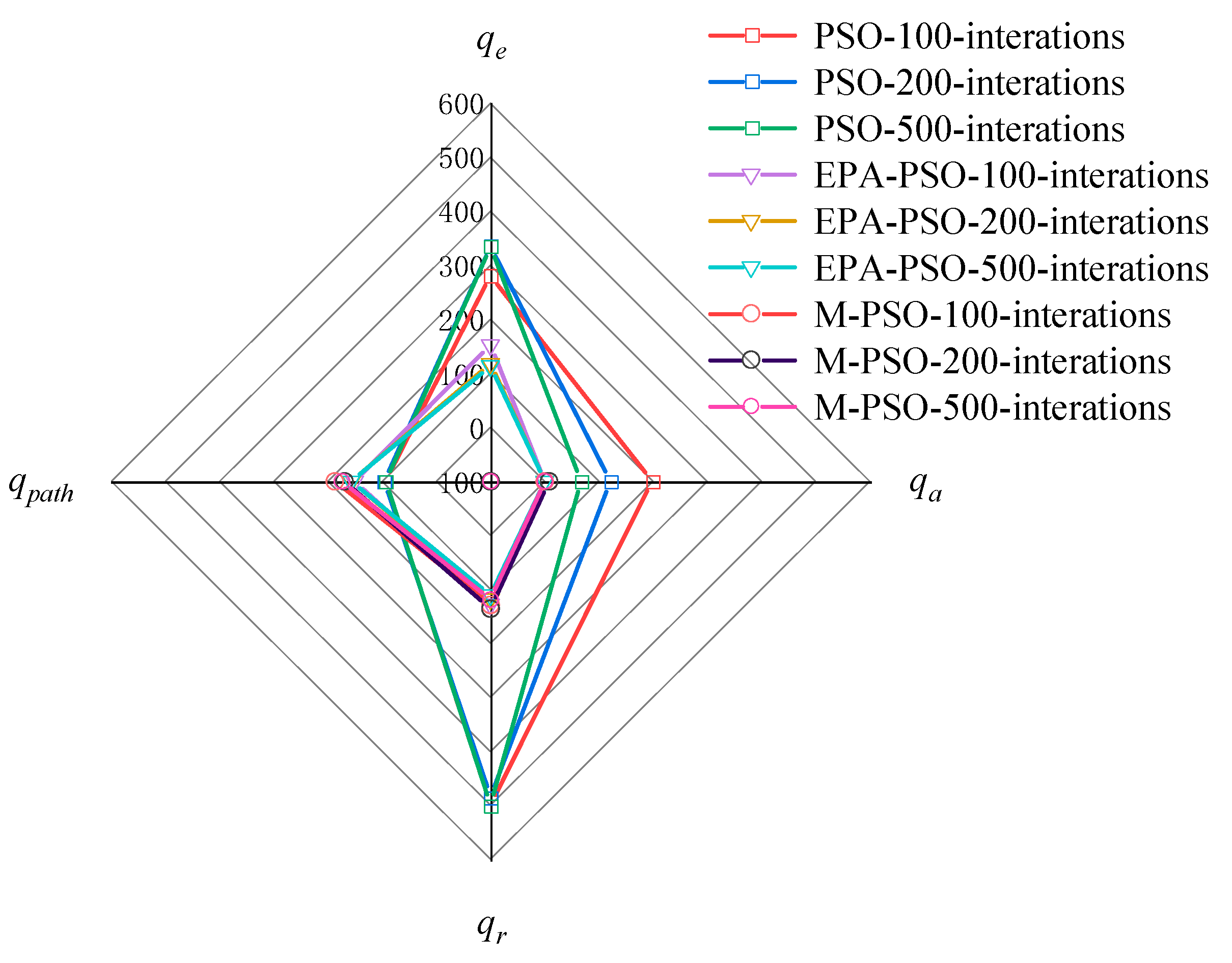
Therefore, EPA-PSO can solve the problem of the local optimal solution of the traditional PSO algorithm, but the weight of each cost function of the EPA-PSO algorithm is different, so it is necessary to use the evaluation criteria of Equation (18) and radar diagram to intuitively reflect the superiority of EPA-PSO algorithm in AUV path planning.
According to the new standard, it can be seen that the EPA-PSO algorithm proposed in this paper is more advantageous than the traditional PSO algorithm and M-PSO algorithm, and in the radar diagram the area enclosed by the EPA-PSO algorithm is the smallest in 500 iterations. Therefore, EPA-PSO proposed in this paper can solve the problem of AUV energy-saving path planning considering mobility constraints.
5. Field Test
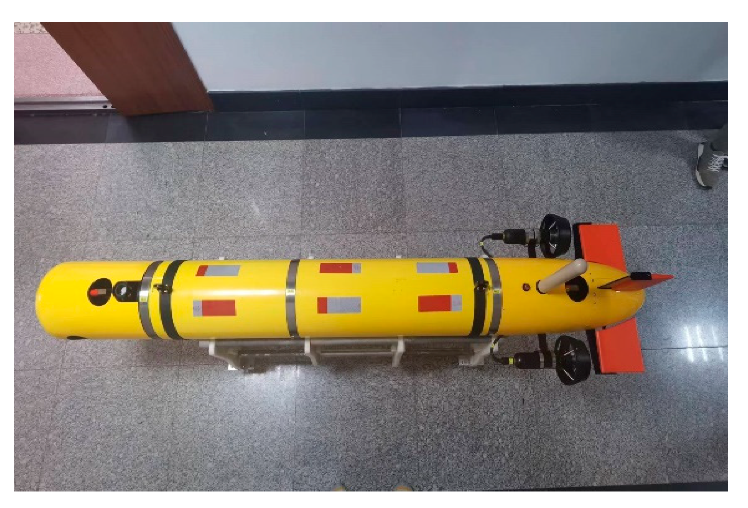
The feasibility of the EPA-PSO algorithm was verified in a series of offshore trials in Shanghai in February 2022. The validation platform was an AUV developed by Harbin Engineering University, which was mainly equipped with a tail propeller, cross rudder, side propeller, vertical propeller and other actuators. At the same time, it is equipped with sensors such as the Doppler Velocity Sonar (DVL), Magnetic Compass, altimeter, depth gauge, Inertial Navigation System (INS), the Beidou navigation system, and a radio communication system. According to relevant basic control experiments, the radius of rotation of AUV is about 5 m.
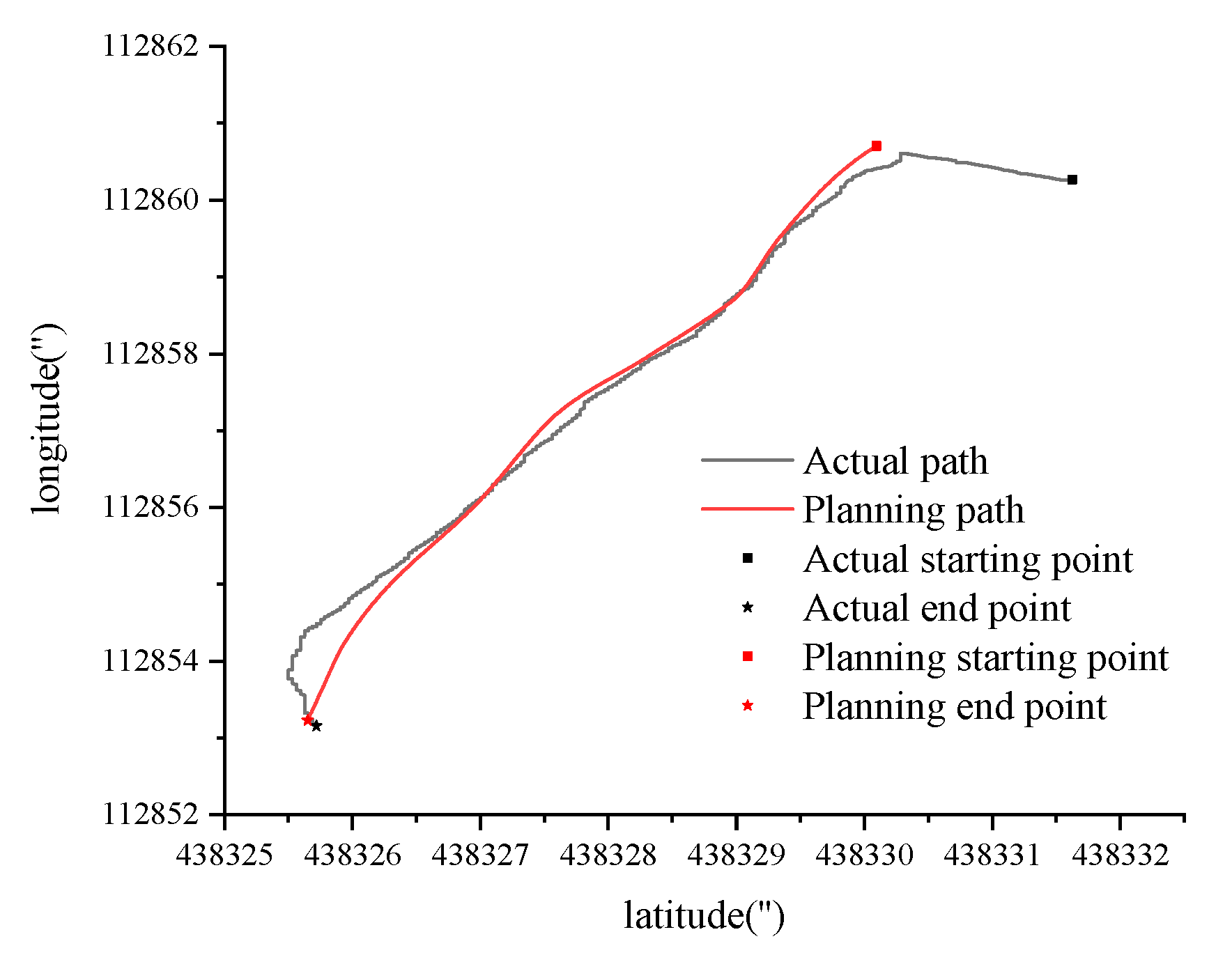
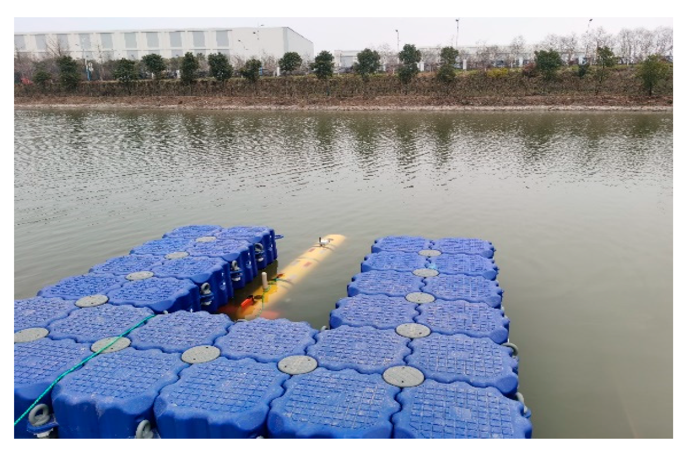
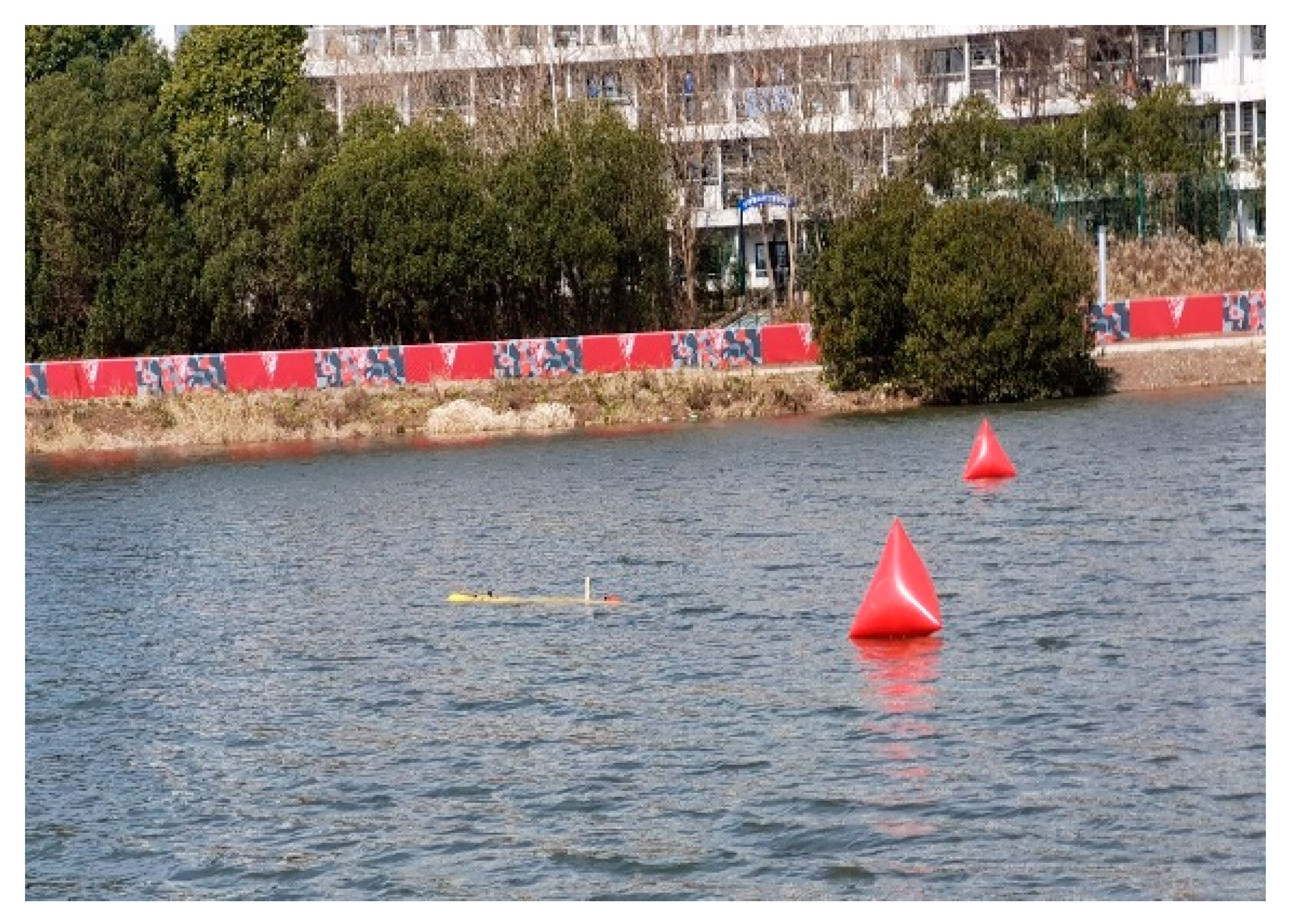
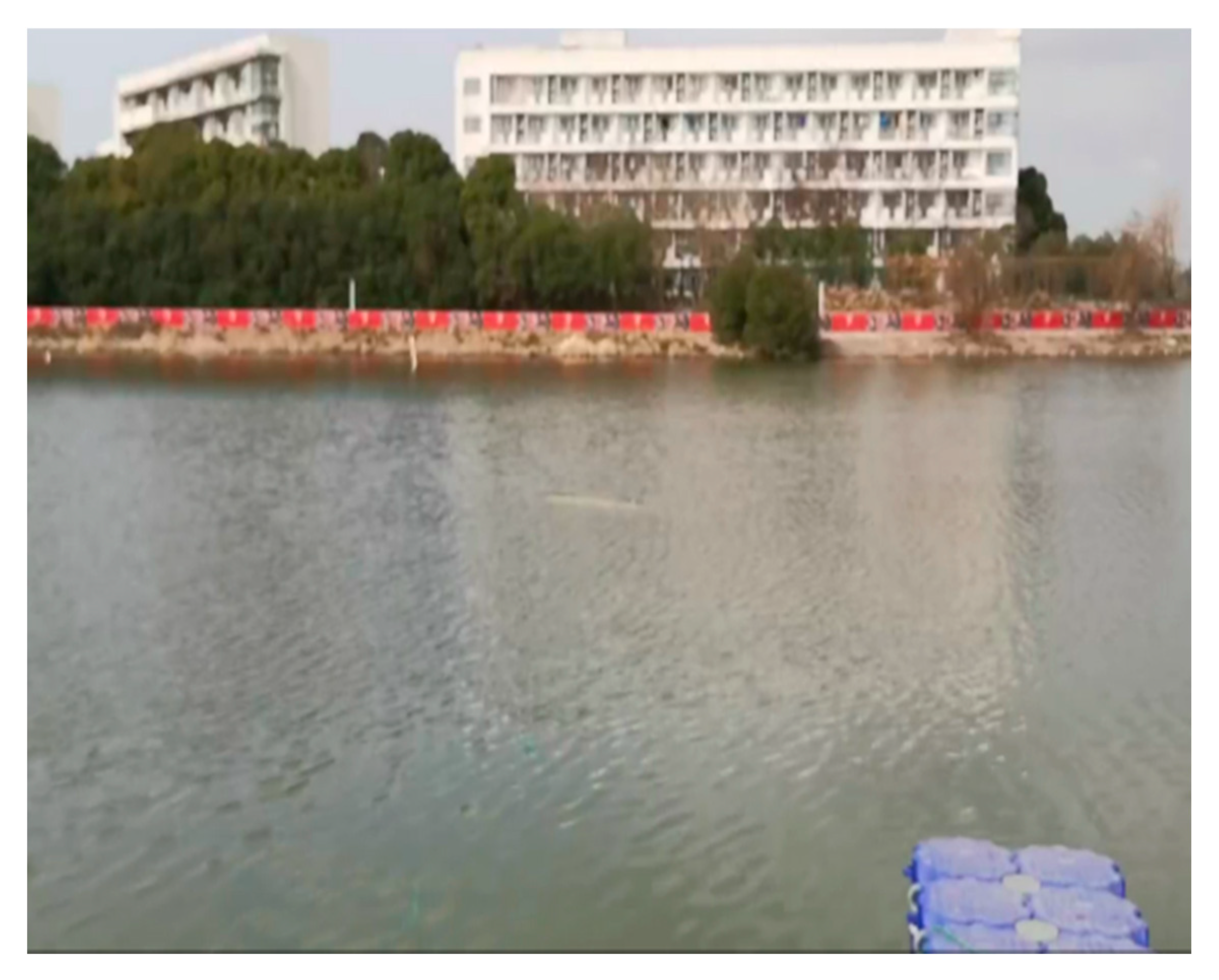
As shown in Figure 26, it is the experimental AUV used in the field test. Figure 27 shows the global planned route (red line in the figure) and the real AUV navigation route (black line in the figure) under the condition that obstacle information is known through the EPA-PSO algorithm proposed in this paper. The latitude and longitude of AUV are 438331.6250 s N and 112860.2660 s E, 438325.7190 s N and 112853.1560 s E. The longitude and latitude of the planned starting point and endpoint are 438330.0940 s N and 112860.2660 s E, 438325.6500 s N and 112853.2300 s E. As shown in Figure 28, it is the state that the AUV is ready to accept task instructions in the dock. Figure 29 and Figure 30 are pictures of AUV avoiding obstacles on the surface and starting to perform underwater tasks.
Due to the restriction of the shape of the obstacle, it is not easy to draw it in the figure. The obstacle is located at the corner of the planned route. The shape of the obstacle is the cone in Figure 29. To ensure the smooth progress of the experiment, we set a safe height of 3 m. When the height is less than 3 m, the AUV will rise to the surface immediately. At the same time, the AUV is navigated at a depth of 2 m. Through the algorithm proposed in this paper, a path satisfying the constraints can be planned. It can be seen from Figure 28 that the flow velocity in the test site is slow, and the actual flow velocity measured is about .
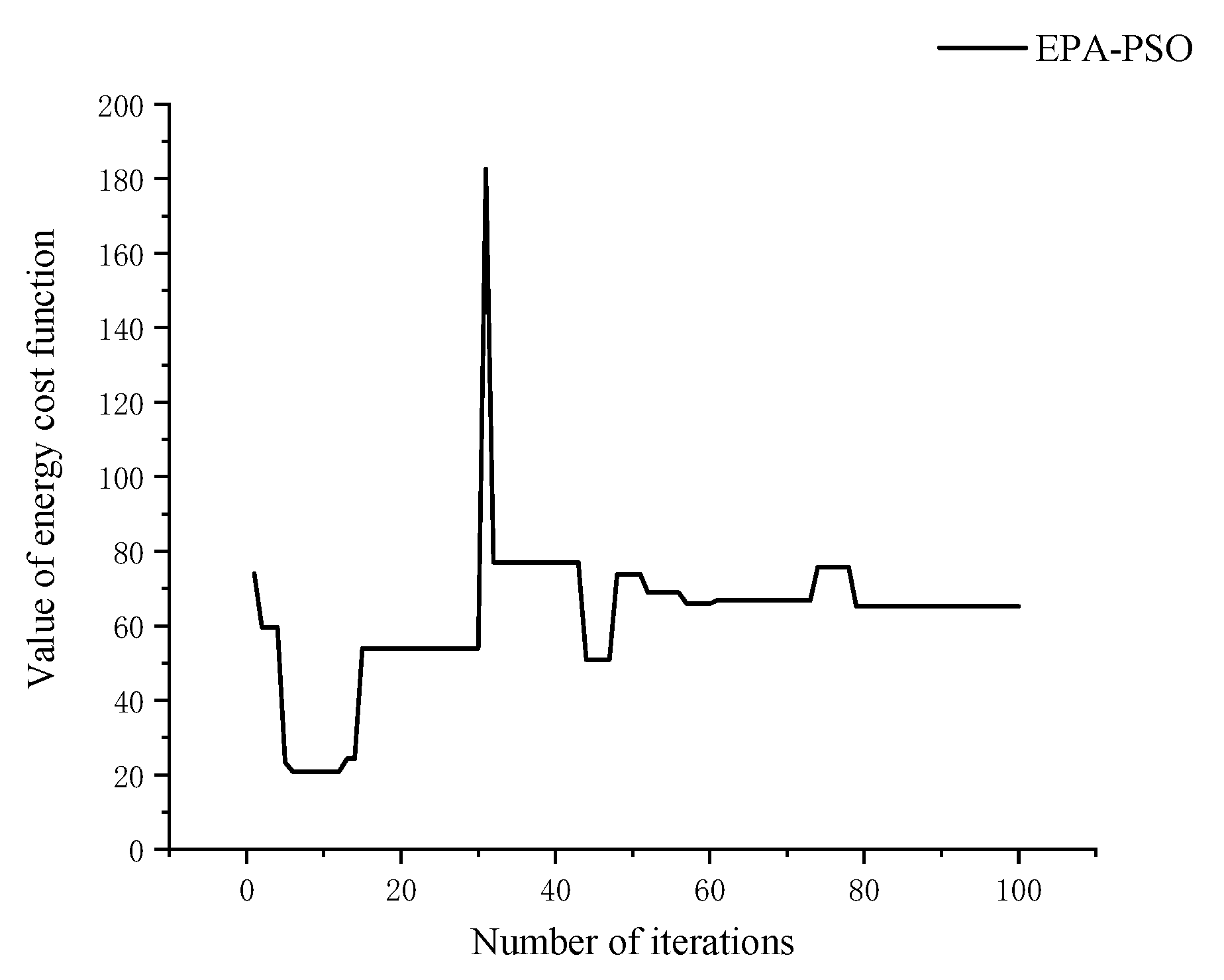
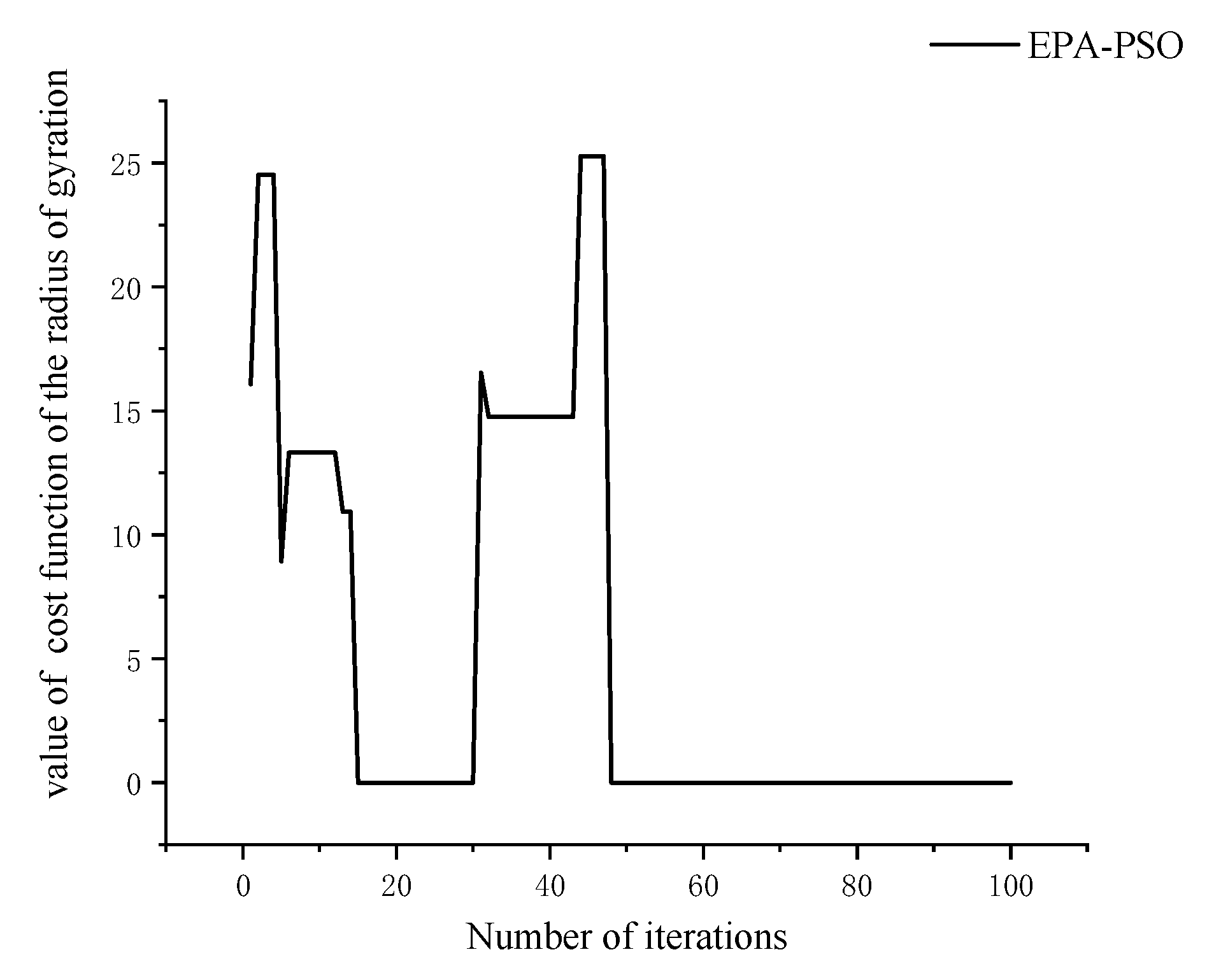
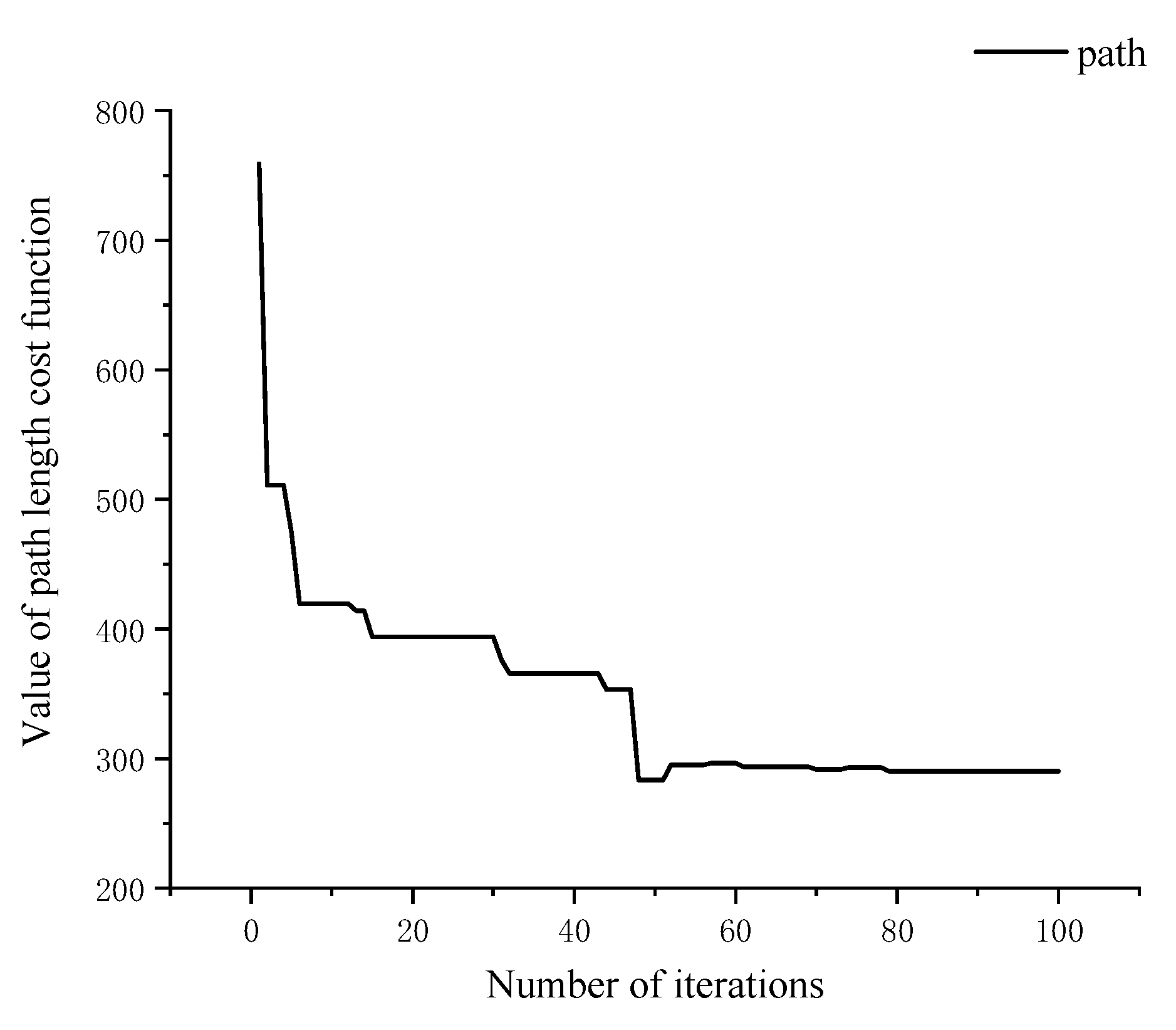
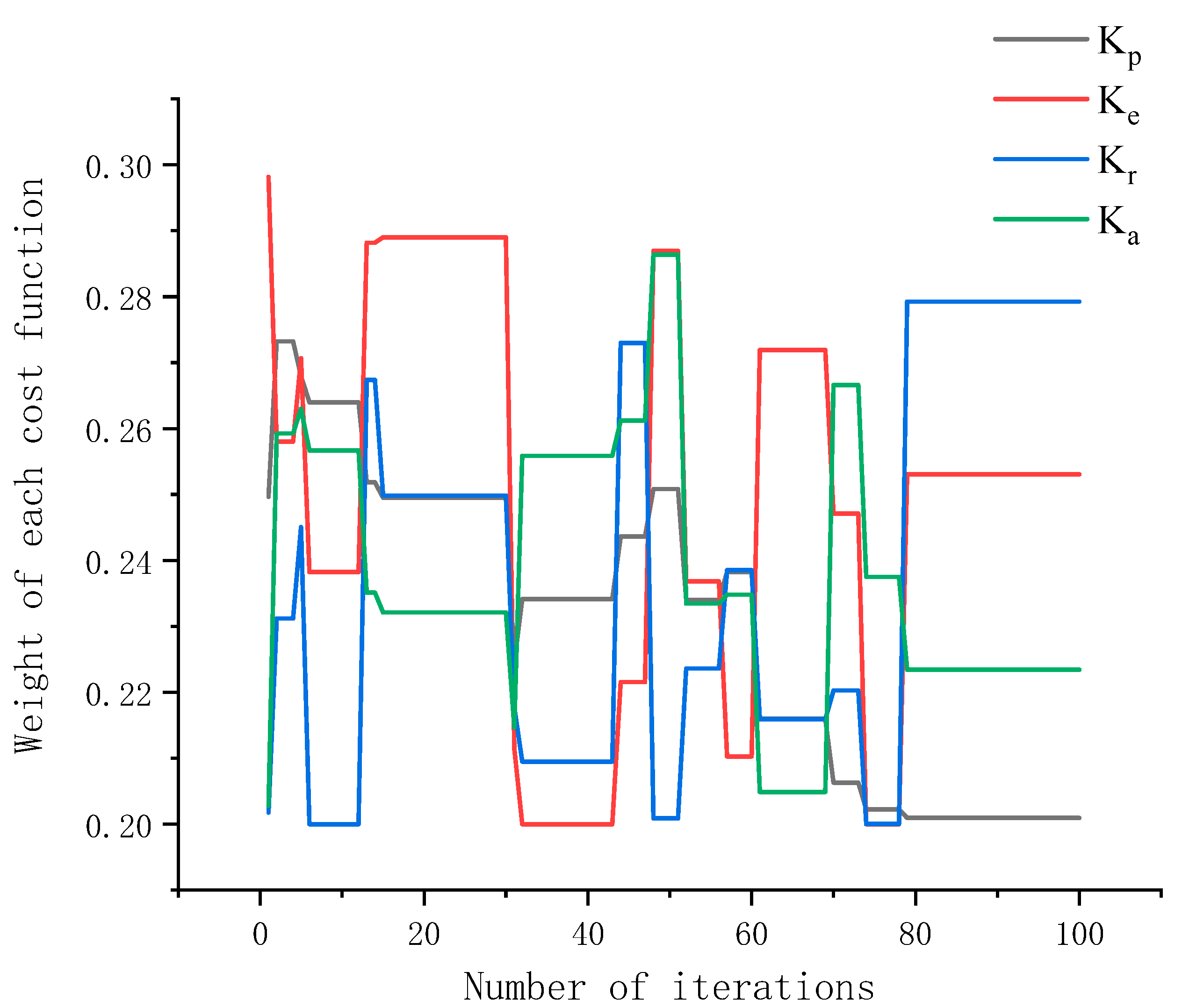
From Figure 31, Figure 32, Figure 33, Figure 34 and Figure 35, the path length planned by the EPA-PSO algorithm is 290.31 m, and the actual straight-line distance is 258.40 m. The energy consumption obtained by the EPA-PSO algorithm is 65.18. Meanwhile, the planned path points all satisfy the constraints of the minimum turning radius of AUV, namely , the planned time is 407.12 s, the actual AUV completes the planned task with a path length of 392.93 m, and the total process energy consumption is 156.64, .
According to the experimental results, it can be verified that the EPA-PSO algorithm can obtain a reliable path in the sea test experiment with a low flow rate, but if the actual marine environment is harsh, the result will become unreliable; meanwhile, for the curve shown in Figure 27, due to the error of the actual AUV motion control, the final tracking effect is not satisfactory, which also leads to the AUV consuming more energy and sailing a longer distance in the tracking task. The next step is to continue to study how to improve the control performance of AUV, so that AUV can track the optimal route planned by EPA-PSO algorithm as much as possible, and achieve the purpose of further reducing energy consumption during navigation.
6. Conclusions
We propose a multi-constraint EPA-PSO algorithm based on path length constraint, energy consumption constraint, and AUV mobility constraint. The algorithm finally determines the optimal solution in the feasible solution set, which can effectively solve the problem that the traditional PSO algorithm is prone to premature development and falls into the local optimal solution. Simulation experiments also show that the algorithm can effectively reduce the navigation energy consumption of AUV, and plan a path that satisfies the actual maneuverability of AUV. The EPA-PSO algorithm reduces the control cost, which is of great significance to reduce the operation difficulty of AUV and improve the endurance of AUV. The traditional PSO algorithm, which only considers the path length constraint, cannot satisfy the requirements of maneuverability and will consume more energy in the complex marine environment. Although M-PSO can solve the corresponding problems to a certain extent, its adjustment of constraints is random, and there is also the problem that the traditional PSO algorithm easily falls into the local optimal solution. In this paper, the superiority of the proposed EPA-PSO algorithm in planning under multi-constraint conditions is verified by simulation. Although the path length planned by EPA-PSO algorithm increases, it is of great practical value to plan a path that is more energy-saving and more in line with AUV mobility. The feasibility of the EPA-PSO algorithm is also verified in the field test in Shanghai. The next step is to further improve the control performance of AUV, make it track the path planned by EPA-PSO algorithm as much as possible, and achieve the purpose of further saving energy and reducing control cost.
Author Contributions
Data curation, G.Z.; Formal analysis, Y.S.; Investigation, X.R.; Methodology, J.L.; Resources, G.Z.; Supervision, P.C.; Writing—original draft, J.L.; Writing—review & editing, J.L. All authors have read and agreed to the published version of the manuscript.
Funding
This research was funded by the Key projects of Heilongjiang Provincial Nature Fund (Grant ZD2020E005), Shaanxi Provincial Water Conservancy Science and technology plan project (Grant 2020slkj-5). The research team greatly appreciate the support from the aforementioned institutions.
Institutional Review Board Statement
Not applicable.
Informed Consent Statement
Not applicable.
Data Availability Statement
Not applicable.
Conflicts of Interest
The authors declare no conflict of interest.
References
- Wynn, R.B.; Huvenne, V.A.I.; Bas, T.P.; Murton, B.J.; Connelly, D.P.; Bett, B.J.; Ruhl, H.A.; Morris, K.J.; Peakall, J.; Parsons, D.R. Autonomous Underwater Vehicles (AUVs): Their past, present and future contributions to the advancement of marine geoscience. Mar. Geol. 2014, 352, 451–468. [Google Scholar] [CrossRef] [Green Version]
- Aras, M.S.M.; Mazlan, K.; Ahmad, A.; Azmi, N. Analysis performances of laser range finder and blue LED for autonomous underwater vehicle (AUV). In Proceedings of the 2016 IEEE International Conference on Underwater System Technology: Theory and Applications (USYS), Penang, Malaysia, 13–14 December 2016; pp. 171–176. [Google Scholar]
- Jawhar, I.; Mohamed, N.; Al-Jaroodi, J.; Zhang, S. An architecture for using autonomous underwater vehicles in wireless sensor networks for underwater pipeline monitoring. IEEE Trans. Ind. Inform. IEEE T IND INFORM 2018, 15, 1329–1340. [Google Scholar] [CrossRef]
- Yao, T.T.; He, T.; Zhao, W.L.; Sani, A.Y.M. Review of path planning for autonomous underwater vehicles. In Proceedings of the 2019 International Conference on Robotics, Intelligent Control and Artificial Intelligence, Shanghai, China, 20–22 September 2019; pp. 482–487. [Google Scholar]
- Kirsanov, A.; Anavatti, S.G.; Ray, T. Path planning for the autonomous underwater vehicle. In Proceedings of the International Conference on Swarm, Evolutionary, and Memetic Computing, Chennai, India, 19–21 December 2013; Volume 8298, pp. 476–486. [Google Scholar]
- Liang, S.; Zhi-Ming, Q.; Heng, L.A. survey on route planning methods of AUV considering influence of ocean current. In Proceedings of the 2018 IEEE 4th International Conference on Control Science and Systems Engineering (ICCSSE), Wuhan, China, 21–23 August 2018; pp. 288–295. [Google Scholar]
- Cheng, C.; Zhu, D.; Sun, B.; Chu, Z.; Nite, J.; Sheng, Z. Path planning for autonomous underwater vehicle based on artificial potential field and velocity synthesis. In Proceedings of the 2015 IEEE 28th Canadian Conference on Electrical and Computer Engineering (CCECE), Quebec, QC, Canada, 13–16 May 2018; pp. 717–721. [Google Scholar]
- Taheri, E.; Ferdowsi, M.H.; Danesh, M. Closed-loop randomized kinodynamic path planning for an autonomous underwater vehicle. Appl. Ocean Res. 2019, 83, 48–64. [Google Scholar] [CrossRef]
- Guo, Y.; Liu, H.; Fan, X.; Lyu, W. Research Progress of Path Planning Methods for Autonomous Underwater Vehicle. Math. Probl. Eng. 2021, 2021. [Google Scholar] [CrossRef]
- Wei, D.; Wang, F.; Ma, H. Autonomous path planning of AUV in large-scale complex marine environment based on swarm hyper-heuristic algorithm. Appl. Sci. 2019, 9, 2654. [Google Scholar] [CrossRef] [Green Version]
- Koay, T.B.; Chitre, M. Energy-efficient path planning for fully propelled AUVs in congested coastal waters. In Proceedings of the 2013 MTS/IEEE OCEANS-Bergen, Bergen, Norway, 10–14 June 2013; pp. 1–9. [Google Scholar]
- Yao, P.; Zhao, S. Three-dimensional path planning for AUV based on interfered fluid dynamical system under ocean current (June 2018). IEEE Access 2018, 6, 42904–42916. [Google Scholar] [CrossRef]
- Saad, M.; Salameh, A.I.; Abdallah, S. Energy-efficient shortest path planning on uneven terrains: A composite routing metric approach. In Proceedings of the 2019 IEEE International Symposium on Signal Processing and Information Technology (ISSPIT), Ajman, United Arab Emirates, 10–12 December 2019; pp. 1–6. [Google Scholar]
- Sun, B.; Zhang, W.; Li, S.; Zhu, X.X. Energy optimised D* AUV path planning with obstacle avoidance and ocean current environment. J. Navig. 2022, 1–20. [Google Scholar] [CrossRef]
- Jones, D.; Hollinger, G.A. Planning energy-efficient trajectories in strong disturbances. IEEE Robot. Autom. Lett. 2017, 2, 2080–2087. [Google Scholar] [CrossRef]
- Li, J.; Yang, C. AUV path planning based on improved RRT and bezier curve optimization. In Proceedings of the 2020 IEEE International Conference on Mechatronics and Automation (ICMA), Beijing, China, 2–5 August 2020; pp. 1359–1364. [Google Scholar]
- Zeng, Z.; Sammut, K.; Lian, L.; He, F.; Lammas, A.; Tang, Y. A comparison of optimization techniques for AUV path planning in environments with ocean currents. Robot. Auton. Syst. 2016, 82, 61–72. [Google Scholar] [CrossRef]
- Tanakitkorn, K.; Wilson, P.A.; Turnock, S.R.; Phillips, A.B. Grid-based GA path planning with improved cost function for an over-actuated hover-capable AUV. In Proceedings of the 2014 IEEE/OES Autonomous Underwater Vehicles (AUV), Oxford, MS, USA, 6–9 October 2014; pp. 1–8. [Google Scholar]
- Ma, Y.N.; Gong, Y.J.; Xiao, C.F.; Gao, Y.; Zhang, J. Path planning for autonomous underwater vehicles: An ant colony algorithm incorporating alarm pheromone. IEEE Trans. Veh. Technol. 2018, 68, 141–154. [Google Scholar] [CrossRef]
- Wang, Z.; Xiang, X.; Yang, J.; Yang, S. Composite Astar and B-spline algorithm for path planning of autonomous underwater vehicle. In Proceedings of the 2017 IEEE 7th International Conference on Underwater System Technology: Theory and Applications (USYS), Kuala Lumpur, Malaysia, 18–20 December 2017; pp. 1–6. [Google Scholar]
- Zhang, L.; Zhang, L.; Liu, S.; Zhou, J.; Papavassiliou, C. Three-dimensional underwater path planning based on modified wolf pack algorithm. IEEE Access 2017, 5, 22783–22795. [Google Scholar] [CrossRef]
- Chen, G.; Shen, Y.; Qu, N.; He, B. Path planning of AUV during diving process based on behavioral decision-making. Ocean Eng. 2021, 234, 109073. [Google Scholar] [CrossRef]
- Mahmoudzadeh, S.; Yazdani, A.M.; Sammut, K. Powers D M W. Online path planning for AUV rendezvous in dynamic cluttered undersea environment using evolutionary algorithms. Appl. Soft Comput. 2018, 70, 929–945. [Google Scholar] [CrossRef] [Green Version]
- Che, G.; Liu, L.; Yu, Z. An improved ant colony optimization algorithm based on particle swarm optimization algorithm for path planning of autonomous underwater vehicle. J. Ambient Intell. Humaniz. Comput. 2020, 11, 3349–3354. [Google Scholar] [CrossRef]
Figure 1.
AUV motion coordinate system.

Figure 2.
Steps of EPA-PSO algorithm.

Figure 3.
Simulated environment obstacles.

Figure 4.
Fitness of PSO algorithm.

Figure 5.
Fitness of M-PSO algorithm.

Figure 6.
Fitness of EPA-PSO algorithm.

Figure 7.
Inertia weight.

Figure 8.
Learning efficiency.

Figure 9.
The trust of particles in speed jump.

Figure 10.
The weight of cost function of EPA-PSO algorithm after 100 iterations.

Figure 11.
The weight of cost function of EPA-PSO algorithm after 200 iterations.

Figure 12.
The weight of cost function of EPA-PSO algorithm after 500 iterations.

Figure 13.
Numerical comparison of energy cost functions after 100 iterations.

Figure 14.
Numerical comparison of energy cost functions after 200 iterations.

Figure 15.
Numerical comparison of energy cost functions after 500 iterations.

Figure 16.
Numerical comparison of cost functions of radius of gyration after 100 iterations.

Figure 17.
Numerical comparison of cost functions of radius of gyration after 200 iterations.

Figure 18.
Numerical comparison of cost functions of radius of gyration after 500 iterations.

Figure 19.
Numerical comparison of cost functions of trim angle after 100 iterations.

Figure 20.
Numerical comparison of cost functions of trim angle after 200 iterations.

Figure 21.
Numerical comparison of cost functions of trim angle after 500 iterations.

Figure 22.
3D path planning after 100 iterations.

Figure 23.
3D path planning after 200 iterations.

Figure 24.
3D path planning after 500 iterations.

Figure 25.
Radar chart of value of cost function.

Figure 26.
An AUV of Harbin Engineering University.

Figure 27.
AUV path planned for the field test.

Figure 28.
AUV standby in dock.

Figure 29.
AUV during autonomous operation.

Figure 30.
AUV performs depth determination task.

Figure 31.
Fitness of EPA-PSO algorithm after 100 iterations.

Figure 32.
Value of energy cost function of EPA-PSO algorithm after 100 iterations.

Figure 33.
The value of cost function of the radius of gyration of the EPA-PSO algorithm after 100 iterations.
Figure 33.
The value of cost function of the radius of gyration of the EPA-PSO algorithm after 100 iterations.

Figure 34.
The value of path cost function of EPA-PSO algorithm after 100 iterations.

Figure 35.
The weight of cost function of EPA-PSO algorithm after 100 iterations.


Table 1.
Description of system parameters.
| Physical Quantity | -axis | -axis | -axis |
|---|---|---|---|
| Velocity | |||
| Angular velocity | |||
| Force | |||
| Torque |
Table 2.
Values of the initial parameters.
| 8 m | −20° | 20° | 500 |
| 0.25 | 0.01 | 0.25 | 0.01 |
| 0.25 | 0.01 | 0.25 | 0.01 |
| 1.2 | 1.5 | 1.5 | 2.5 |
| 10 | 10 | 10 | 10 |
| 50 | 100/200/500 | −20 | 20 |
| / | |||
| 0.8 | 2.5 | 1.5 | 15 |
Table 3.
The numerical analysis of cost function.
| Method | Fitness | |||||
|---|---|---|---|---|---|---|
| 100 iterations | PSO | 93.81 | 280.36 | 77.81 | 283.50 | 93.81 |
| M-PSO | 92.87 | 104.68 | 32.05 | 48.87 | 185.87 | |
| EPA-PSO | 80.76 | 81.83 | 24.29 | 41.73 | 206.58 | |
| 200 iterations | PSO | 96.23 | 335.12 | 71.39 | 194.20 | 96.23 |
| M-PSO | 92.07 | 123.28 | 15.67 | 43.52 | 187.80 | |
| EPA-PSO | 67.44 | 83.19 | 12.39 | 42.77 | 195.14 | |
| 500 iterations | PSO | 93.41 | 334.00 | 43.02 | 268.97 | 93.41 |
| M-PSO | 96.61 | 87.00 | 27.24 | 52.05 | 220.12 | |
| EPA-PSO | 65.71 | 60.16 | 8.75 | 25.01 | 218.81 |
Table 4.
The table of fitness correction.
| Method | ||
|---|---|---|
| 100 iterations | PSO | 183.87 |
| M-PSO | 92.87 | |
| EPA-PSO | 88.60 | |
| 200 iterations | PSO | 174.24 |
| M-PSO | 92.07 | |
| EPA-PSO | 83.37 | |
| 500 iterations | PSO | 248.42 |
| M-PSO | 109.71 | |
| EPA-PSO | 79.43 |
Publisher’s Note: MDPI stays neutral with regard to jurisdictional claims in published maps and institutional affiliations. |
© 2022 by the authors. Licensee MDPI, Basel, Switzerland. This article is an open access article distributed under the terms and conditions of the Creative Commons Attribution (CC BY) license (https://creativecommons.org/licenses/by/4.0/).
Share and Cite
MDPI and ACS Style
Zhang, G.; Liu, J.; Sun, Y.; Ran, X.; Chai, P. Research on AUV Energy Saving 3D Path Planning with Mobility Constraints. J. Mar. Sci. Eng. 2022, 10, 821. https://0-doi-org.brum.beds.ac.uk/10.3390/jmse10060821
AMA Style
Zhang G, Liu J, Sun Y, Ran X, Chai P. Research on AUV Energy Saving 3D Path Planning with Mobility Constraints. Journal of Marine Science and Engineering. 2022; 10(6):821. https://0-doi-org.brum.beds.ac.uk/10.3390/jmse10060821
Chicago/Turabian StyleZhang, Guocheng, Jixiao Liu, Yushan Sun, Xiangrui Ran, and Puxin Chai. 2022. "Research on AUV Energy Saving 3D Path Planning with Mobility Constraints" Journal of Marine Science and Engineering 10, no. 6: 821. https://0-doi-org.brum.beds.ac.uk/10.3390/jmse10060821
Note that from the first issue of 2016, this journal uses article numbers instead of page numbers. See further details here.