Optimization of a Regional Marine Environment Mobile Observation Network Based on Deep Reinforcement Learning

Abstract

The observation path planning of an ocean mobile observation network is an important part of the ocean mobile observation system. With the aim of developing a traditional algorithm to solve the observation path of the mobile observation network, a complex objective function needs to be constructed, and an improved deep reinforcement learning algorithm is proposed. The improved deep reinforcement learning algorithm does not need to establish the objective function. The agent samples the marine environment information by exploring and receiving feedback from the environment. Focusing on the real-time dynamic variability of the marine environment, our experiment shows that adding bidirectional recurrency to the Deep Q-network allows the Q-network to better estimate the underlying system state. Compared with the results of existing algorithms, the improved deep reinforcement learning algorithm can effectively improve the sampling efficiency of the observation platform. To improve the prediction accuracy of the marine environment numerical prediction system, we conduct sampling path experiments on a single platform, double platform, and five platforms. The experimental results show that increasing the number of observation platforms can effectively improve the prediction accuracy of the numerical prediction system, but when the number of observation platforms exceeds 2, increasing the number of observation platforms will not improve the prediction accuracy, and there is a certain degree of decline. In addition, in the multi-platform experiment, the improved deep reinforcement learning algorithm is compared with the unimproved algorithm, and the results show that the proposed algorithm is better than the existing algorithm.

1. Introduction

The adaptive sampling technology of marine environment observation platforms is an important part of the marine environment monitoring system. Marine environment observation data play an important role in improving the prediction accuracy of the marine environment numerical prediction system. Due to the limited coverage and high cost of direct observation, it is unrealistic to carry out large-scale and long-term observation. The limited observation resources have become the main obstacle restricting the development of regional complex marine environment observation and prediction technology. A subject of scientific importance is the use of a mobile observation platform to realize the adaptive sampling of sensitive data from the complex marine environment and improve the prediction accuracy of marine environment monitoring and forecasting systems.

In the past few decades, path planning technology for marine environment observation has made great progress. Due to the complexity and time variability of the marine environment and the diversity of unmanned survey vessels (USVs) used in underwater road strength planning tasks, the adaptive sampling of the marine environment observation platform needs more safe and efficient path planning technology to ensure the smooth completion of the task.

The ocean observation system plays an important role in understanding and managing the ocean. Marine environment mobile platform observation technology is an important part of marine observation systems [1]. Marine environmental information has the characteristics of multiple sources, timeliness, massive data, and unequal spatial and temporal scales. The effective collection of marine environmental information is an important issue in marine environmental observation [2].

The validity of the sampling data from marine environment mobile platform observation systems has a great influence on the accuracy of marine environment field prediction. Due to the limited ocean observation resources, in the actual sampling process, to improve the sampling efficiency, factors such as the complex and diverse sources of marine environmental information, random dynamics, and high-dimensional states need to be considered, especially for the collection of regional information containing large dynamic changes and uncertainties [3,4,5,6,7,8].

The traditional marine environment mobile observation network optimization plan, based on the acquired marine element analysis and forecast field data, uses the measurement attributes of the marine mobile observation platform, the collision avoidance and overlap constraints between the mobile observation platform groups, etc., to construct the deployment plan of the mobile observation network global cost function. A suitable global optimization algorithm, such as the genetic algorithm, particle swarm algorithm, ant colony algorithm, etc., is selected to solve the optimized observation path of the mobile observation network, and to verify its effect on the improvement of marine environment analysis and forecasting capabilities. The real-time observation information obtained by the observation network updates the analysis and forecast information of marine environmental elements, and the updated background field can re-plan a new mobile observation network deployment plan [8,9,10,11,12]. The advantages of this scheme are that it is clear and the technical route is easy to implement, but the disadvantages are that it needs to construct a complex cost function, human subjective factors are large, it is difficult to find a reasonable global optimization algorithm, and the planning results often cannot meet actual needs.

Therefore, how to build a marine environment mobile observation network based on a limited marine environment observation platform to achieve the optimal observation of the regional marine environment, and how to realize the adaptive path of the marine environment observation platform based on the real-time marine environment observation data obtained by the marine mobile observation platform optimization have become important issues in the current development of regional marine environment observation technology.

This paper uses the deep reinforcement learning algorithm for the design of a regional marine environment observation network for the first time. Deep reinforcement learning is a sequential decision algorithm. Aiming to address the drawbacks of traditional optimization methods, the adaptive observation of the marine environment is regarded as a type of sequential decision-making optimization problem. The regional marine environment mobile observation platform receives instructions and takes the next step by acquiring the current complex marine environment background information to realize the optimal observation of the complex marine environment. Reinforcement learning algorithm is a method of learning, prediction, and decision making. The optimal strategy is learned through trial and error through the interaction between the agent and the environment. The reinforcement learning algorithms have been widely used in path planning.

Reinforcement learning (RL), another research hotspot in the field of machine learning, has been widely used in industrial manufacturing [13], simulation [14], robot control [15], optimization and scheduling [16], and gaming [17], in addition to other fields. The basic idea of RL is to learn the optimal strategy for accomplishing the goal by maximizing the accumulated reward value obtained by the agent from the environment.

Chao et al. [18], using deep reinforcement learning for UAV path planning in dynamic environments, applied the D3QN algorithm to predict the Q value of candidate actions, and used greedy strategies and heuristic search rules for action selection, making it suitable for static performance under dynamic tasks. Wen et al. [19] used active SLAM technology, the dueling deep reinforcement learning algorithm for path planning, and the FastSLAM algorithm to locate and map the environment to realize the autonomous navigation of robots in complex environments. Yao et al. [20] used reinforcement learning to improve the artificial potential field method and solved the local stable point scene by combining the improved black hole potential field and reinforcement learning. Li et al. [21] used deep reinforcement learning to plan the UAV’s ground target tracking path. In this method, the DDPG algorithm is improved, and a reward function based on the line of sight and artificial potential field is constructed, so that the UAV can effectively maintain target tracking, avoid obstacles, and reduce the failure rate. Jiang et al. [22] used deep reinforcement learning to plan the path of asteroid jumping, and improved the DQN architecture to determine the best action for jumping, combining three structural elements to improve the performance of the DRL algorithm, making learning more efficient, and solving the path planning problem. Wang et al. [23] adopted the hierarchical path planning method of Global Guided Reinforcement Learning (G2RL) to plan the path of mobile robots in large dynamic environments, with good versatility and scalability. Wei et al. [24] applied reinforcement learning to information path planning (IPP), and developed a constrained exploration and development strategy to deal with the information collection path planning problem of mobile robots with sensing and navigation functions and to improve their work efficiency. Shirel Josef et al. [25] applied DRL to the navigation of unmanned ground vehicles, used zero-distance to local range perception to perform local navigation on unknown rugged terrain, and used reward plasticity to provide dense reward signals. The simulated method is able to navigate on surfaces with different levels of friction.

This article makes the following three contributions:

• Using reinforcement learning, we build a marine environment. Traditional algorithms need to construct a complex ocean environment cost function, while reinforcement learning uses the characteristics of ocean environment elements to build the ocean environment. In the marine environment created by the deep learning network, the agent can learn by interacting with the environment to achieve its goals;
• To cope with the partial observability of the observation environment, we use the Dueling Double Deep Recurrent Q-network (D3RQN) algorithm to approximate the optimal value function. Algorithms based on D3RQN can solve partially observable problems through bidirectional recurrent neural networks. This method is more robust than the Deep Q-network (DQN), Dueling Double Deep Q-network (D3QN), and Deep Recurrent Q-network (DRQN) methods in the ways that the neural network with a bidirectional layer can learn the pre-order environment state and the reverse order environment state at the same time, and thus the sampling results obtained by the platforms are closer to the true value;
• Planning the observation path of the mobile observation network through deep reinforcement learning can improve the observation efficiency of marine environment elements and the ability to analyze and forecast under the condition of limited observation resources. When the number of observation platforms exceeds 2, the assimilation results will not be significantly improved.

The chapters of this article are arranged as follows: in Section 2, basic knowledge, including the refined analysis and forecasting of the regional coupling environment, that is, the acquisition model of the marine environment background field, the motion model of the mobile observation platform, and the introduction of deep reinforcement learning algorithms, is provided; in Section 3, we propose the self-adaptive optimization algorithm of the regional marine environment mobile observation network based on deep reinforcement learning, including data processing methods, environment construction, reward function design, and neural network construction; in Section 4, we provide the simulation experiment results and analysis, which proves the feasibility and effectiveness of the algorithm used in regional marine environment observation; and in Section 5, we give the summary and outlook.

2. Method

2.1. Refined Analysis and Forecast of Regional Coupling Environment

Before proceeding with the design and research of the observation plan of the regional ocean mobile observation network, it is first necessary to construct a regional coupling/marine environment numerical forecast system to realize the analysis and forecast of the coupling/marine environment elements. This article chooses to make corresponding changes and adjustments based on a medium-complexity coupled circulation mode (ICCM) [26]. This ICCM has energy conservation characteristics, so it has unique advantages in simulating the process of the evolution of atmospheric, ocean, and land temperature. Here, we select parts of the Northwest Pacific Ocean as the sea area to be measured and take temperature changes as the research object to explore the intelligent optimization design of the optimal observation plan of the regional ocean mobile observation network. Based on the multi-level nested regional coupling model system, and using a coupled data assimilation method that combines the optimal observation time window and a coupled multi-parameter synchronization optimization method, determined by the sensitivity of model parameters, a regional coupled environment analysis and forecasting system is constructed. We realize the analysis and forecasting of the regional coupling/marine environment, and output the analysis and forecast information of sea surface temperature for the next 5 days.

2.2. Regional Marine Environment Mobile Observation Network Model

The regional marine environment mobile observation network is composed of unmanned survey vessels (USVs), buoys, etc. [27]. The objects of observation are areas in the ocean with large temperature differences under a certain time gradient. This article mainly discusses the observation path planning for the sampling points of the unmanned survey ship in the ocean. As shown in Figure 1, the USV should start from the selected starting point $(x_1,y_1)$, measure the area where the temperature difference in the ocean changes greatly, and control the USV in real time based on unknown obstacles to avoid collisions. The aim is to maximize the sampling of points with large temperature changes within the range of the region under constrained conditions. The path from one point $(x_i,y_i)$ to another point $(x_{i+1},y_{i+1})$ can be expressed by the following formula:

$$\left\{\begin{array}{cc}\hfill x_{i+1}& =x_i+v_{i}t·cos\left(\theta \right)\hfill \\ \hfill y_{i+1}& =y_i+v_{i}t·sin\left(\theta \right)\hfill \end{array}\right.$$

(1)

where $\theta$ is the heading angle of the USV at the ith waypoint; $v_i$ is the speed of the USV at the ith waypoint; and t is the time step.

The schematic diagram of the USV’s marine environment detection is shown in Figure 1. The USV detects the surrounding marine environment in a certain direction. The detection angle is $\alpha$, the detection radius is R, and the detected temperature difference in the sampling point is $(\Delta T_{i1},\Delta T_{i2},\Delta T_{im})$. The temperature difference is compared, and the sampling point of the next point $\Delta T_{ij}$ is selected as the largest temperature difference. d represents the gradient function, and z and f represent the objective function. Therefore, for this problem, the objective function is

$$\begin{array}{cc}\hfill \mathbf{max}& z=\sum \Delta T_i\hfill \\ \hfill \mathbf{s}.\mathbf{t}& d=d\left(T_i\right)\hfill \\ \hfill & 0\le v_i\le v_{max}\hfill \\ \hfill & {\theta }_1\le {\theta }_i\le {\theta }_2\hfill \\ \hfill & i=1,2,...,n\hfill \end{array}$$

(2)

2.3. Partially Observable Markov Decision Process

The Partially Observable Markov Decision Process (POMDP) is a generalized Markov decision process [28]. The decision-making procedure of the POMDP simulation agent assumes that the system dynamics are determined by the MDP, but the agent cannot directly observe the state. On the contrary, it must infer the distribution of states based on the observations of the whole and partial regions of the model. Formally, POMDP is a 7-tuple process $\left(S,A,T,R,\mathsf{\Omega },O,\gamma \right)$, in which S, A, T, R, and $\mathsf{\Omega }$ are the states, actions, conditional transition probability, reward functions, and observations, respectively. O is the conditional observation probability. $\gamma$ is the discount factor. The agent is not receiving observations at each step s${}_t$, but is receiving observations at o${}_t$. The discount factor $\gamma$ determines how much of a direct reward is gained for greater distances. When $\gamma$ = 0, the agent only cares about which action would produce the largest expected instant reward; when $\gamma$ = 1, the agent is concerned with maximizing the expected sum of future rewards.

In our problem, the background field of the observation platform during the sampling process changes with time. For a certain period, the observation platform is not sure which state it is in. The observation platform first needs to determine what state it is in before it can decide to sample. Therefore, our problem is a POMDP [29].

We assume that the state of the observation platform at each moment obeys the $O\left(o\right|s)$ distribution. After the observation platform observes the data o, the probability of determining the state s is $O\left(o\right|s)$. The observation platform will proceed to the next action a according to the state it is in. $P\left(s^{\prime }\right)|s,a$ indicates the probability of reaching state $s^{\prime }$ after the observation platform performs action a. $R(s,a)$ represents the reward for performing the action. Our goal is to choose the action a of each step for the observation platform to maximize the cumulative return value: $E\left[{\sum }_{t=0}^{\infty }{\gamma }^t{r}_t\right]$. We take $\gamma =0.99$, because we are more concerned with the sum of the benefits of the future work of the observation platform.

2.4. Deep Q-Network

Reinforcement learning [30] is one of the paradigms and methodologies of machine learning. It is used to describe and solve the problem of how the agent interacts with the environment through learning. Such strategies aim to maximize returns or achieve specific goals.

The common model of reinforcement learning is the standard Markov Decision Process (MDP). According to given conditions, reinforcement learning can be divided into model-based RL and model-free RL, as well as active RL and passive RL. The variants of reinforcement learning include reverse reinforcement learning, hierarchical reinforcement learning, and observable system reinforcement learning. The algorithms used to solve reinforcement learning problems can be divided into two categories: strategy search algorithms and value function algorithms. Deep learning models can be used in reinforcement learning to form deep reinforcement learning.

Deep reinforcement learning (DRL) [31] combines the perception ability of deep learning with the decision-making ability of reinforcement learning, which can be directly controlled according to the input image. It is an artificial intelligence method that can be considered closer to human thinking.

The main algorithm flow of DQN is to combine the neural network with the Q-network algorithm, use the neural network’s powerful image representation ability, and use video frame data as the state in reinforcement learning and as the input of the neural network model; then, the neural network model outputs every value (Q value) corresponding to each action, causing the action to be executed. As shown in Figure 2, we take the forecast data obtained through ICCM and the observation platform as the environment, and the proposed D3RQN as the algorithm model of the agent. Our task is to allow the agent to obtain greater rewards in the interaction with the environment, that is, the observation platform adopts more valuable samples.

The DQN algorithm uses a deep convolutional network with a weight parameter of $\theta$ as the network model of the action value function. The action value function $Q(s,a,\theta )$ is simulated by the convolutional neural network model $Q^{\pi }(s,a)$, as follows:

$$Q(s,a,\theta )=Q^{\pi }(s,a)$$

(3)

We use the mean square error to define the objective function as the loss function of the deep convolutional neural network, the formula for which is as follows:

$$\begin{array}{c}L(s,a|{\theta }_i)={(r+\gamma m_{\alpha }xQ(s^{\prime },a^{\prime }|{\theta }_i)-Q(s,a|{\theta }_i))}^2\end{array}$$

(4)

$$\begin{array}{c}{\theta }_{i+1}={\theta }_i+\alpha {\Delta }_{\theta }L\left({\theta }_i\right)\end{array}$$

(5)

where $s^{\prime }$ and $a^{\prime }$ are the state and action of the next period, respectively.

The DQN algorithm introduces three technologies to combine deep learning and reinforcement learning: First, the objective function, which can be learned by deep learning, is constructed based on the Q-network algorithm. Second, the target Q value is generated based on the convolutional neural network, and the Q value of the next state is evaluated based on the target Q value. Third, the empirical playback mechanism is introduced to solve the problems of correlation and non-static distribution between the data. The DQN algorithm uses the mean square error to define the objective function as the loss function of the deep convolution neural network. The formula is as follows:

$$L_i\left({\theta }_i\right)=[E_{(s_t,a_t,r_t,s_{t+1})}D\left[{(y_i-Q(s_i,a_i|{\theta }_i))}^2\right]$$

(6)

where $y_i^{DQN}=r_t+\gamma ma{x}_{a^{\prime }}Q(s_{t+1},a^{\prime };{\theta }_s^{-})$ is the stale update target given by the target network $\widehat{Q}$. Updates performed in this manner have been empirically shown to be tractable and stable [32].

Hado van Hassell et al. [31] put forward the Double DQN algorithm (DDQN) by combining the idea of DQN with itself. The literature gives a general explanation of overestimation and the mathematical proof of the solution. Finally, the algorithm achieved a super high score in an experiment on an Atari game. In the DDQN algorithm, the objective function is as follows:

$$y_i^{DDQN}=r_t+\gamma Q\left(s^{\prime },\underset{a^{\prime }}{arg\max }Q\left(s^{\prime },a^{\prime };{\theta }_i\right);{\theta }^{-}\right)$$

(7)

In [33], Ziyu Wang et al. proposed a new neural network structure—the Dueling Network. The input of the network is the same as the input of the DQN and DDQN algorithms. However, the output of the Dueling DQN algorithm includes two branches, namely, the state V-value (scalar) of the state and the dominant A-value (a vector with the same dimension as the action space) of each action. In the Dueling Network, the Q-value is designated as

$$\begin{array}{cc}\hfill & Q(s,a;\theta ,\alpha ,\beta )=V(s;\theta ,\beta )+\hfill \\ \hfill & \left(A(s,a;\theta ,\alpha )-\frac{1}{\left|\mathcal{A}\right|}\sum _{a^{\prime }}A\left(s,a^{\prime };\theta ,\alpha \right)\right)\hfill \end{array}$$

(8)

where $\theta$ denotes the parameters of the volume layer, and $\alpha$ and $\beta$ are the flow parameters in the Dueling Network. $V(s;\theta ,\beta )$ is the state-action value. $A(s,a;\theta ,\alpha )$ is the action advantage value. $\frac{1}{\left|\mathcal{A}\right|}{\sum }_{a^{\prime }}A\left(s,a^{\prime };\theta ,\alpha \right)$ is the average value of the sum of the output values of the advantage function.

Dueling Double Deep Bidirectional Recurrency Q-Network

The experimental results of Matthew et al. [34] show that adding recurrency to Deep Q-learning allows the Q-network to better estimate the underlying system state, narrowing the gap between $Q(o,a|\theta )$ and $Q(s,a|\theta )$.

Wang et al. [35], by combining the advantages of the Dueling Network and DDQN algorithm, proposed the Dueling Double Deep Q-network (D3QN) to learn the decision-making strategy of typical UAVs. In that article, they used D3QN to realize the path planning of data acquisition in multi-UAV scenarios.

Our experiments show that adding bidirectional recurrency to Deep Q-learning allows the Q-network to better estimate the underlying system state, narrowing the gap between $Q(o,a|\theta )$ and $Q(s,a|\theta )$. In other words, bidirectional recurrent deep Q-networks can better approximate actual Q-values from the previous state sequence and the subsequent state sequence of observations, leading to better policies in partially observed environments. According to Formulas (6)–(8), the loss function used in this paper is as follows.

Since the problem of the adaptive observation of the marine environment is a POMDP problem, this paper adds the bidirectional recurrent neural network to D3QN algorithm to train state values. The bidirectional recurrent neural network can enable the intelligent observation platform to more fully learn the complex information in the marine environment. Combining the idea of the Dueling Network algorithm, the S value trained by this network and the dominant value are added as the next action value of the agent, as shown in Figure 3.

$$\begin{array}{c}L(\theta ,\alpha ,\beta )=\\ E\left[r_t+\gamma Q\left(s^{\prime },\underset{a^{\prime }}{argmax}Q\left(s^{\prime },a^{\prime };{\theta }_i\right);{\theta }^{-}\right)-Q(s,a;\theta ,\alpha ,\beta )\right]\end{array}$$

(9)

3. Design of a Mobile Observation Network for the Marine Environment Based on Deep Bidirectional Recurrent Reinforcement Learning

3.1. Data Collection and Processing

We train the model to find areas where the temperature difference changes significantly over time. The data predicted by the numerical model cannot be directly used for training. To obtain better training results, we need to process the original data. The data obtained by numerical prediction are irregular point data, while the convolutional neural network can only process grid structure topology data. We usually use normalization methods for data preprocessing. The purpose is to normalize the features of each dimension to the same value interval and eliminate the correlation between different features to obtain the desired result. RankGauss [36] is a variable processing method, similar to normalization (MinMax) and standardization (Standardization), both allowing the model to better fit the data. The effect of using RankGauss will also be better than normalization and standardization. Through numerical forecasting, we predict 11 sets of data for 5 days.

The observation platform makes observations every six hours, and can observe a total of 21 points in 5 days. First, we need to interpolate 11 sets of original data to obtain 21 sets of new data. Then, we use RankGauss to preprocess 21 sets of data to obtain the global background field. Third, we process 21 sets of data according to the time gradient to obtain 20 sets of data, and preprocess the time gradient field by the RankGauss method. Figure 4 shows the data processing method, the original data, the time gradient data, and the data processed by RankGauss. Due to space limitations, this paper show four pieces of data for each type of processing.

3.2. State Space and Action Space

To achieve the purpose of sampling in the regional marine environment, the observation platform needs to obtain at least three pieces of information, i.e., the status information of the observation platform itself, the relationship between the observation platform and the environment, and the number of observation platforms sampled. First, the observation platform needs to confirm the position of the background field where it is. Since the background field is dynamic, as explained in Section 2.3, the observation platform also needs to confirm its own background field. We use a set of parameters $O=[o_1,o_2,\cdots ,o_{21}]$ to confirm the background field where the observation platform is located. After confirming the background field, we then confirm the position $(x,y)$ of the observation platform in the current background field. It is then necessary to confirm the relationship between the observation platform and the surrounding environment. By confirming the speed and direction of the observation platform, we can determine the location of the observation platform and perform sampling. We use a vector $[\alpha ,v]$ to represent the distance and direction between the current position of the observation platform and the next sampling point. Deep reinforcement learning to solve sequential decision-making problems generally requires the action space of the agent to be discrete. The direction angle of the observation platform is set as a discrete action, and we set $\xi =[-{45}^{\circ },-{30}^{\circ },$$-{15}^{\circ },0^{\circ },{15}^{\circ },{30}^{\circ },{45}^{\circ }]$. The speed is constant, $v=5$. Lastly, we use the vectors $T=[T_1,T_2,\cdots ,T_8]$ to represent the relationship between the observation platform and the sampling points. According to the data processing in Section 3.1, we divide the sampling points into eight parts according to their size, so we use vectors $T=[T_1,T_2,\cdots ,T_8]$ to represent the sampling quality of the observation platform.

3.3. Reward Function

The reward function is a signal used to evaluate whether the action taken by the agent in the environment is good or bad. For the observation platform sampling in the complex and dynamic marine environment, because we need to evaluate the sampling quality, we design a sparse reward. When the observation platform reaches a sampling point, it returns a reward until all sampling is completed, with the goal to maximize all samples.

The design of the reward function in this article involves many factors. The reward function mainly consists of three parts in the marine environmental information gradient: observation platform measurement attribute constraints, observation platform obstacle avoidance constraints, and the collision constraint between observation platforms.

First, we consider the reward function of the time gradient for marine environmental elements. The background field data are preprocessed according to the temperature gradient change characteristics of the area to be observed. Section 3.1 introduces the data preprocessing method. According to the data processing results, the goal is for the observation platform to collect more effective information. This paper measures the effectiveness of the observation platform for marine environment observation information collection by defining observation efficiency. The observation efficiency is represented by the letter $\eta$, which means the extent to which the observation data obtained by the observation platform in a fixed time can improve the marine environment data assimilation, analysis, and prediction capabilities. The reward function is as follows:

$$r_{grad}=\left\{\begin{array}{ccc}\hfill 5·\eta & & \eta >3\hfill \\ \hfill 4·\eta & & 3\ge \eta >2\hfill \\ \hfill 3·\eta & & 2\ge \eta >1\hfill \\ \hfill 2·\eta & & 1\ge \eta >0\hfill \\ \hfill \eta & & 0\ge \eta >-1\hfill \\ \hfill 0& & -1\ge \eta >-2\hfill \\ \hfill -1·\eta & & -2\ge \eta >-1\hfill \\ \hfill -2·\eta & & \eta \ge -2\hfill \end{array}\right.$$

(10)

Secondly, the measurement attributes of the observation platform mainly include the cruising range, measurement range, and time interval. The reward function is as follows:

$$r_{meas}=\left\{\begin{array}{ll}-50& t_{inter}\ne 6\\ -50& {\xi }_{range}\notin \xi \end{array}\right.$$

(11)

Finally, the obstacle avoidance constraint reward function mainly considers the collision between an obstacle in the marine environment and the observation platform. The reward function is as follows:

$$r_{obst}=\left\{\begin{array}{ccc}\hfill -50& & x>50orx<0ory>50\hfill \\ \hfill -50& & x=y=1\hfill \end{array}\right.$$

(12)

In summary, our reward function can be expressed by the following formula:

$$r=r_{grad}+r_{meas}+r_{obst}$$

(13)

4. Experiment and Analysis

In this section, we present the experimental parameter settings and the sampling results of the observation platform, and discuss the results.

4.1. Experimental Settings

To verify the effectiveness of the proposed method, we designed a barrier environment and a barrier-free environment, respectively. Single-platform, dual-platform, and five-platform sampling experiments were carried out in two environments. For each experiment, the algorithms D3RQN, DRQN, D3QN, and DQN are used.

The parameter settings of the algorithm are shown in

Table 1. Main hyperparameter settings of the algorithm.

Hyperparameter	Value
minibatch size	64
episodes	10,000
replay memory size	20,000
memory warmup size	200
discount factor	0.99
action repeat	1
learning rate	0.0005
min squared gradient	0.01
initial exploration	1
final exploration	0.1
$\alpha$	0.005
tau	0.003

.

To verify the validity of the sampling results, we perform data assimilation on the sampling results. The data assimilation system parameter settings are shown in

Table 2. Parameter settings of the data assimilation system.

Parameter	Value
observation area	Long:124${}^{\circ }$ E–129${}^{\circ }$ E; Lat:16${}^{\circ }$ N–21${}^{\circ }$ N
resolution ratio	1/10${}^{\circ }$
time interval	6 h
experiment days	5 days
experiment season	spring; summer; autumn; winter
number of groups	100

.

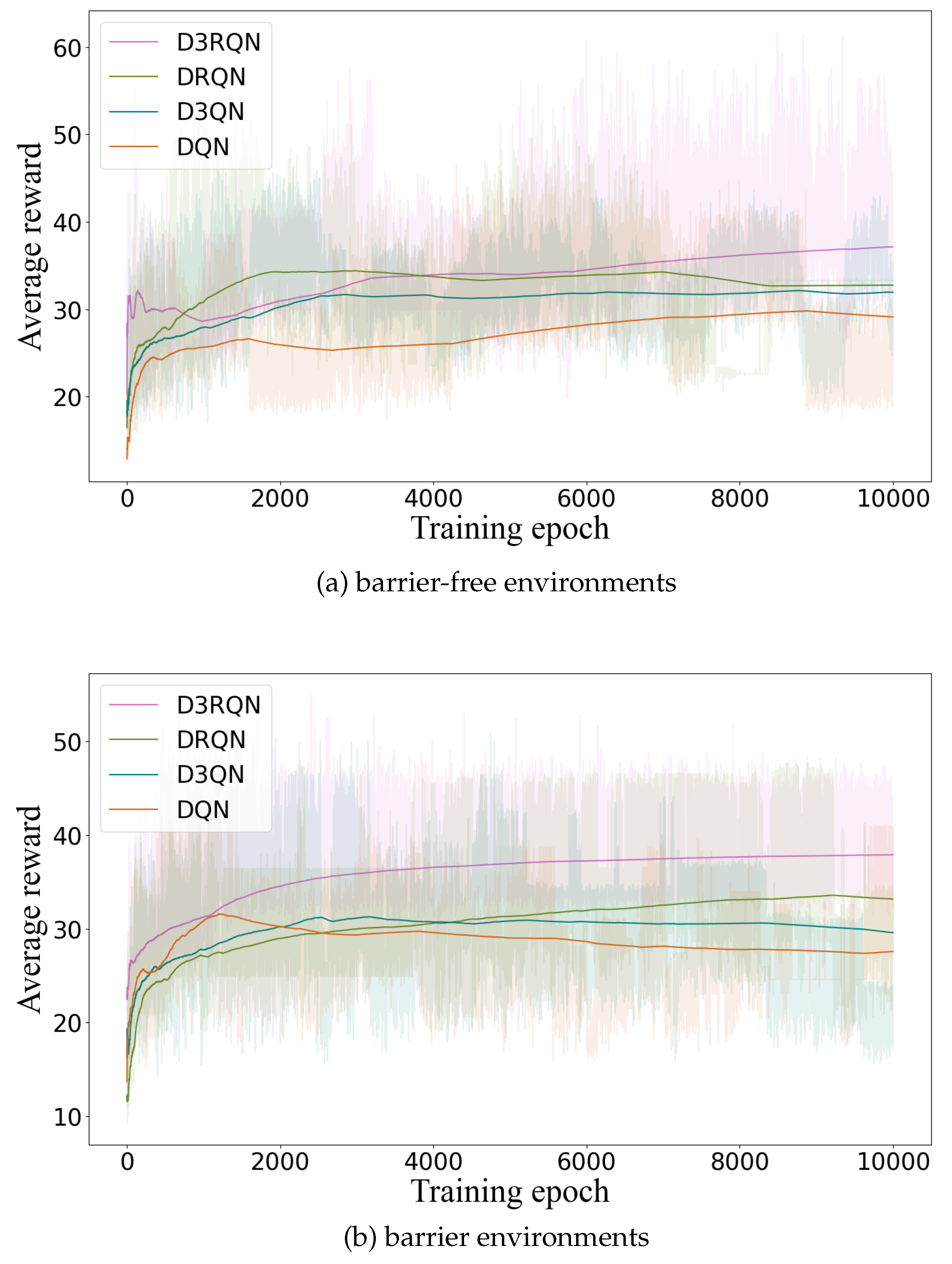
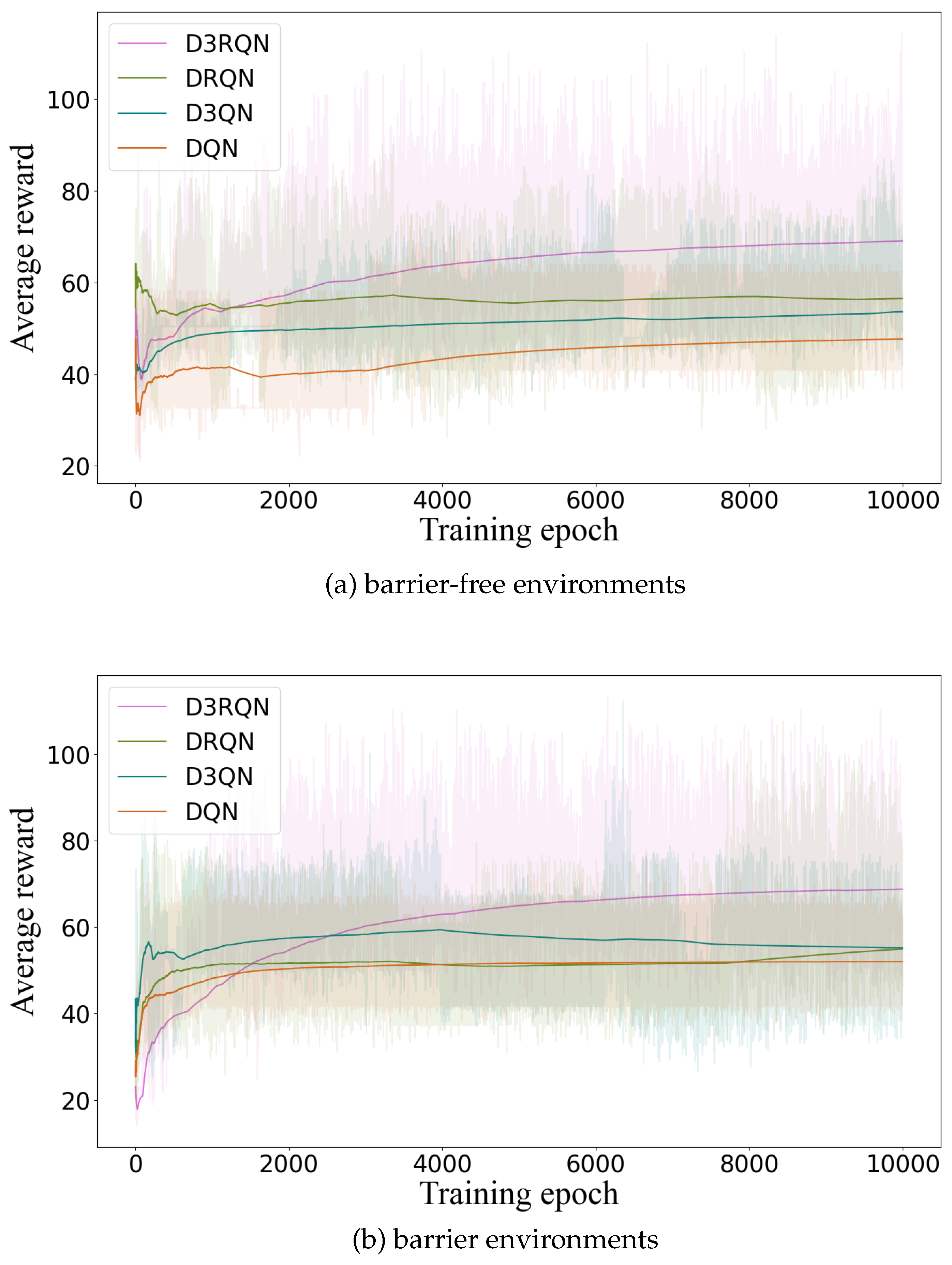
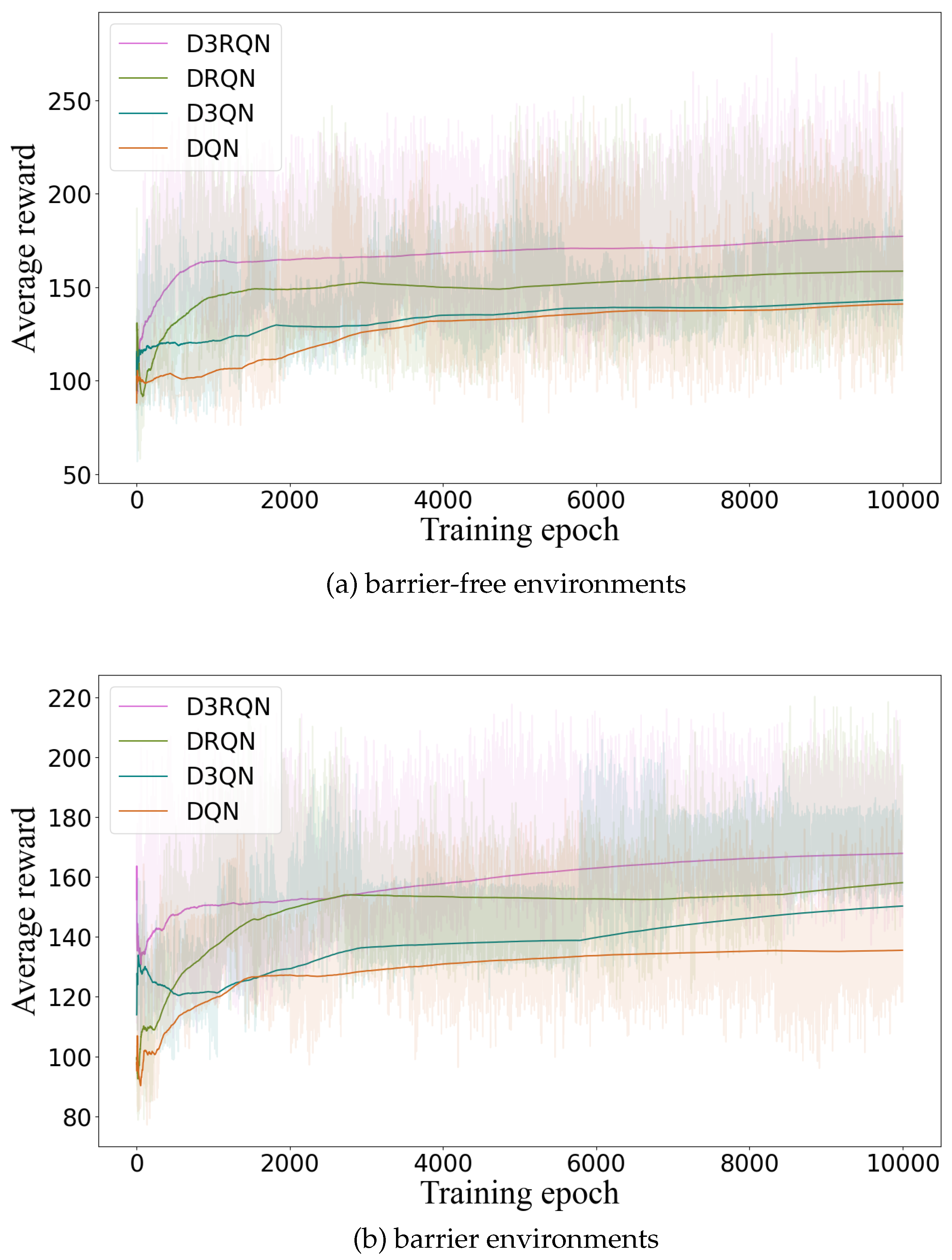
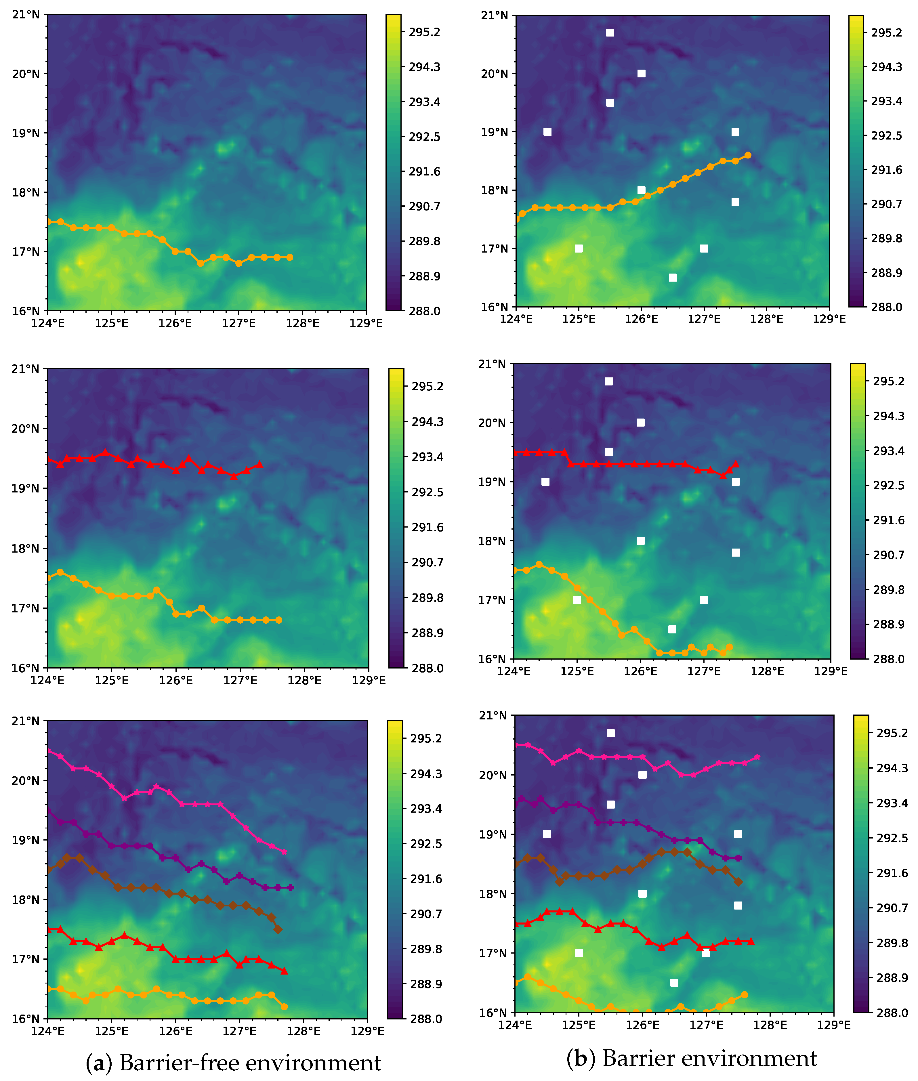
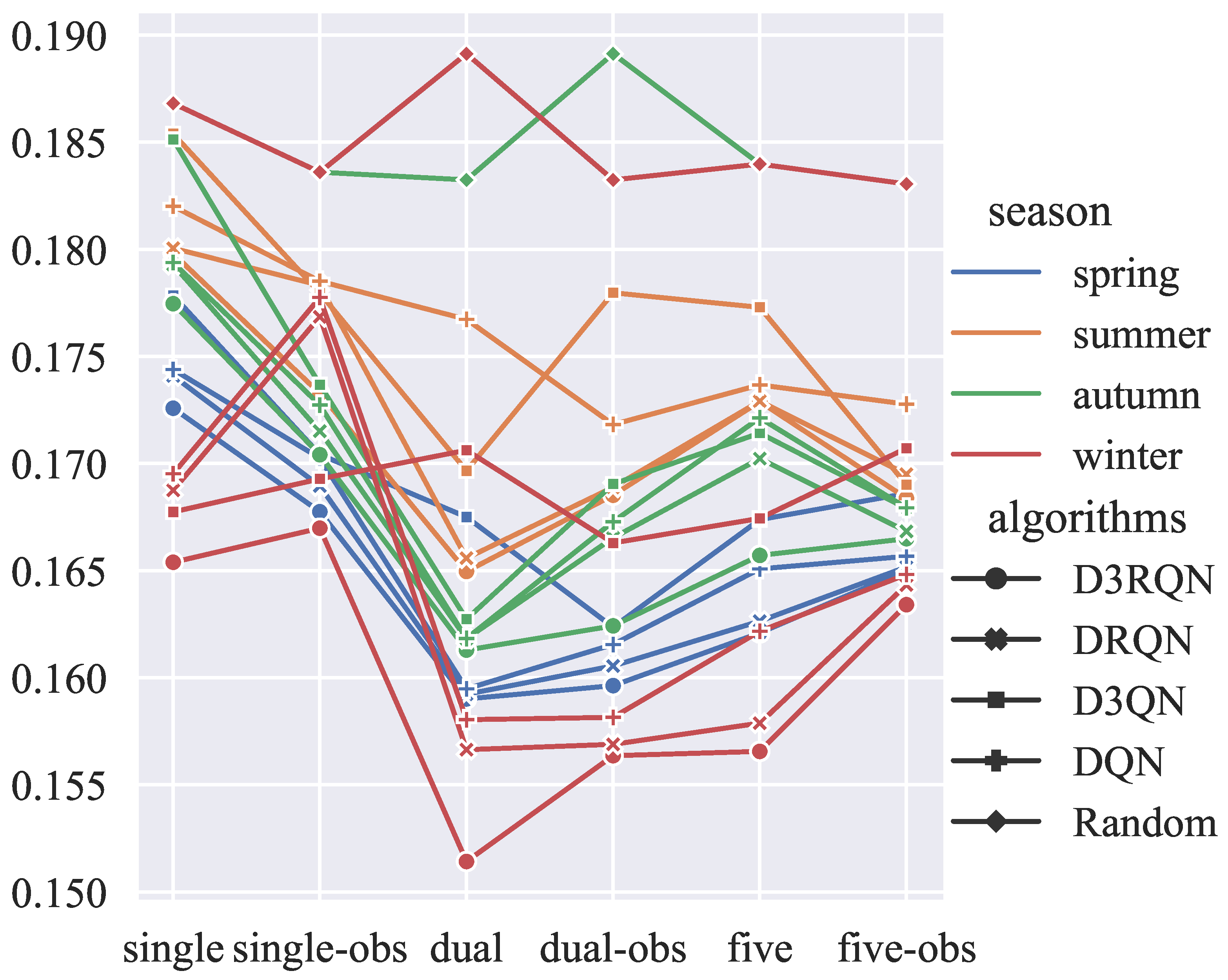
4.2. Observation Platform Sampling Results and Analysis

To order to verify the effectiveness of our algorithm, we conducted experiments in a barrier-free environment and a barrier environment. In each environment, we carried out single-platform, dual-platform and five-platform observation path experiments. Figure 5, Figure 6 and Figure 7 show the experimental results for the single platform, dual platforms, and five platforms, respectively.

Figure 5 shows the comparison of the experimental results of a single observation platform. In the comparison chart of the average reward function of a single mobile observation platform, the average reward value of the D3RQN algorithm is better than that of the other three algorithms. In the barrier-free environment, the D3RQN algorithm exhibits much exploration fluctuation at the beginning, but in the 300th to 3500th rounds, the DRQN algorithm is in the lead. When the number of rounds exceeds 4000, the D3RQN algorithm is in the lead until the end of training. However, the D3QN and DQN algorithms have low exploration efficiency and are at a disadvantage in the training process. In the barrier environment, after more than 1000 training iterations, the average reward of the D3RQN algorithm is always in the best position of the four algorithms.

Figure 6 shows the results of the dual platforms. In the comparison chart showing the average reward function of the dual mobile observation platform, the D3RQN algorithm is in the leading position among the four algorithms. In an barrier-free environment, the DRQN algorithm is superior in the first 1000 rounds of training. However, after more than 1000 rounds, the D3RQN algorithm is superior to the DRQ algorithm until the end of the training. When the number of rounds exceeds 4000, the D3RQN algorithm is in the lead until the end of training. The D3QN and DQN algorithms have low exploration efficiency and are at a disadvantage in the training process. Among them, DQN is always in the most inferior position. In a barrier environment, the D3RQN algorithm is in the most inferior state before 1500 rounds. When the number of rounds exceeds 1500, the DRQN and DQN algorithms succeed, and the D3QN algorithm succeeds for 2500 rounds, maintaining its advantages until the end of the training.

Figure 7 shows the comparison of the experimental results for five observation platforms. In the comparison chart showing the average reward function of the five observation platforms, the D3RQN algorithm is always in a dominant state in both environments. In an obstacle-free environment, the DRQN algorithm enters into a stable exploratory observation state for 1500 rounds until the end of the training. With obstacles, the D3RQN algorithm is in a relatively stable exploratory observation state after 2500 rounds.

Through the comparative analysis of the reward functions of the four algorithms in two environments, with the increase in the number of observation platforms, the D3RQN algorithm can maintain a stable exploratory observation state in the four algorithms. The DQN algorithm is always at the worst observation level. To sum up, the D3RQN algorithm with a cyclic convolution network can enable the observation platform to effectively observe the uncertain marine environment and obtain more effective observation information and data.

4.3. Assimilation Results and Analysis

To verify the influence of the sampling results of the observation platform on the quality of the forecast initialization, we assimilated the sampling results of the three algorithms on the three platforms. Figure 8 shows the sampling path of the observation platform based on the D3RQN algorithm. It can be seen from the figure that the observation platform can effectively avoid obstacles to sample places with large temperature differences.

We assimilate the environmental information collected by different algorithms in different environments. The results are shown in

Table 3. Spring: RMSE comparison of sampling and assimilation results of the observation path between a single platform and multiple platforms, RMSE${}_{raw}$ = 0.21733.

Platform	D3RQN	DRQN	D3QN	DQN	Random
$single$	0.17258	0.17409	0.17784	0.17439	0.18681
$singl{e}_{obs}$	0.16775	0.16895	0.17042	0.17025	0.18360
$dual$	0.15901	0.15923	0.16750	0.15948	0.18324
$dua{l}_{obs}$	0.15963	0.16055	0.16236	0.16155	0.18913
$five$	0.16209	0.16264	0.16738	0.16508	0.18398
$fiv{e}_{obs}$	0.16502	0.16517	0.16860	0.16567	0.18305

,

Table 4. Summer: RMSE comparison of sampling and assimilation results of the observation path between a single platform and multiple platforms, RMSE${}_{raw}$ = 0.21733.

Platform	D3RQN	DRQN	D3QN	DQN	Random
$single$	0.17980	0.18005	0.18539	0.18201	0.18681
$singl{e}_{obs}$	0.17327	0.17832	0.17796	0.17851	0.18360
$dual$	0.16496	0.16558	0.16966	0.17673	0.18324
$dua{l}_{obs}$	0.16852	0.16889	0.17797	0.17182	0.18913
$five$	0.17289	0.17291	0.17729	0.17367	0.18398
$fiv{e}_{obs}$	0.16838	0.16950	0.16901	0.17277	0.18305

,

Table 5. Autumn: RMSE comparison of sampling and assimilation results of the observation path between a single platform and multiple platforms.

Platform	D3RQN	DRQN	D3QN	DQN	Random
$single$	0.17746	0.17928	0.18513	0.17938	0.18681
$singl{e}_{obs}$	0.17041	0.17151	0.17368	0.17273	0.18360
$dual$	0.16129	0.16182	0.16273	0.16183	0.18324
$dua{l}_{obs}$	0.16242	0.16653	0.16904	0.16728	0.18913
$five$	0.16571	0.17023	0.17142	0.17213	0.18398
$fiv{e}_{obs}$	0.16649	0.16683	0.16790	0.16793	0.18305

and

Table 6. Winter: RMSE comparison of sampling and assimilation results of the observation path between a single platform and multiple platforms, RMSE${}_{raw}$ = 0.21733.

Platform	D3RQN	DRQN	D3QN	DQN	Random
$single$	0.16539	0.16875	0.16774	0.16952	0.18681
$singl{e}_{obs}$	0.16698	0.17685	0.16928	0.17775	0.18360
$dual$	0.15142	0.15664	0.17062	0.15804	0.18913
$dua{l}_{obs}$	0.15636	0.15689	0.16629	0.15815	0.18324
$five$	0.15656	0.15788	0.16744	0.16217	0.18398
$fiv{e}_{obs}$	0.16341	0.16433	0.17071	0.16482	0.18305

, and Figure 9.

It can be seen from Table 3, Table 4, Table 5 and Table 6, and Figure 9 that the RMSE of the assimilation results after the observation path planning of the mobile ocean observation platform is better than the RMSE of the background field data. The assimilation results based on the D3RQN algorithm are better than those of the DRQN, D3QN, and DQN algorithms. It can also be seen from Table 3, Table 4, Table 5 and Table 6, and Figure 9 that the assimilation results of the dual platform are better than the assimilation results of the single platform, but are not better than the assimilation results of the five platforms. This result shows that the quality of the assimilation results will increase with the increase in the number of samples. When the number of samples increases to a certain level, the quality of the assimilation results will not increase further.

5. Conclusions and Future Work

This research proposes a method for planning the observation paths of ocean mobile observation networks based on improved deep reinforcement learning algorithms. First, for the huge marine environment, we establish a partially observable Markov decision model, and develop a deep reinforcement learning framework for this complex and unknown environment. Due to the time-varying nature of the background field, the sampling process of the observation platform is affected by both the previous background field and the subsequent background field. In this regard, we add the bidirectional convolution network to the D3QN algorithm, and use the predictive ability of the bidirectional convolution network to make the observations of the previous state sequence and the subsequent state sequence close to the actual Q value, so as to improve the selection strategy for agents in the dynamic environment field. The simulation results show that our method can collect more marine environmental information than the DQN, D3QN, and DRQN algorithms. In addition, to improve the analysis accuracy of coupled environment elements and the quality of forecast initialization, we conducted observation experiments on a single platform, dual platform, and five platforms, and assimilated the experimental results. The assimilation results not only show that our observation program can improve the forecast quality, but also show that when the number of observation platforms reaches a certain number, adding more observation platforms will not improve the assimilation effect.

There is still much work to do in the future. First, we need to further study the effect of the proposed method in the continuous action space. Second, in addition to the temperature of the marine environment, we need to establish if there are other factors that play a role in improving the quality of marine forecast initialization.

References

1. Cai, S.Q.; Zhang, W.J.; Wang, S.A. An advance in marine environment observation technology. J. Trop. Oceanogr. 2007, 3, 76–81. [Google Scholar]
2. Wang, B.D. Autonomous Underwater Vehicle (auv) Path Planning and Adaptive On-Board Routing for Adaptive Rapid Environmental Assessment. Ph.D. Thesis, Massachusetts Institute of Technology, Cambridge, MA, USA, 2007. [Google Scholar]
3. Thomas, C.; James, B.; Josko, C.; Doug, W. Autonomous oceanographic sampling network. Oceanography 1993, 6, 86–94. [Google Scholar]
4. Bellingham, J.G.; Zhang, Y.; Godin, M.A. Autonomous Ocean Sampling Network-ii (aosn-ii): Integration and Demonstration of Observation and Modeling; Technical Report; Monterey Bay Aquarium Research Institute: Moss Landing, CA, USA, 2009. [Google Scholar]
5. Ramp, S.R.; Davis, R.E.; Leonard, N.E.; Shulman, I.; Chao, Y.; Robinson, A.R.; Marsden, J.; Lermusiaux, P.; Fratantoni, D.M.; Paduan, J.D. Preparing to predict: The second autonomous ocean sampling network (aosn-ii) experiment in the monterey bay. Deep Sea Res. Part II Top. Stud. Oceanogr. 2009, 56, 68–86. [Google Scholar] [CrossRef]
6. Barron, C.N.; Kara, A.B.; Martin, P.J.; Rhodes, R.C.; Smedstad, L.F. Formulation, implementation and examination of vertical coordinate choices in the global navy coastal ocean model (ncom). Ocean. Model. 2006, 11, 347–375. [Google Scholar] [CrossRef]
7. Robinson, A.R. Physical processes, field estimation and an approach to interdisciplinary ocean modeling. Earth-Sci. Rev. 1996, 40, 3–54. [Google Scholar] [CrossRef]
8. Lermusiaux, P. Adaptive modeling, adaptive data assimilation and adaptive sampling. Phys. D Nonlinear Phenom. 2007, 230, 172–196. [Google Scholar] [CrossRef]
9. Heaney, K.D.; Lermusiaux, P.; Duda, T.F.; Haley, P.J. Validation of genetic algorithm-based optimal sampling for ocean data assimilation. Ocean Dyn. 2016, 66, 1209–1229. [Google Scholar] [CrossRef] [Green Version]
10. Wang, C.-F.; Liu, K. A novel particle swarm optimization algorithm for global optimization. Comput. Intell. Neurosci. 2016, 2016, 48. [Google Scholar] [CrossRef] [Green Version]
11. Yilmaz, N.K.; Evangelinos, C.; Lermusiaux, P.; Patrikalakis, N.M. Path planning of autonomous underwater vehicles for adaptive sampling using mixed integer linear programming. IEEE J. Ocean. Eng. 2008, 33, 522–537. [Google Scholar] [CrossRef] [Green Version]
12. Heaney, K.D.; Gawarkiewicz, G.; Duda, T.F.; Lermusiaux, P. Nonlinear optimization of autonomous undersea vehicle sampling strategies for oceanographic data-assimilation. J. Field Robot. 2010, 24, 437–448. [Google Scholar] [CrossRef] [Green Version]
13. Lu, R.; Li, Y.C.; Li, Y.; Jiang, J.; Ding, Y. Multi-agent deep reinforcement learning based demand response for discrete manufacturing systems energy management. Appl. Energy 2020, 276, 115473. [Google Scholar] [CrossRef]
14. Mynuddin, M.; Gao, W. Distributed predictive cruise control based on reinforcement learning and validation on microscopic traffic simulation. IET Intell. Transp. Syst. 2020, 14, 270–277. [Google Scholar] [CrossRef]
15. Prrusquía, A.; Yu, W.; Li, X. Multi-agent reinforcement learning for redundant robot control in task-space. Int. J. Mach. Learn. Cybern. 2021, 12, 231–241. [Google Scholar] [CrossRef]
16. Gao, Y.; Yang, J.J.; Yang, M.; Li, Z. Deep reinforcement learning based optimal schedule for a battery swapping station considering uncertainties. IEEE Trans. Ind. Appl. 2020, 56, 5775–5784. [Google Scholar] [CrossRef]
17. Yang, Y.; Vamvoudakis, K.G.; Modares, H. Safe reinforcement learning for dynamical games. Int. J. Robust Nonlinear Control 2020, 30, 3706–3726. [Google Scholar] [CrossRef]
18. Yan, C.; Xiang, X.; Wang, C. Towards real-time path planning through deep reinforcement learning for a uav in dynamic environments. J. Intell. Robot. Syst. 2020, 98, 297–309. [Google Scholar] [CrossRef]
19. Wen, S.; Zhao, Y.; Yuan, X.; Wang, Z.; Manfredi, L. Path planning for active slam based on deep reinforcement learning under unknown environments. Intell. Serv. Robot. 2020, 13, 263–272. [Google Scholar] [CrossRef]
20. Yao, Q.; Zheng, Z.; Qi, L.; Yuan, H.T.; Yang, T. Path planning method with improved artificial potential field—A reinforcement learning perspective. IEEE Access 2020, 8, 135513–135523. [Google Scholar] [CrossRef]
21. Li, B.; Wu, Y. Path planning for uav ground target tracking via deep reinforcement learning. IEEE Access 2020, 8, 29064–29074. [Google Scholar] [CrossRef]
22. Jiang, J.; Zeng, X.; Guzzetti, D.; You, Y. Path planning for asteroid hopping rovers with pre-trained deep reinforcement learning architectures. Acta Astronaut. 2020, 171, 265–279. [Google Scholar] [CrossRef]
23. Wang, B.; Liu, Z.; Li, Q.; Prorok, A. Mobile robot path planning in dynamic environments through globally guided reinforcement learning. IEEE Robot. Autom. Lett. 2020, 5, 6932–6939. [Google Scholar] [CrossRef]
24. Wei, Y.; Zheng, R. Informative path planning for mobile sensing with reinforcement learning. In Proceedings of the IEEE INFOCOM 2020—IEEE Conference on Computer Communications, Toronto, ON, Canada, 6–9 July 2020. [Google Scholar]
25. Josef, S.; Degani, A. Deep reinforcement learning for safe local planning of a ground vehicle in unknown rough terrain. IEEE Robot. Autom. Lett. 2020, 5, 6748–6755. [Google Scholar] [CrossRef]
26. Shchepetkin, A.F.; Mcwilliams, J.C. The regional oceanic modeling system (roms): A split-explicit, free-surface, topography-following-coordinate oceanic model. Ocean. Model. 2005, 9, 347–404. [Google Scholar] [CrossRef]
27. Summerhayes, C. Technical tools for regional seas management: The role of the global ocean observing system (goos). Ocean Coast. Manag. 2002, 45, 777–796. [Google Scholar] [CrossRef]
28. Surhone, L.M.; Tennoe, M.T.; Henssonow, S.F. Partially Observable Markov Decision Process. 2010. Available online: https://www.morebooks.de/shop-ui/shop/product/978-613-1-26000-1 (accessed on 15 November 2022).
29. Ragi, S.; Chong, E.K.P. Uav path planning in a dynamic environment via partially observable markov decision process. IEEE Trans. Aerosp. Electron. Syst. 2013, 49, 2397–2412. [Google Scholar] [CrossRef]
30. Sutton, R.; Barto, A. Reinforcement Learning: An Introduction; MIT Press: Cambridge, MA, USA, 1998; Volume 9, p. 1054. [Google Scholar]
31. Hasselt, H.V.; Guez, A.; Silver, D. Deep reinforcement learning with double q-learning. Comput. Sci. 2016, 30. [Google Scholar] [CrossRef]
32. Mnih, V.; Kavukcuoglu, K.; Silver, D.; Rusu, A.A.; Veness, J.; Bellemare, M.G.; Graves, A.; Riedmiller, M.; Fidjeland, A.K.; Ostrovski, G.; et al. Human-level control through deep reinforcement learning. Nature 2015, 518, 529–533. [Google Scholar] [CrossRef]
33. Wang, Z.; Freitas, N.D.; Lanctot, M. Dueling network architectures for deep reinforcement learning. In Proceedings of the 33rd International Conference on Machine Learning (ICML 2016), New York, NY, USA, 19–24 June 2016. [Google Scholar]
34. Hausknecht, M.; Stone, P. Deep recurrent q-learning for partially observable mdps. Comput. Sci. 2015, arXiv:1507.06527. [Google Scholar] [CrossRef]
35. Wang, X.; Gursoy, M.C.; Erpek, T.; Sagduyu, Y.E. Learning-based uav path planning for data collection with integrated collision avoidance. IEEE Internet Things J. 2022, 9, 16663–16676. [Google Scholar] [CrossRef]
36. Jahrer, Preparing Continuous Features for Neural Networks with Gaussrank. Available online: http://fastml.com/preparing-continuous-features-for-neural-networks-with-rankgauss/ (accessed on 22 January 2018).
Figure 1. A USV motion coordinate system.
Jmse 11 00208 g001
Figure 2. Adaptive observation based on D3RQN.
Jmse 11 00208 g002
Figure 3. Proposed D3RQN structure with bidirectional recurrency.
Jmse 11 00208 g003
Figure 4. Data processing.
Jmse 11 00208 g004
Figure 5. Comparison of the experimental results of a single observation platform. (a,b) Comparison of the reward functions of DQN, D3QN, DRQN, and D3RQN running in barrier and barrier-free environments, respectively.
Jmse 11 00208 g005
Figure 6. Comparison of the experimental results of dual observation platforms. (a,b) Comparison of the reward functions of DQN, D3QN, DRQN, and D3RQN running in barrier and barrier-free environments, respectively.
Jmse 11 00208 g006
Figure 7. Comparison of the experimental results of five observation platforms. (a,b) Comparison of the reward functions of DQN, DRQN, D3QN, and D3RQN running in barrier and barrier-free environments, respectively.
Jmse 11 00208 g007
Figure 8. Observation platform sampling path.
Jmse 11 00208 g008
Figure 9. RMSE comparison chart of different algorithms in four seasons.
Jmse 11 00208 g009