The Management of the Beach-Cast Seagrass Wracks—A Numerical Modelling Approach

Abstract

Seagrass wrack are commonly found on the beach face of the sandy shore all around the world and often persists in situ during the whole year, favouring the emergence of conflicts for the use of the sandy coasts for bathing or for other recreational purposes. As a consequence, these deposits are often removed from the beach during the summer months, temporary stocked, and relocated on the shore face in the next autumn or winter season. The selection of the sites on the shoreline where the leaves should be released before the storms season is often an issue, considering the optimization needs between the transportation costs and the oceanographic features of the dumping site. In this study, a numerical approach was proposed to identify the most suitable areas for the autumnal repositioning of the seagrass wracks for two beaches of Sardinia, an island located in the Western Mediterranean Sea where Posidonia oceanica (L. Delile, 1813) is the most widespread seagrass species. The method is based on the use of hydrodynamic, wave, and particle tracking models and provides important indications useful for the management of this type of practice that can be extended to all different type of beaches along the Mediterranean coasts.

1. Introduction

Seagrass wrack, detached leaves, and stems are commonly found on beaches all around the world [1,2,3,4] and their deposition occurs on the beach face of the sandy shore [5]. Posidonia oceanica (L. Delile, 1813) is the most widespread seagrass species of the Mediterranean Sea [6] forming large meadows that colonize the sea bottom up to a depth of 40 m [7]. It is a multiannual marine plant with a maturation cycle of the leaf apparatus characterized by a continuous growth with detachments during the autumn and regrowth during the winter periods. As a consequence, in those traits of coasts facing P. oceanica meadows, the detachments and regrowing processes can produce accumulation of the leaves on the shore. In particular, since the leaves are characterized by negative buoyancy, their accumulation on the shore is mainly due to the direct action of the wind waves and of the wave-induced littoral currents.

On sandy shores, the cast litter of P. oceanica leaves transported by the waves and currents can generate wedge structures defined as “banquettes” [8]. The presence of these deposits along the shores, mostly observed during the winter and autumn, are found mainly in the beach face [4,5]. Similar to sediment berms, the seagrass banquettes are generated by the accumulation of seagrass litter and sediments at the extreme landward edge of the wave influence [9]. Banquettes are not only composed of vegetal material (e.g., roots and leaves), in fact, up to 100 kg m⁻³ of sediments can be found trapped inside [5,10] therefore contributing to the sedimentary budget of the beaches.

The P. oceanica beach cast litter influences also to the beach morphology [3], being layers of P. oceanica leaves frequently found trapped inside the morphological structures of the backshore as the berms and the beach ridges. Furthermore, the P. oceanica beach cast litter can provide nutrients for the incipient foredune in terms of leaves and parts of plant pushed by wind and trapped by pioneer plants [11].

Beach-cast vegetation litter is harvested for biomass exploitation [1] and to improve the recreational use of beaches for tourism [2] in various coastal areas all around the world. These accumulations often persist in situ during the winter period and, in some cases, during the whole year, favouring the emergence of conflicts for the use of the sandy coasts for bathing or for other recreational purposes [4].

As a consequence, P. oceanica banquettes are often removed from the shore in order to favour the use of the beach for touristic activities [12]. These removal procedures are commonly carried out in several beaches in the Mediterranean Sea [4,13,14]. As an example, in Sardinia, an Italian island located in the Western Mediterranean, during the 2004, about 106,000 m³ of banquettes have been removed from 114 km of beaches, mainly by using heavy machinery [4].

Among the Mediterranean areas where P. oceanica meadows exist, the Sardinian coastal waters represent those littorals where the conflicts between the presence of banquettes and the recreational usage of sandy shores are intense. As a consequence, the local regional authorities issued specific regulations and practices to manage the P. oceanica beach-casts. In particular, in this region, a specific framework provides recommendations for the management of the banquette [15], which removal is allowed under a series of specific guidelines that should be applied by the coastal Municipalities. In particular, the movement of the banquettes from the beach face is permitted only during specific periods of the year, with specific mechanical means and only if delivered into a stocking area located on the same beach. This practice must be carried out before the early summer with the recommendation of repositioning the removed amount of banquettes in the beach face before the next winter season, to guarantee the return of the biomass into the sea and provide further protection against the winter storms.

The selection of the site on the shore face where releasing the leaves in late autumn before the storms season is often an issue, considering the optimization needs between the transportation costs and the oceanographic features of the dumping site. The transport of the banquette depends on several factors as the accessibility of the beach, the location of the stocking area, and the type of vehicle used, with the consequence that a standardized procedure cannot be easily assessed. On the other hand, the choice of the dumping site in relation to its environmental features can be addressed by following standardized methods. In particular, the selection should consider the local oceanographic conditions favouring those sites where the waves and currents promote an efficient transport of the leaves far from the released area. This criterion follows both the necessity to avoid multi-year accumulation, which would increase the beach cast management costs and the will of preserving the nutrient budgets in the local coastal waters by releasing the P. oceanica leaves previously removed.

At present time no studies were realized to optimize the efficiency of the reallocation of the banquette in the shore face by promoting their dispersion by waves and currents, with the consequence that the coastal managers localize the better reposition site on the basis of random and subjective choice. In our study, for the first time we investigate the hydrodynamic features of sites along the beaches where the banquette could be repositioned in order to identify those areas guaranteeing an efficient dispersion of the leaves.

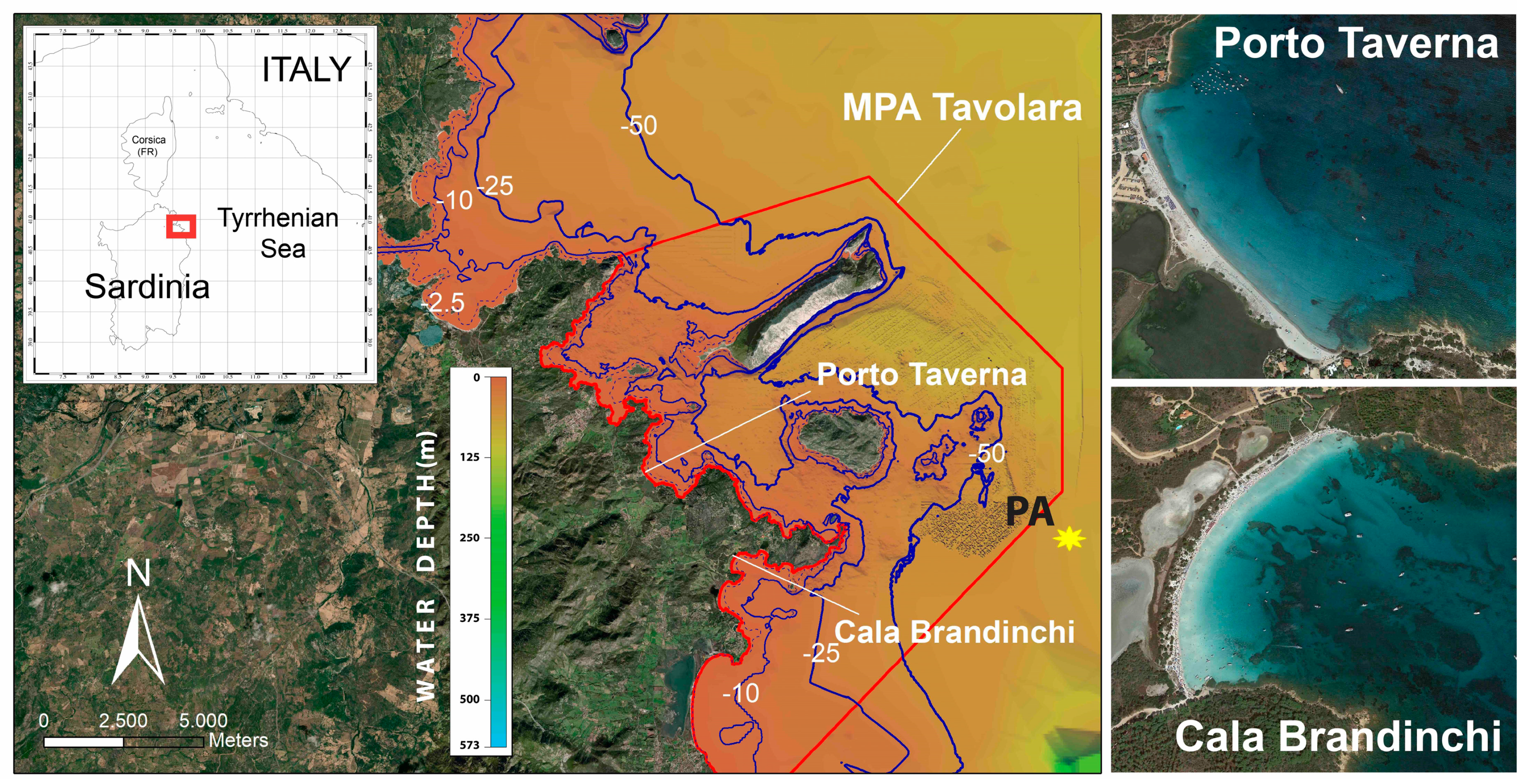
With these premises, this study aims to identify the most suitable areas for autumnal repositioning of the P. oceanica leaves for two beaches, Porto Taverna (PT) and Cala Brandinchi (CB; see Figure 1), located within the marine protected area (MPA) of Tavolara Punta Coda Cavallo, along the eastern coast of Sardinia Island. The MPA was established on the 12th December 1997 by the Italian Ministry of Environment and extends for a total surface of 15,280 ha, including several coastal marine habitats with P. oceanica meadows, rocky outcrops, coralligenous assemblages and sandy muddy bottom mainly characterizing the MPA seabed [16]. Coastal geomorphology is characterized by granite of Ercinic origin with several sandy beaches, including pocket beaches, enclosed in the MPA [17].

The two beaches, PT and CB, extending for around 800 and 600 m length and facing the Tyrrhenian Sea, were selected both for their exposition to the prevalent wind and wave regimes of the area and for the presence of large P. oceanica meadows in front of the two littorals and for the intense recreational usages during the summer months, which turns into conflict with the accumulation of a banquette on the shore face. PT and CB can be classified as pocket beaches and represent the typical geomorphological units characterizing the sandy traits of this MPA coastline [16]. The sediments grain size of PT varies between coarse to medium sand, whereas the sediments of CB are mainly composed of fine sand.

In both sites, every year, less than 100 m³ of beach-casts mostly made of P. oceanica leaves are manually removed at the beginning of the summer touristic season to be temporarily stocked behind the foredune and to be put again on the foreshore in the next late autumn. Up to now, the selection of the dumping sites on the shoreline is done considering only the logistic aspects without any evaluation on the oceanographic conditions characterizing the two study sites.

For both study cases, a numerical approach was followed applying high resolution coupled wave hydrodynamic and particle tracking models to reproduce the main physical processes ruling the dispersion of the P. oceanica leaves into the seawaters. Numerical simulations were carried out considering the main meteo-marine forcing in the area of investigation and the results were processed to indicate the optimal location along the two shores that can promote the transport of the leaves far from the two beaches.

The paper is organized as follow: in Section 2 the collection of environmental data, the adopted numerical methods, and the simulation setup were described; in Section 3 the model results were reported including the description of the wave and current dynamics characterizing the two coastal areas and of the P. oceanica leaves transport simulations results; and, finally, the results were discussed, and the conclusions drawn.

2. Materials and Methods

2.1. Environmental Records

Geomorphological properties and meteorological and marine prevalent conditions were defined through a collection of experimental and modelling records, with the intent of adequately setting up the numerical model applications.

2.1.1. Morphological Data

The collection and analysis of highly detailed bathymetric and cartographic data are a necessary and preliminary step to the application of hydrodynamic and wave numerical models in the investigation area. For both study sites, ad-hoc bathymetric surveys were carried out to collect high-resolution depth and elevation data in the submerged and the emerged part of the beach, respectively. Specifically, single-beam echo sounder was used to map the sea-bed along preselected profiles (see Figure 2) and covering the area in between the isobath of 10 and 0.5 m for the PT, and between the isobath of 15 and 0.5 m for the CB. The instrument was installed on a leisure boat and linked to a differential GPS in order to ensure an accuracy of 10 cm on both depth and position measurements.

Those tracks that were perpendicular to the shoreline were taken as references for the sampling of the beach slope, from the 0.5 m depth up to the berm position, on the emerged part of the beach. A differential GPS mounted on a stick was used to define the elevation of the beach profile.

The entire set of the collected data was then processed and interpolated on a regular mesh with a cell size of 20 m, to obtain a digital terrain elevation model (DTM) of the beaches and of the sea-bottom of the bays. For the offshore part of the domain, the bathymetric data were derived from the digitalization of nautical charts and from the General Bathymetric Chart of the Oceans dataset (GEBCO) [18]. In Figure 1 the DTM is reported for the extended area comprising of the PT and CB bays and the whole MPA of Tavolara Punta Coda Cavallo.

The elevation data collected along each emerged track were processed to compute the slope of the shoreline from the 0.4 m depth up to the berm position. The slopes were similar along both shores being characterized by low standard deviation values estimated around 2, therefore, the average beach slopes were computed obtaining 7% and 8%, for the PT and BC sites, respectively.

2.1.2. Meteo-Marine Data

The typical wave regimes characterizing the study sites were analysed in terms of incident wave energy, direction, and number of events in order to individuate a satisfactory number of scenarios that could characterize the local wave climate. Specifically, the authors selected an eleven-year period (2007–2017) of wave data that were produced at hourly frequency by the back-testing of the Mediterranean Waves Forecasting System [19], released by the EU ocean data provider Copernicus (see https://marine.copernicus.eu for further information) and collected at 40.843462° E and 9.809011° N, a point located offshore both the study sites (see PA in Figure 1). In Figure 3, panel A, a scatter plot describes the relation between the significant wave height (SWH) and the wave direction (D) for the whole set of data.

Qualitatively, the highly energetic events, indicating the storms, distribute mainly between the first (N-NE) and the second quarter (E-SE) corresponding to the typical direction of the Grecale and Sirocco winds [20]. Maxima of SWH, up to 7 m and 6 m, were found in the correspondence of such two directions whereas lower values, between 1 and 2 m, were found in the correspondence of the other directions. The peak located at NW is generated by the Mistral wind, one of the main anemometric regimes in the area, which is directed offshore and was not capable of generating intense storm events at the coast.

Considering the period of the year when the P. oceanica leaves dumping practice occurs, between the autumnal and the winter season, a quantitative analysis of the wave energy distribution along the directions was carried out for this part of the year only. In Figure 3, panel B, the polar graph of the frequency distributions of the main wave energy classes as a function of the wave direction is shown. The wind notation for direction was adopted also for the wave therefore, a wave directed to north is indicated by its provenience, which is the south. The three main wave and related wind regimes from N-NE (Grecale), from NW (Mistral), and from S-SE (Sirocco) are clearly recognizable in the polar plot, with the 28% of the events from N-NE, 27% from NW, and 26% from S-SE, respectively. Most of the events, about 48%, were characterized by SWH lower than 1 m. The maxima of the wave heights were observed from the 1st quadrant with several events with SWH higher than 5 m. The Sirocco regime was characterized by moderate storms, with wave height peaks generally lower than 3 m heights, whereas the Mistral regime, even if contributing to the wave energy budget in the selected location with low to moderate intensities, was not affecting the wave climate of the two coastal study sites due to its propagation direction.

The wave data were statistically analysed in Section 3.1 in order to identify the main meteo-marine scenarios that more frequently affect the two coastal sites and promote a local circulation capable to transport and disperse the P. oceanica leaves offshore.

2.2. Numerical Methods

The transport of the seagrass wracks at sea was investigated following a numerical modelling approach based on the use of hydrodynamic, wave, and particle tracking models.

Specifically, a high-resolution three-dimensional ocean model, based on the finite element method, shallow water hydrodynamic finite element model (SHYFEM) [21], was adopted to reproduce the wind and waves induced water circulation in the two study sites. SHYFEM is an open source-ocean model software [22], which resolves the 3-D shallow water equations vertically integrated over z-layers, accounting for meteorological and ocean forcing including wind, thermal fluxes, tides, and thermohaline contribution to the fluid flow.

In order to account for the wave effects, SHYFEM is online coupled with a spectral wave model named Wind Wave Model (WWM) [23]) that solves the wave action equation system (WAE) using the finite element method to predict the generation, propagation, and dissipation of the wind waves. The two models exchange, at each computational time step and on the same model mesh, the necessary information to reproduce the wave–current interaction and its effects on the littoral circulation.

The hydrodynamic and wave fields predicted by SHYFEM–WWM were used as input data by an offline particle tracking model (PTM) [24] to simulate the seagrass wrack transport and deposition processes. In the Appendix A, a detailed description of the numerical methods and equations system is reported.

This numerical framework has been already applied with success in previous studies to simulate the hydro and waves dynamics and the related transport processes in both open and coastal waters of the Mediterranean Sea [20,25,26,27,28,29,30].

2.2.1. Hydro-Wave Model Simulation Setup

SHYFEM uses a semi-implicit algorithm for the temporal integration and finite elements methods based on unstructured meshes for the spatial integration of the momentum and continuity equation system.

Two different meshes were implemented to reproduce the morphological features of the two study sites. Both meshes are constituted by about 95,000 triangular elements with a total of about 50,000 computational nodes. The size and shape of the elements vary in space with higher densities in the proximity of the PT and CB bays, where spatial resolution up to 10 m was imposed.

The model domains extend to the whole Tyrrhenian Sea and part of the Sicily Channel with an increment of the spatial resolution in correspondence of the fetches of the main wind regimes of the area. This computational approach accounts for all the surfaces contributing to the generation and propagation of the wind waves in the region of interest and permits to set the perimeter of the whole model domain as a closed boundary. The bathymetric details were reproduced by integrating the high-resolution depth data, described in Section 2.1.1, with the large-scale GEBCO dataset [18]. In Figure 4 the two finite element meshes are depicted along with the bathymetric information at different magnification levels. In both cases, the model domain extended onshore up to the coastline, which constitutes a closed boundary for the model simulation. Vertical direction was discretized by means of 20 uneven z-levels with the intervals between layers varying from 0.5 m, for the surface, up to 500 m for the last layer and with the first 10 m depth discretized by 11 layers.

The astronomic tides in the area are very weak and tidal-induced water circulation can be neglected [29]. The absence of fresh water inputs in the area and the shallow marine environment led to excluding the thermohaline contribution to the motion in the two areas [29]. Therefore, the wind and the wave can be considered as the main forcing promoting the water circulation in the two study sites.

For the wave scenarios that will be defined in Section 3.1, consisting of a set of wave heights and directions representing the local wave climate, WWM was applied in the 1-D mode along the fetch characterizing each specific wave regime. This allows estimating the intensity of the steady wind generating the desired SWH. A trial and error method was then used to estimate, for each wave scenario, the corresponding wind forcing (wind speed and direction). The obtained data will constitute the surface boundary conditions for a series of fully 3D coupled wave–current simulations carried out for the duration of 3 days. During this time interval, the wind increased linearly to its maximum after the first day, which roughly corresponds to the typical lifetime of the cyclogenesis in the Central Mediterranean Sea [31,32], to decrease to 0 during the next 2 days of simulation. A dynamical time stepping procedure was followed with a Courant threshold equal to 0.5. For each scenario and study site, the water circulation in the three dimensions and the distribution of the significant wave height (SWH), wave period (T), and direction (D) were computed for the whole duration of each run.

2.2.2. PTM Setup

Hydrodynamics and wave model data were used as input by the offline coupled PTM to simulate the dispersion of the P. oceanica (PO, hereafter) leaves released on the shorelines of the two study sites.

Five main dynamical processes ruling the transport of the banquettes from the shoreline to the sea were considered: immersion, transport, deposition, resuspension, and stranding. The immersion of the PO leaves occurs when the wave run-up reaches the banquettes on the shoreline. The dry leaves are then transported at the surface by the water currents until the beginning of sinking, which occurs after the wetting process is completed. At the bottom, the PO is deposed until the shear stress threshold for the resuspension is overcome by the wave and current action. The wet PO is therefore carried again by the vertically averaged water circulation up to a new deposition occurs. The PO stranding is promoted by the wave breaking and acts on both the wet and dry phases of the leaves transport at sea.

These processes were simulated combining the Eulerian information, provided at each computational time step by the hydrodynamic and wave model, and the Lagrangian paths followed by numerical particles emulating the PO leaves.

Specifically, the PTM described in the Appendix A was used to simulate the main dynamical processes ruling the transport of the PO leaves at sea. For each simulation, numerical particles were released continuously in the mesh boundary elements constituting the shoreline of the two beaches. At each computational time-step, the runup of the incident waves on the foreshore was computed following the Stockdon formula [33], which reads as:

$$\begin{gathered} \mathrm{R}=1.1\left(0.35\mathsf{\beta }\sqrt{\mathrm{SWH}\ast \mathrm{T}}+\frac{\sqrt{\mathrm{SWH}\ast \mathrm{T}\left(0.563{\mathsf{\beta }}^2+0.004\right)}}{2}\right) \\ \mathrm{DM}=\frac{\mathrm{R}}{\sin ({\tan }^{-1}\mathsf{\beta })} \end{gathered}$$

(1)

with$\mathsf{\beta }$ the beach slope obtained from experimental data in Section 2.1.1, SWH and T the computed wave height and period in front of the shore, R the height of the runup, and DM the distance from the shoreline reached by the incident wave.

For DM values higher than 2 m, the immersion process is activated, and the transport of the numerical particles starts. This threshold was defined considering the positioning of banquettes generally within the first 2 m from the shoreline and assuming only the waves surmounting the whole deposit as capable to drag the leaves into the waters. The leaves immersion is simulated only for the growing phase of the storm scenario when the wave energy is increasing in time.

In accordance with [34], which empirically estimated the leaves wetting timescale, the surface transport of the dry leaves occurred only for the first 7300 s from their immersion. During this dry phase, the transport of the numerical particles was simulated by solving Equation (A3) in Appendix A, using the computed surface current components for ${\mathrm{u}}_{\mathrm{a}}$ and ${\mathrm{v}}_{\mathrm{a}}$ and setting the inertial factors ${\mathsf{\alpha }}_c$ and ${\mathsf{\alpha }}_w$ equal to 0.7, as suggested by [34]. A similar approach was followed for the turbulence velocities ${\mathrm{u}}_{\mathrm{d}}$ and ${\mathrm{v}}_{\mathrm{d}}$ computed through random walk techniques and scaled by a factor of 0.7. At the end of the dry phase the leaves sink with a settling velocity of 0.15 m/s as estimated by [34]. The PTM simulates the vertical displacement of the numerical particles up to the sea bottom where the particles deposit. During the sinking, or wet phase, the horizontal displacement is computed using, as inputs, the vertically averaged current velocities and weighting the Stokes drift contribution with a factor inversely correlated to the particle depth. Once at the seabed, the leaves can be resuspended, and the particles transported in the wet phase again. The resuspension occurs only when the computed bottom shear stress induced by the waves and currents are higher then $8\times {10}^{-5}$ N/m², as suggested by [34]. Finally, when the numerical particles were carried over the model boundaries, consisting in the shoreline, the leaves were considered as stranded.

During the simulation, at each time step and, for each sedimented particle, the distance from the beach shoreline was computed and associated with the initial particle position on the shore. Subsequently, for each shoreline element, the average distance travelled by the released particles was calculated and mapped. This quantity was normalized and defined as the relative dispersion index (RDI).

3. Results

In the following, the results obtained by the analysis of the meteo-marine data aimed to define the simulation scenarios and the results obtained by the numerical model applications were reported. The section was organized as follows, in the first part the available wave data were analysed to define the wind intensity and direction characterizing the main meteo-marine scenarios, in the second part the wave propagation and the induced water circulation in the two study sites obtained for each simulated scenario were presented, then, in the third part, the results obtained by the simulation of the PO leaves transport were reported.

3.1. Analysis of the Wave Records

In

Table 1. Eleven years waves statistics at location 40.843462° E, 9.809011° N. Number of events (Oc) with SWH higher then 1 m for each 30° sector of wave provenience (Sect); average SWH (AH), average of the seasonal maxima SWH (AM), and absolute maximum SWH (MH).

AUTUMN-WINTER
Sectors	Oc	AH (m)	AM (m)	MH (m)
0–30°	5659	1.6	3.7	7.1
30–60°	2051	1.3	3.2	4.5
60–90°	1160	1.2	2.2	4.5
90–120°	1540	1.2	2.5	5.7
120–150°	5620	1.2	2.9	6.3
150–180°	3855	1.0	2.2	3.8
180–210°	438	0.8	1.2	1.7
210–240°	278	0.8	1.2	1.8
240–270°	387	0.9	1.3	1.8
270–300°	1208	0.9	1.4	2
300–330°	5373	1.1	2.3	2.9
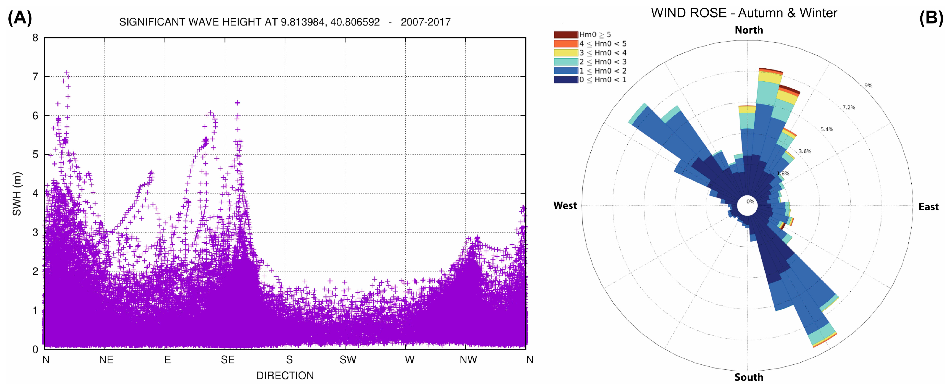
330–360°	1996	1.0	2.5	3.6

, the statistics of the eleven-years wave dataset was reported for the winter and autumn period. The data were preliminary filtered considering only the wave events higher than 1 m and therefore excluding lower values generated by breeze events or by low intensity meteorological instabilities. The results highlight and confirm how the main regimes of the local wave climate, between 0 and 60° and between 120 and 180°, correspond to the Grecale and to the Sirocco wind provenience directions. For both regimes, the average SWH (AH in Table 1) varied between 1 and 1.6 m with higher values for the northern sectors. Significant differences were found between the averages of the yearly maximum SWH (AM in Table 1) with the highest values of 3.7 m for the Grecale and 2.9 m for the Sirocco regime. Finally, the highest energetic events during the whole eleven-years period (MH in Table 1) occurred in the selected seasons with maximum SWH of 7.1 m for the Grecale and of 6.3 m for the Sirocco regime, respectively.

The previous analysis provides indications that the wave climate of the two coastal sites can be represented by two main directions, corresponding to the provenience direction of Grecale and Sirocco winds, and by two energetic levels, obtained by averaging the AH values, for the lower energetic case, and the AM values for the higher energetic case.

Four different scenarios can be then obtained (see

Table 2. Wave scenarios. The four different scenarios characterizing the wave climate in the two study sites with directions and SWH reported.

Scen.	Dir.	SWH (m)
ST_G1	30°	1.5
ST_G2		3.5
ST_S1	150°	1.2
ST_S2		2.5

), with wave directions corresponding to 30°, Grecale directions, and 150°, Sirocco direction, and with wave heights varying between 1.5 and 3.5 m for the first case and between 1.2 and 2.5 m for the second case.

These values represent the wave conditions that more frequently affects the two coastal sites and that, due to their moderate or high intensity, can promote a local circulation that is capable to transport and disperse the P. oceanica leaves offshore. The highest events were not considered being infrequent and therefore not suitable as a benchmark for testing the dumping procedure.

For each wave scenario described in Table 2, following the method described in Section 2.2.1, the steady wind intensity, generating the corresponding SWH, was computed obtaining speeds of 9 m/s for the scenario ST_G1, 14 m/s for the ST_G2, 8 m/s for the ST_S1, and 11 m/s for ST_S2, which are representative of the typical moderate and intense storm events in the area [29,35]. These data constituted the surface boundary conditions for four fully 3D coupled wave–current simulations carried out for each study site for the duration of 3 days as detailed in Section 2.2.1.

3.2. Modelled Wave and Currents

The model was applied to reproduce the wave and currents fields in the two study sites for the four different meteo-marine scenarios described in Table 2, two for Grecale (ST_G1 and ST_G2), and two for Sirocco wind regimes (ST_S1 and ST_ S2). For all the cases, the synthetic wind forcing, described in Section 2.2.1 with speeds and directions obtained from previous analysis, were applied to guarantee a comparison among the scenarios results. 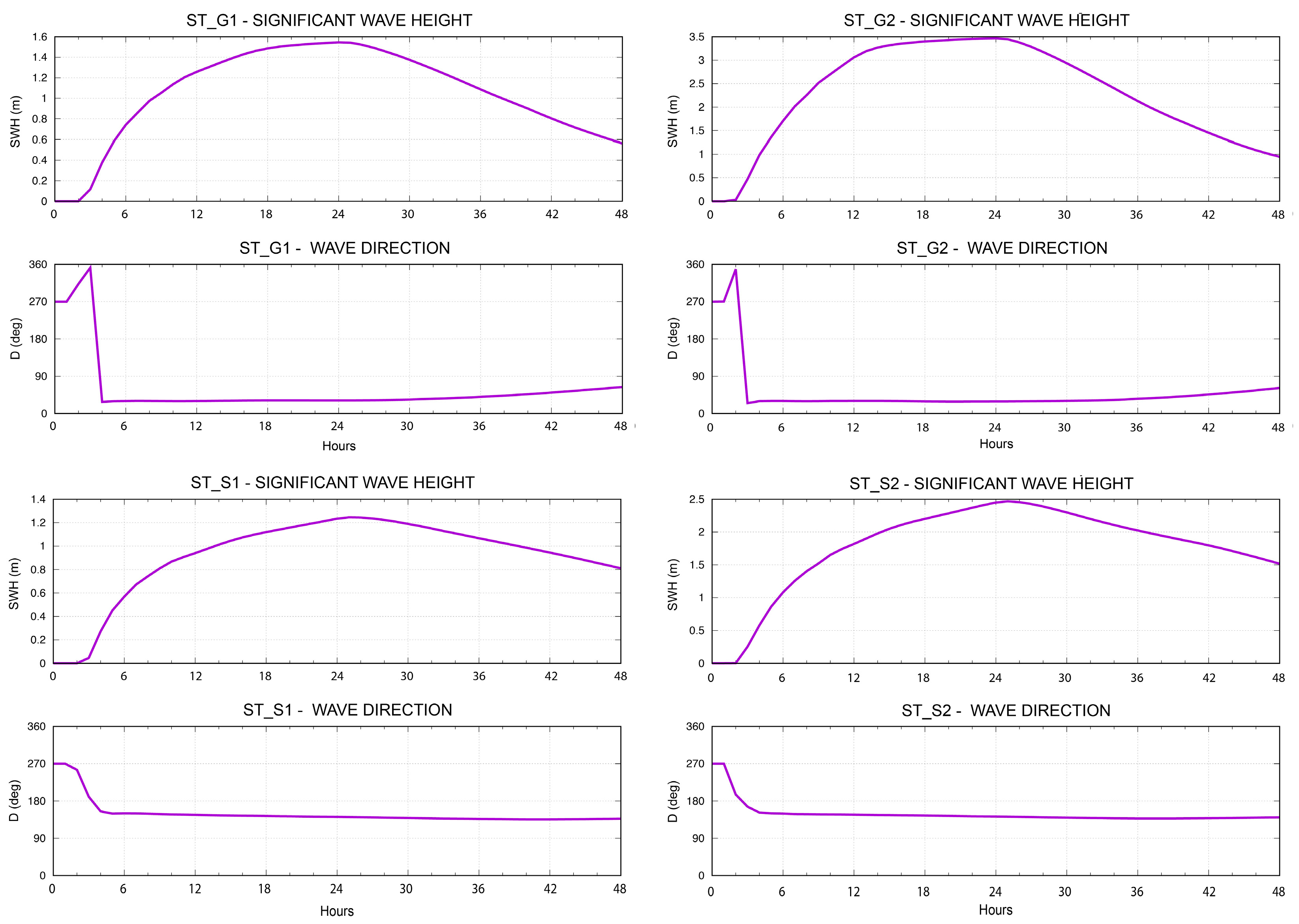In Figure 5 the SWH distribution was reported for each scenario as reproduced by the model for the first 2 days of the whole simulated period at the offshore location in front of both study sites. The linear increasing in time of the wind intensity generates an asymptotic increment of the wave height up to the end of the 1st day of simulation then decreasing to 0 at the end of the 3rd day of simulation. The maximum SWH values were 1.55 m (ST_G1) and 3.51 m (ST_G2) for the Grecale scenarios and 1.21 m (ST_S1) and 2.48 m (ST_S2) for Sirocco scenarios with, constant directions of 37° and 155° for Grecale and Sirocco cases, respectively.

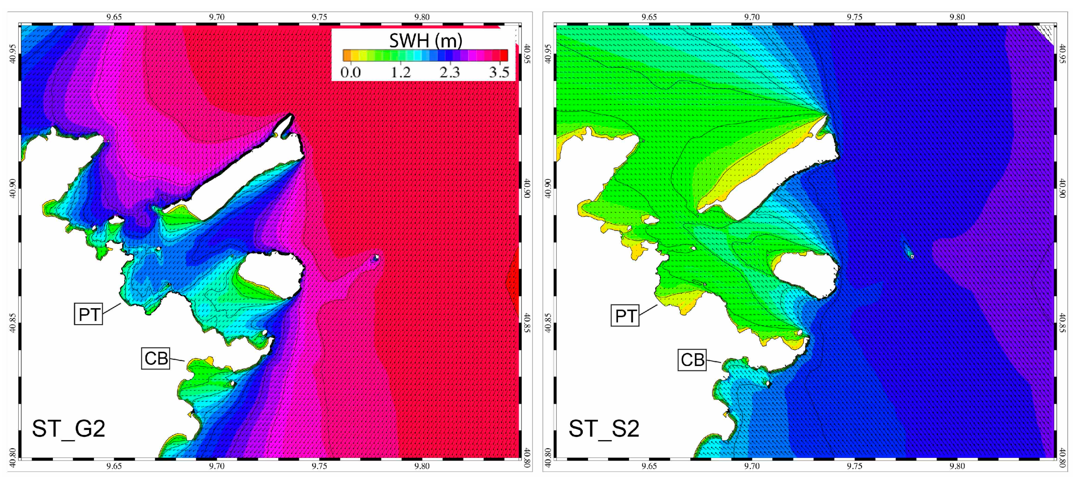
In Figure 6 the wave fields computed for the ST_G2 and ST_S2 scenarios are reported for the extended part of the domain at the end of the 1st day of the simulation, corresponding to the most energetic moments. The results highlight that the morphology of the coastal area, with the presence of capes and islands, promoted the partial sheltering of the two study sites from the direct impact of the wave fields, with the PT site sheltered from the Sirocco incident waves and the CB from the Grecale waves regime, respectively. Consequently, for the PT site, only the Grecale events, as the one reproduced by the ST_G2 in Figure 6, generated wave trains approaching directly to the shore whereas, for the CB site, only the Sirocco events, as the one reproduced by the ST_S2 in Figure 6, produce incident waves propagating directly to the shore without being deflected or blocked by the geometrical features of the coast.

As a consequence, for the PT site, the SWH in the proximity of the shore was generally higher than 1 m for both the Grecale scenarios, whereas, only in the case of a strong Sirocco event (ST_S2), the SWH inside the PT bay was appreciable with values around 0.5 m. On the contrary, for the CB site, the SWH in the proximity of the bay was always lower than 1 m in both the Grecale scenarios, with higher values obtained from scenario ST_S2, whereas for Sirocco scenarios the SWH was generally higher than 1 m in proximity of the coast.

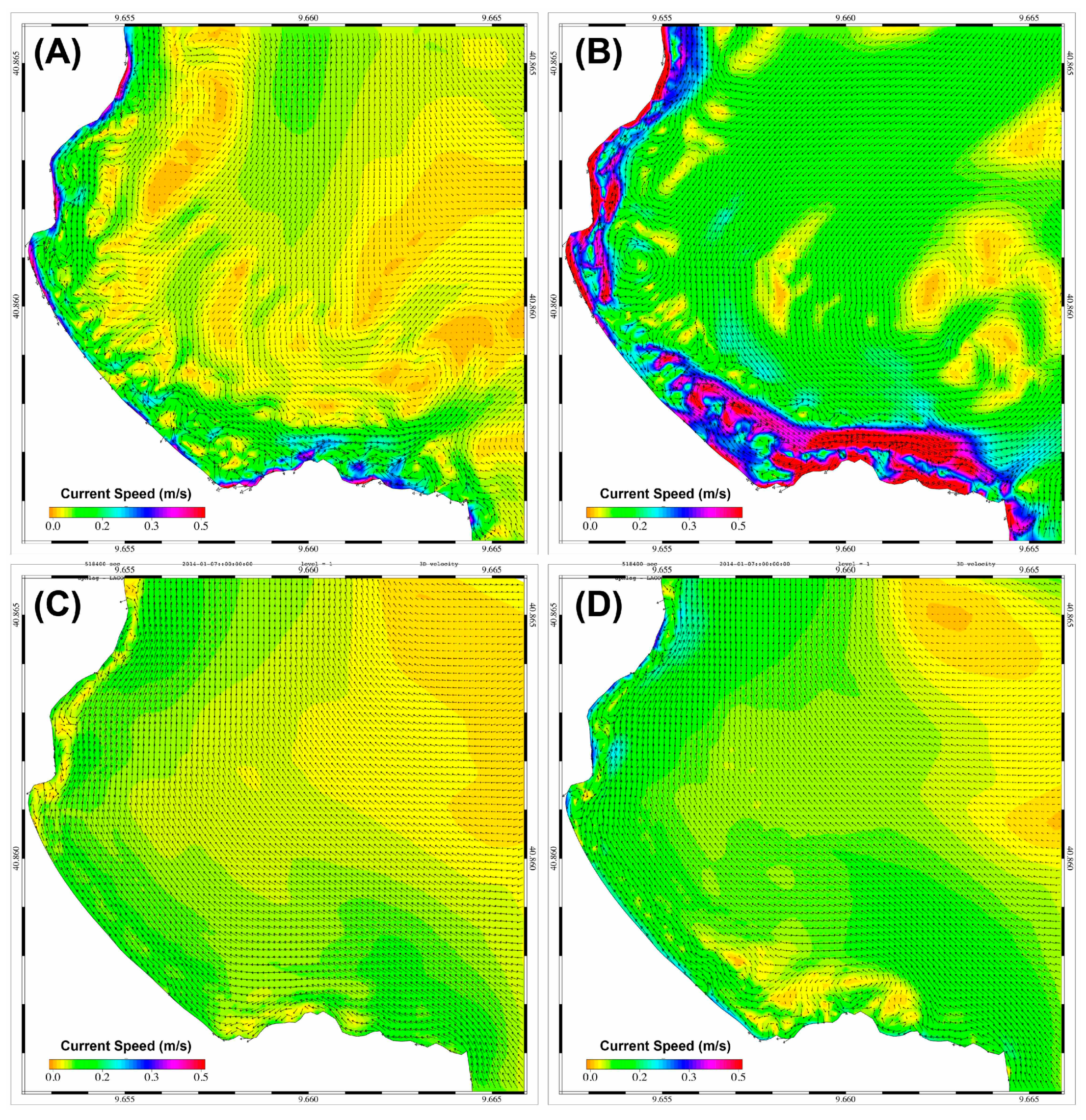
In Figure 7 the vertically averaged water circulation induced by the wave and the wind in the PT bay, as obtained at the end of the 1st day of the simulation, was reported for all the simulated scenarios. In the ST_G1 (see Figure 7, panel A) the water current field was characterized by an external flow generally directed onshore characterized by speeds around 0.1 m/s. In the proximity of the shore, the flow splits into a northward branch lapping the coast with speeds up to 0.3 m/s and a southward branch characterized by similar intensity but generating a clockwise gyre in proximity of the northern limit of the beach. A similar current pattern was obtained for the ST_G2 scenario (see Figure 7, panel B) with a northward near-shore flow and a southern clockwise gyre. In this scenario, due to the highest wind and wave intensity, the current speed was higher with values of about 0.5 m/s obtained in the proximity of the shore in the northern part of the beach. For both scenarios the effects of the wave action on the littoral flow were evidenced by the presence of several recirculation cells overlapping the general circulation pattern.

The results obtained by the Sirocco scenarios, ST_S1 and ST_S2, evidenced that, due to the lower wave energy impacting on the shore, the water circulation was mainly modulated by the direct action of the wind. In fact, the vertically averaged current patterns, depicted in panels C and D of Figure 6, were mainly homogeneous and directed to the northwest along the whole shore, therefore following the direction of the wind forcing. The wave-induced circulation cells were found only in the ST_S2 scenario and in correspondence of the northern and southern limits of the beach where, due to refraction and diffraction processes, the direct impact of waves partially occurred.

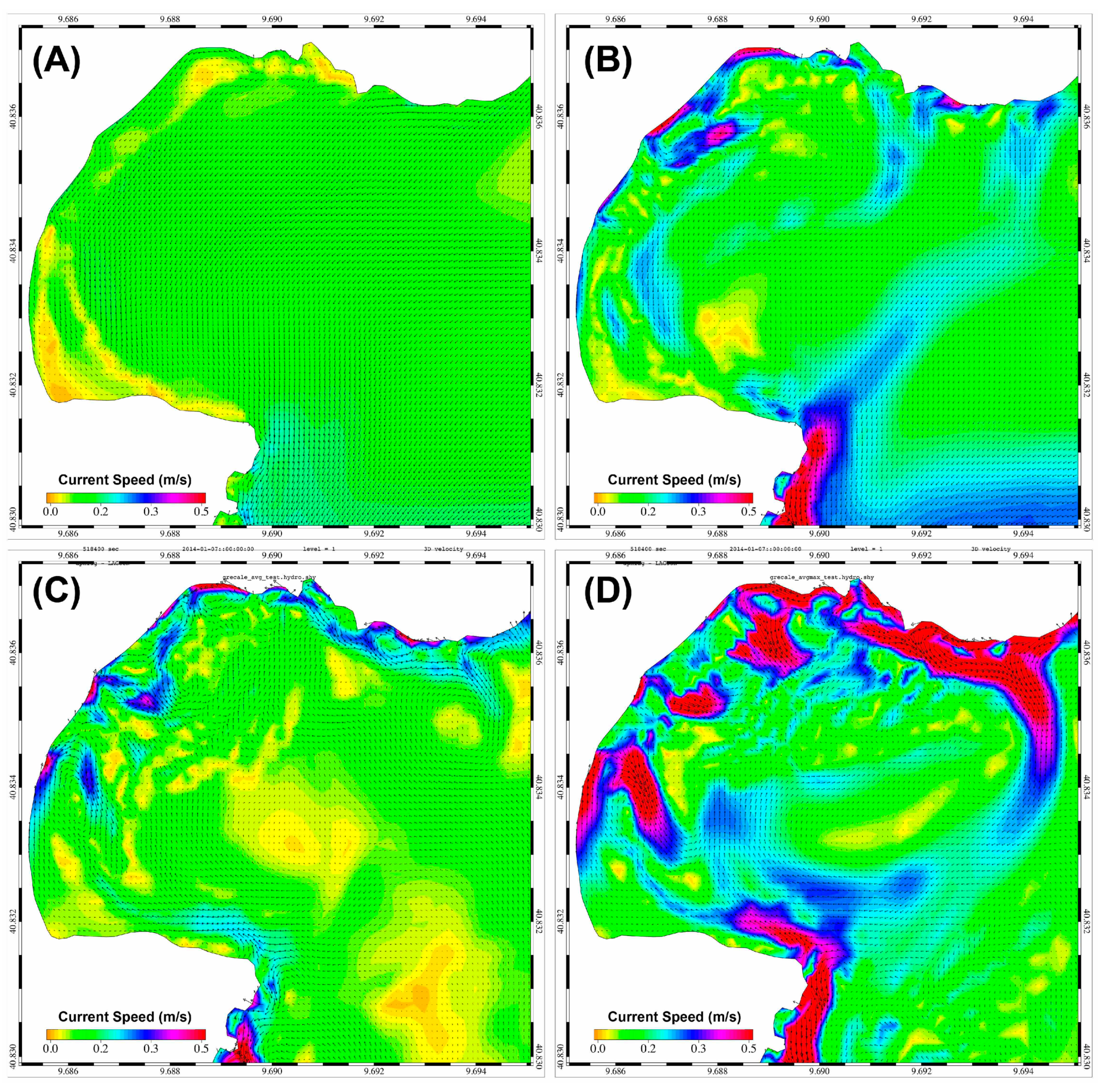
In Figure 8, the results obtained by the four different scenarios were reported for the CB bay at the moment the SWH was maxima. In this case, the Grecale wave action was generally not influencing the littoral water circulation. In fact, in the ST_G1 (see Figure 8, panel A), the water circulation was mainly directed southward as a direct consequence of the wind action. Only in the southernmost tip of the beach, the wave forcing contributed to the generation of anticlockwise circulation cells overlapping the general circulation. The current speed was generally low with values around 0.2 m/s.

In the ST_G2 (see Figure 8, panel B) the increasing of the wave energy impacting the shore due to the refraction and diffraction processes generated an increment of the current speed intensities up to 0.3 m/s. The wind action induces a general southward alongshore flow, but, in this scenario, the higher wave energy impacting onshore promotes the growth of two macro recirculation cells splitting the bay into a northern clockwise area and a southern anticlockwise area converging in the middle in correspondence of an offshore flow (rip current).

In the case when the Sirocco blows and the induced waves impact directly on the shore, as the scenarios ST_S1 and ST_S2, the vertically averaged water circulation was generally stronger, with values higher than 0.5 m/s (see panel C and D of Figure 8). For both scenarios, the external part of the bay was characterized by the presence of a macro anticlockwise circulation cell, which dragged the coastal waters from the northern part of the bay to the South. In the proximity of the shore, the combined action of the wind and waves promotes the generation of several circulation cells and local intense offshore flows in correspondence of the convergence zones between the cells.

3.3. PO Leaves Transport

The transport of the PO leaves due to the waves and currents starts when the wave runup reaches the banquettes on the shoreline and immersion processes take place. Specifically, the transport of the numerical particles, continually released on the shore boundary elements, was simulated when the distance (DM) from the shoreline reached by the incident wave was higher than 2 m, a threshold established on the basis of the PO dumping practice (see Section 2.2.2). 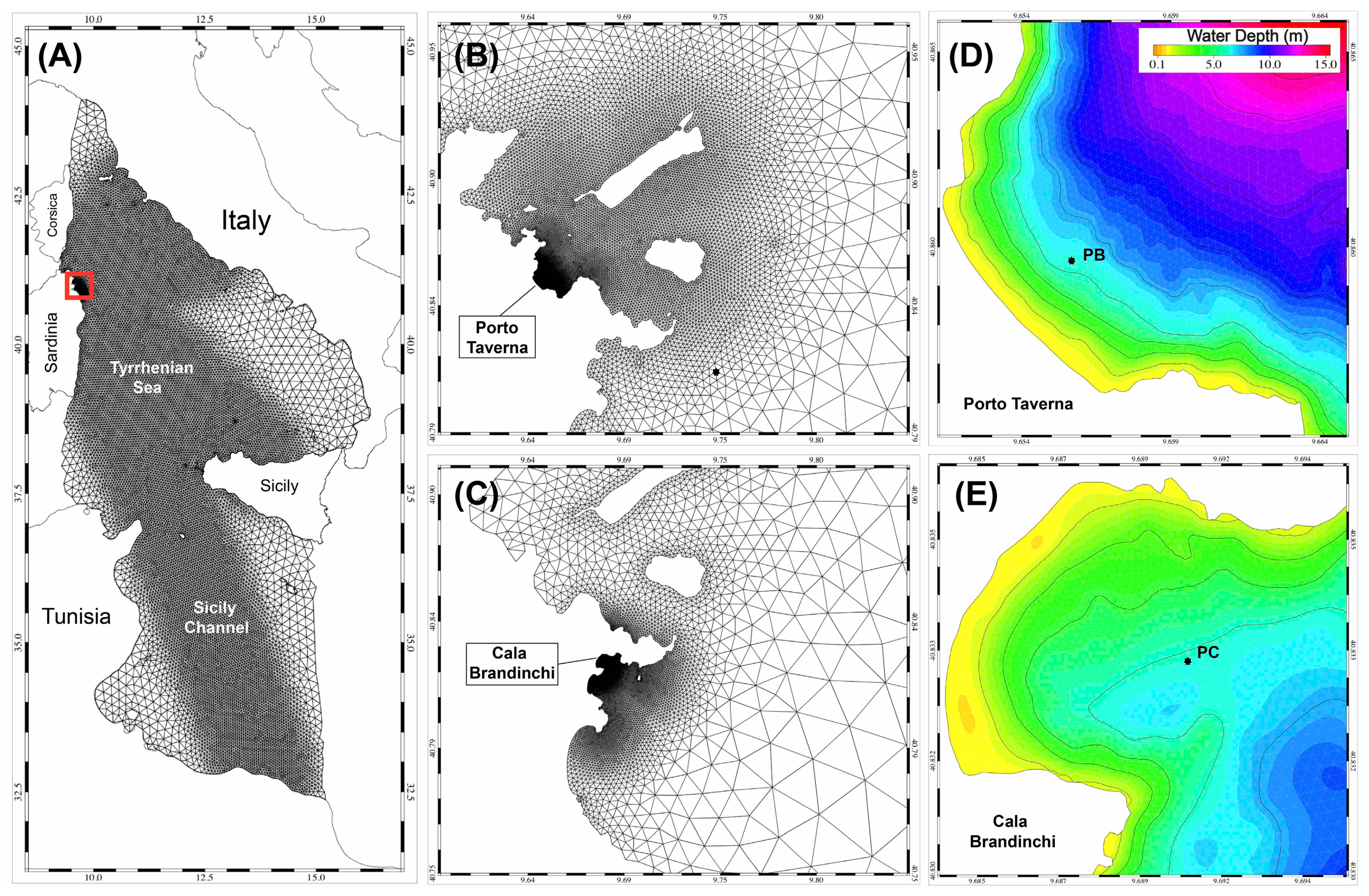According to Equation (1) (see Section 2.2.2), the DM values were computed for all the scenarios and for both the study sites, considering, as input data, the time series of T and SWH obtained from the simulation results for positions located in front of the two beaches offshore of the breaking line at around 5 m water depth (see PB and PC in Figure 4).

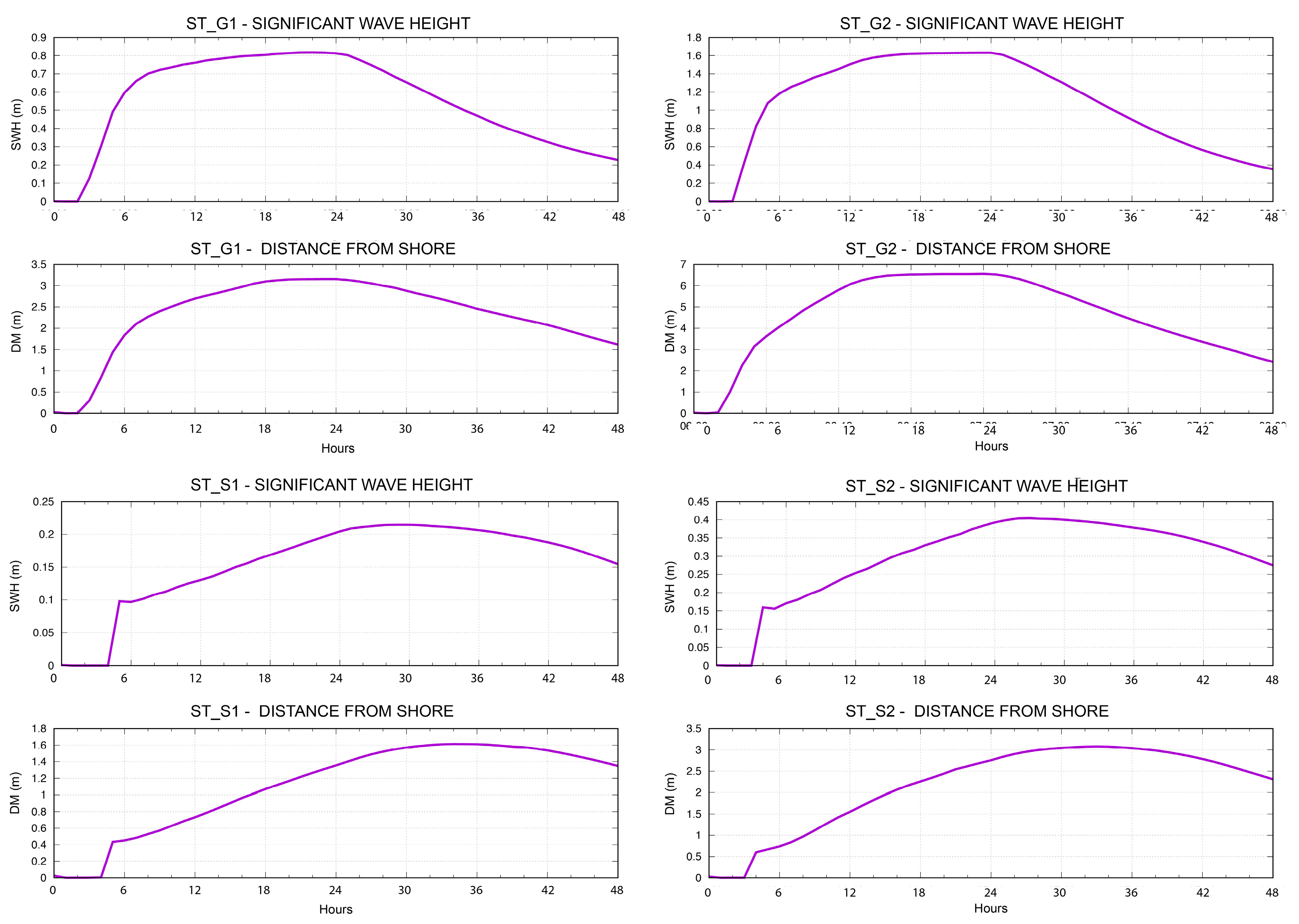
In Figure 9, the time evolution of the DM values along with the SWH computed at the reference location for the PT study site was reported for the whole set of simulated scenarios. For the Grecale scenarios, the SWH in front of the beach reached maximum values between 0.8 and 1.6 m, determining maximum DM values varying between around 3, in the ST_G1, and 6 m, in the ST_G2. Considering the 2 m DM threshold for the banquette immersion, the transport of the leaves started 6 h later than the beginning of the storm event, in the ST_G1 scenario and, just 3 h later in the ST_G2 case. Assuming the leaves immersion occurring only for the growing phase of the storm event (see Section 2.2.2), the release of the numerical particles from the PT shore was simulated for about 18 h in the ST_G1, and for about 21 h in the ST_G2. Once immerged, all the processes affecting the fate of the PO leaves into the water, were reproduced until the end of the 3 days of the simulated period.

For the Sirocco scenarios, due to the sheltering effect of the bay geometry, the wave runup on shore was less intense, with maximum SWH varying between 0.2 and 0.4 m, generating DM values between 1.6, in the ST_S1, and 3 m in the ST_S2. As a consequence, considering the DM threshold of 2 m, only in the ST_S2, the immersion of the PO leaves was activated and, therefore, the transport processes simulated. Specifically, in the ST_S2, the immersion started about 15 h later than the beginning of the simulation and lasted for about 12 h until the maximum wave height was reached. On the contrary, being the DM threshold not overcome during the whole model run, the ST_S1 scenario was not considered for the simulation of the PO leaves transport at sea.

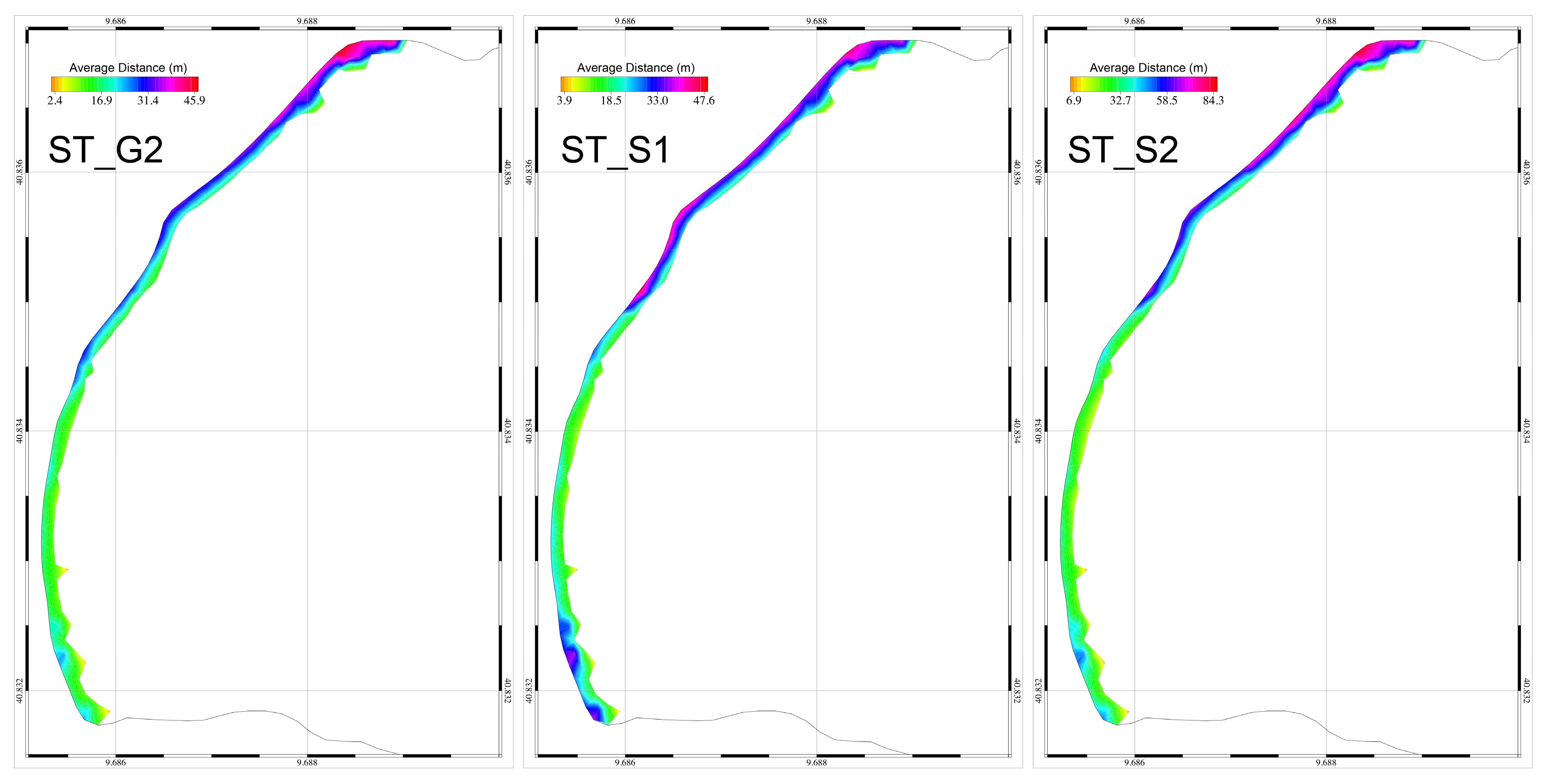
For all the scenarios in which the immersion of the numerical particles was promoted by the overcome of the DM threshold, all the in-water processes were simulated. From the simulation results, the distances from the shore of the particles deposited on the sea-bed were then computed and averaged in time for the whole simulated period.

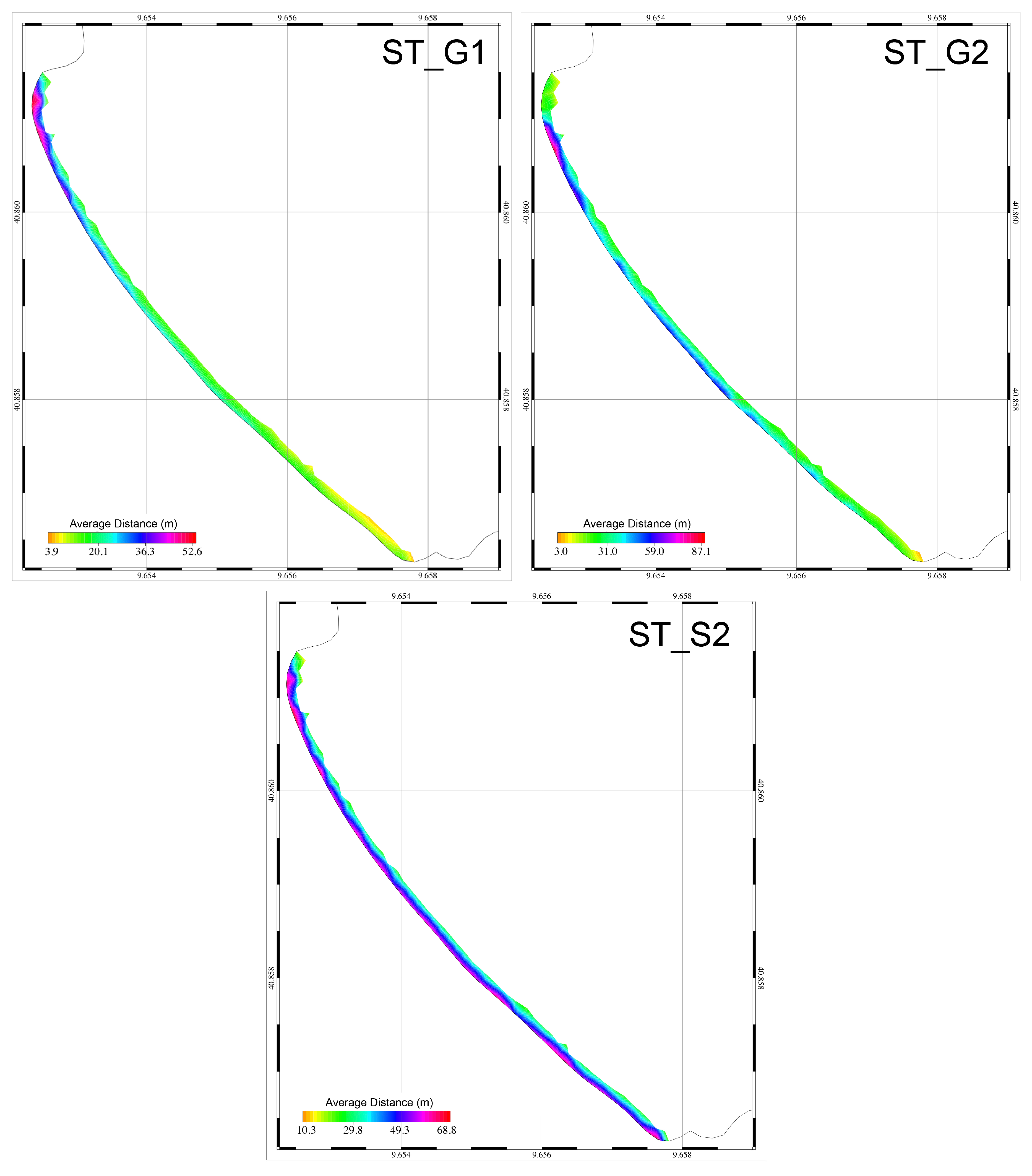
In Figure 10, the average distances from the shore reached by the released particles were reported for the PT study site, as being computed from the results of both the Grecale scenarios and of the ST_S2 scenario only. The adopted unit scales were not uniform among the scenarios results, being the scope of the analysis to investigate the relative distribution of the average distances along the shoreline. The distances from the shore varied between a few meters up to maximum values around 90 m in correspondence of the northernmost limit of the beach. The distributions obtained for the Grecale scenarios were characterized by similar patterns with a marked north to south negative gradient, with the highest distances found in the correspondence of the northern beach limit and the lowest at the southern extreme. The absolute values differ between the two scenarios due to the differences in the wind and wave intensities, with maximum distances of about 53 m in the ST_G1 and of about 88 m in the ST_G2, respectively. In the Sirocco scenario, ST_S2, the distribution was more homogeneous, with most of the values varying between 50 and 60 m and with the highest values, around 69 m, localized in the northern beach sector.

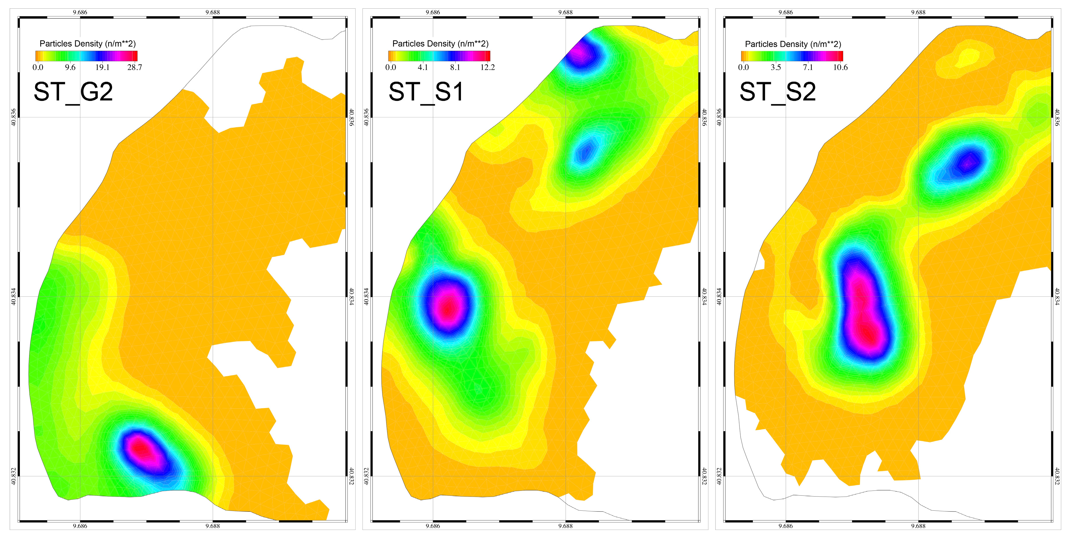
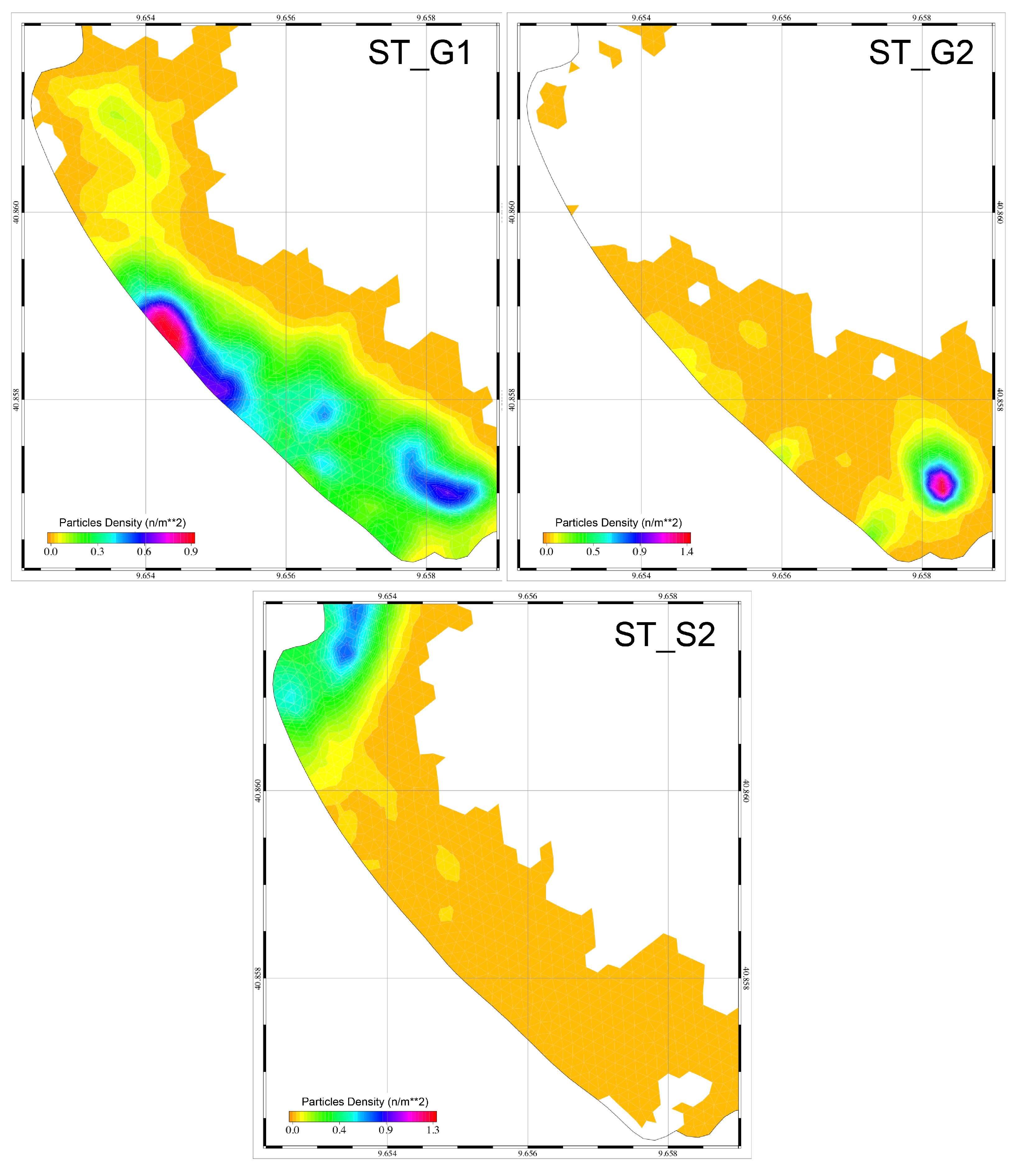
The deposition of the PO leaves simulated by the numerical particles is one of the main processes determining the patterns described in Figure 10. In Figure 11 the spatial distribution of the averaged particle density that is deposited at the seabed was reported for the two Grecale scenarios and for the ST_S2. Similar to the previous case, the unit scales were not uniform among the scenarios results, being the scope to highlight the relative distribution of the deposition patterns in the bay. Similar patterns were found for the two Grecale scenarios with two relative peaks localized near-shore in the middle of the bay and in front of the northern beach limit. The differences between densities values were mainly related to the transport efficiency of the current in the two cases. In fact, the higher particle densities in the ST_G1 were promoted by a lower capacity of the flow field to drive the particles out of the bay with the consequent increase of the local sedimentation. On the contrary, even if the circulation pattern was similar (see Figure 7 panels A and B), in the ST_G2, the higher current speeds promoted the transport of the particles out of the bay with a consequent lower local deposition. In the Sirocco case, the pattern was different indicating net south to north transport of the numerical particles, mainly generated by the wind-induced flow (see Figure 7, panels C and D), which promotes the deposition outside of the bay.

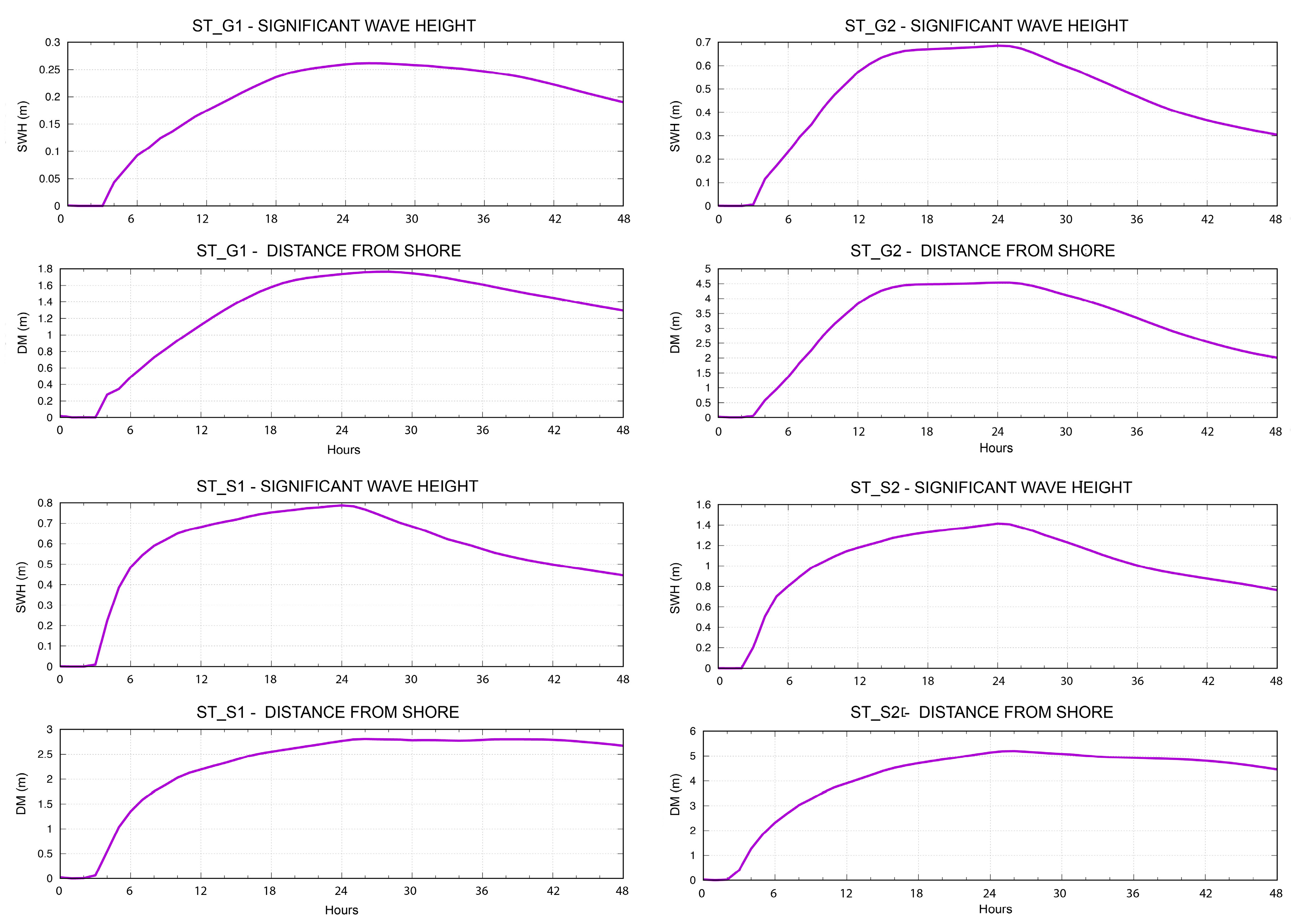
In Figure 12, the time evolution of the DM and SWH computed at the reference location for the CB study site was reported. Contrarily to the PT case, for the Grecale scenarios, only in the ST_G2, the computed SWH was capable to generate runup with DM values greater than 2 m and therefore to activate the immersion and transport of the PO leaves. For this scenario, in fact, the immersion started around 8 h later than the beginning of the storm event, when the 2 m DM threshold was overcome and lasted for about 16 h until the maximum SWH, around 0.7 m, was reached. As for PT study case, once immerged, all the processes affecting the fate of the PO leaves into the water were reproduced until the end of the 3 days of the simulated period. On the other hand, in the less energetic scenario, ST_G1, the SWH was always lower than 0.3 m with maximum DM around 1.8, a value lower than the threshold for activating the immersion and the transport of the PO leaves. Consequently, for this scenario the in-water transport processes were not simulated.

For the Sirocco scenarios, the maximum SWH values varied between 0.8 and 1.4 m, generating maximum DM values varying between 2.8 and 5.1 m, in the ST_G1 and ST_S2, respectively. For both cases, the 2 m DM threshold for the banquette immersion was overcome and the leaves transport simulated starting 10 h later the beginning of the storm event, in the ST_G1 scenario, and 5 h later in the ST_G2 case. The numerical particles were continuously released from the CB shore for about 14 h in the 1st Sirocco scenario, and for about 19 h in the second one.

For the ST_G2 and for both the Sirocco scenarios, all the in-water processes were simulated and, the average distances from the shore of the particles deposited on the seabed, computed. In Figure 13, the average distances from the shore were reported for the CB study site, as being computed from the results of the ST_G2 scenario and of both the Sirocco scenarios. Unit scales were not uniform among the scenarios results, being this analysis focused to highlight the relative differences in the average distances distribution along the shore. Similar to the previous case, the distances from the shore varied between a few meters up to maximum values around 90 m. For all the scenarios the distributions were characterized by similar patterns with a marked north to south negative gradient, with highest distances found in correspondence of the northern beach limit and lowest in the middle with a slightly increase in the southern extreme. The absolute values differ between the scenarios due to the differences in the wind and wave intensities and directions, with the maximum distances from the shore varying between 40 and 50 m for the ST_G2 and ST_S1, and 85 m for the ST_S2.

In Figure 14 the spatial distribution of the average particle density at the seabed was reported for the ST_G2 and for the two Sirocco scenarios. Similar to previous cases, and for the same motivations, unit scales were not uniform among the scenarios results. The differences in the density values were mainly related to the transport efficiency of the currents in the different cases. In the Grecale scenarios, the deposition pattern was characterized by a peak localized in the southernmost part of the bay in front of the cape limiting the CB beach. This distribution was mainly ruled by the wind-induced circulation, which promoted a north to south flow within the bay (see Figure 8, panels A and B). On the contrary, in both the Sirocco scenarios, the water circulation was mainly modulated by the wave action (see Figure 8, panels C and D) and the obtained deposition pattern was characterized by the presence of two relative maxima located in the northern and southern part of the bay, respectively. In these scenarios, the particles sedimentation was modulated by the rip currents between the circulation cells, which dragged the particles offshore until the flow intensity was higher than the sedimentation threshold, below which the deposition occurred.

4. Discussion

The results obtained by the set of simulations describing different meteo-marine scenarios were processed in order to provide practical information for managing the practice of dumping the PO leaves on the shoreline of the two studied sites.

For both beaches, only three meteo-marine scenarios activated the immersion of the PO leaves and the subsequent simulated transport and deposition processes. The obtained results evidenced that the patterns describing the average distances from the shore reached by the particles when deposited were similar when considering scenarios characterized by the same meteo-marine regime (see Figure 10 and Figure 13). In fact, for these cases, the main differences between the distributions obtained by the low and the high scenarios were on the absolute reached distances and in the activation or not of the immersion processes. On the other hand, comparing the results obtained by scenarios describing different meteo-marine regimes, the obtained results differ not only in the absolute values of the average distances but also in the relative distribution pattern.

As a consequence, averaging and normalization procedures were applied to obtain a consistent and easy to use indication on the best positions along the shoreline where releasing the PO leaves. In particular, for each case study, the average distance distributions obtained from each meteo-marine scenario (see Figure 10 and Figure 13) were normalized in relation to the relative maximum obtained value. For each element of the domain representing the shoreline, a weighted averaging procedure of the three normalized values obtained by the three simulated scenarios was then applied. The weights were calculated from the statistics of the wave climate reported in the polar plot of Figure 3, identifying, first of all, the SWH intervals, higher than 1 m, characterizing each forcing scenario obtaining for ST_G1 characterized by with SWH=1.5 m (see Table 2), the values between 1 and 2 m, for ST_G2, with SWH=3.5 m (see Table 2), the values between 2 and 3 m, for ST_S1, with SWH=1.2 m (see Table 2), the values between 1 and 2 m, and finally for ST_S2, with SWH=2.5 m (see Table 2), the values between 2 and 3 m. For these SWH intervals and for the Grecale and Sirocco directions, the relative number of occurrences during the winter–autumn period were obtained from data depicted in the polar plot of Figure 2 (panel b), corresponding to the 10%, 4%, 11%, and 3% of the total events. Therefore, assuming the Grecale and Sirocco regimes accounting for the 100% of the useful events for the immersion and transport of the PO leaves, and considering, for each case study, only the three scenarios producing the RDI results, the relative percentage of occurrence was calculated. As an example, for the PT case, being the ST_G1, ST_G2, and the ST_S2 the only scenarios allowing the PO leaves immersion, and being their occurrences during the winter–autumn seasons equal to 10%, 4%, and 3%, their relative percentages of occurrence corresponded to 58%, 24%, and 18% for the ST_G1, ST_G2, and ST_S2, respectively. Consequently, the adopted weights in the averaging procedure corresponded to 0.58 for the ST_G1, 0.24 for the ST_G2, and 0.18 for the ST_S2, in the PT case, whereas to 0.61 for the ST_S1, 0.17 for the ST_S2, and 0.22 for the T_G2, in the CB case.

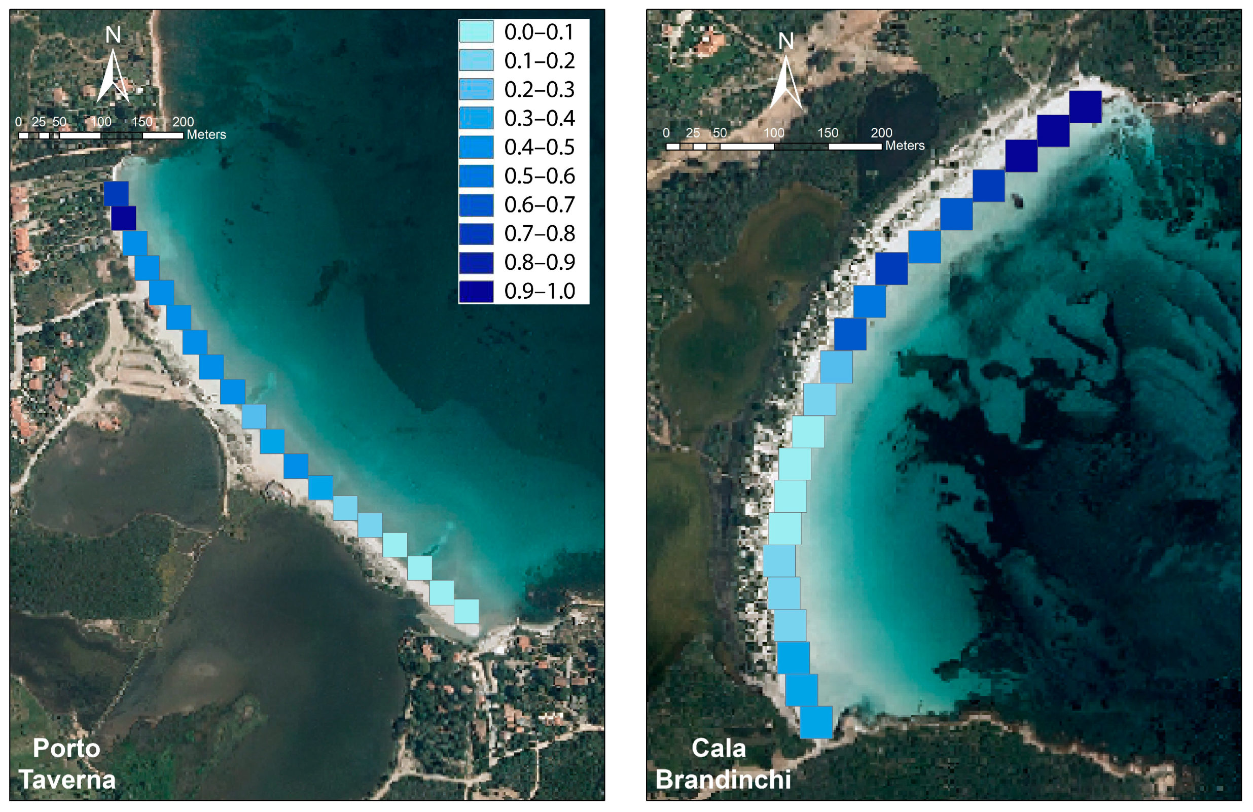
From the weighting averaging procedure, the relative dispersion index (RDI) was computed for each boundary element of the two domains constituting the beaches shorelines. The computed values were then processed to obtain a regular spatial distribution of the RDI on a set of 25 m length squares centred on the beach shoreline. In Figure 15 the a-dimensional relative dispersion index, RDI, was reported for the PT and CB case studies. The results highlight that, for the PT beach, the northern sector of the shoreline was the most suitable for dumping the PO leaves being this part of the beach more efficient for transporting the particles far from the coastline. On the other hand, the RDI distribution obtained for the CB beach indicates that both the central and northern parts of the shoreline were ideal positions for releasing the PO leaves with the guarantee of an efficient transport far from the shoreline.

This analysis was not considering either the absolute distances reached by the particles in relation to the different meteo-marine forcing, nor the transport efficiency characterizing each scenario. The followed procedure, in fact, was suited to indicate the best location for the release of the PO leaves, a practice that is carried out independently from incoming storm events or predicted meteorological conditions. Therefore, the choice of the locations where to release the PO leaves should account only for the local average meteo-marine conditions without evaluating the efficiency of the transport induced by specific storm events.

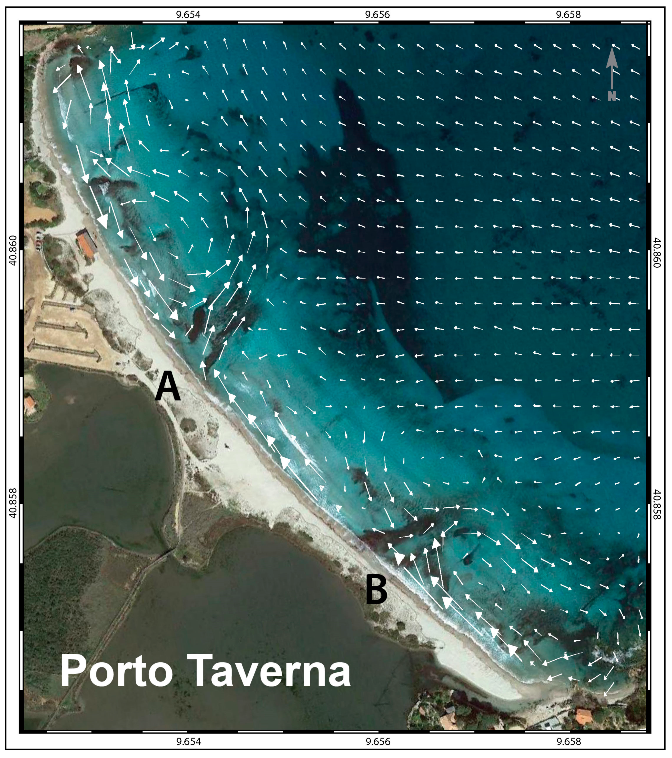
The absence of wave and current data collected in the near-shore area makes it impossible to carry out a quantitative validation of the model results in reproducing the wave and current dynamic in the two study cases. However, considering the purpose of this application aimed to provide indications on the relative variability of the PO leaves dispersion efficiency along the coastlines, the model results were qualitatively compared with satellite imagery (Google Earth, see https://www.google.com/earth/ for further iformation) [36] of the PT beach area at the time a moderate wind storm hit the coast. The comparison shows a correct reproduction of the coastal circulation patterns evidenced by a clear matching between the currents vector fields produced by the model and the patterns of the PO debris at the sea bottom, which are shaped by the near-shore circulation induced by the wind and wave action. The analysis and the obtained results are detailed in Appendix B. The adopted approach, even if based on a qualitative analysis, indicates that the model application was capable of reproducing the main features of the flow field, which is the main factor determining the variability of the dispersion coefficient, the RDI, along the coastline. In future works aimed to provide further management indications for the PO leaves disposal as, not only the best positioning along the coast, but also the most efficient meteo-marine event promoting the dispersion of the PO leaves at sea then wave and current measurements should be collected in the near-shore area to perform a quantitative assessment of the model accuracy.

Another aspect to be considered in future works is the amount of sediments trapped and adhered to the PO leaves that could vary along the coastline due to the wave and currents impacts on the sediment deposition processes. As a consequence, the sinking velocity of the leaves could be not uniform, affecting, therefore, the PO leaves surface transport and bottom deposition. These processes should be taken into account particularly in the cases of beaches with grain sizes varying between fine and very fine sand and with a high component of carbonatic grains.

Furthermore, in this modelling study any information about the size of the seagrass beach-cast deposits was not considered. For roughly a decade, both study sites were certainly subjected to the practice of the banquettes removing, thus, the quantification of the seagrass annual deposits and of their distribution along the shore was not feasible. Nevertheless, the adopted averaging and normalization procedure allowed us to compute the relative distribution of the dispersion efficiency of the different locations where the PO leaves can be released, which is independent of the released quantities and therefore can be adopted as helpful criteria for the selection of the dumping sites.

The proposed approach to the management of the beach-cast seagrass wracks is therefore useful to guarantee both the tourist usability of the beaches during the summer months and to avoid the increasing costs of storage and removal of the PO leaves, which, if released in areas not favouring the immersion and transport far from the shoreline, could accumulate year after year. Furthermore, the particles deposition patterns obtained from numerical simulations, indicate that the PO leaves, once immerged and wetted, in most of the scenarios, are deposited at the seabed in front of the shore and, generally, within the bay, guaranteeing a net nutrient flux, which is essential to restore the energy balance altered by the banquettes removal during the spring months.

At the present, the management of banquettes on the beaches of PT and CB follow the directives issued by the regional authority, which do not contain any indications on the areas where the banquettes should to be repositioned along the shore. The proposed approach indicates the locations where a more efficient dispersion of the banquettes should to be expected, reducing, therefore, the long-term management costs for those Institutions, as the MPAs, that have in charge the seasonal removal and repositioning practices.

Up to now, in fact, any scientific study or investigation on the dispersion at the sea of the material repositioned on beach faces was not available for managers to select the suitable areas for the repositioning practice. In this study, for the first time, we investigated the fate at sea of the PO leaves repositioned along the beach faces, providing practical indications on the most suitable areas where releasing the deposits. This approach is important from a management standpoint providing a robust and scientific based alternative to the random and subjective choice of the areas where banquettes should be repositioned.

5. Conclusions

The P. oceanica banquettes are currently managed along several areas of the Mediterranean with different practices varying between the temporary removal and repositioning during autumn and winter, the permanent removal and the no removal. Although most of the national authorities promote the third option, often the local managers prefer to remove the banquettes and to reposition them on the shore during autumn and winter. The choice of the dumping location can have a great impact on the permanence of the banquettes on the beach. In fact, observation on beaches along the Mediterranean Sea highlighted that a huge amount of banquettes can resist several months in the beach face, therefore increasing their management costs during the summer season and generating conflict with the recreational usage of the littorals.

For these reasons the present study represents a pilot experiment that provided scientific basis and technical support to local managers that chose the temporary removal and repositioning of the P. oceanica banquettes along the littorals. It is also aimed to spread good practices and homogenize local, independent actions through the adoption of standardized methods that could guarantee wide applicability and environmental sustainability.

In order to determine the local oceanographic conditions and to identify the most suitable sites for autumnal repositioning of the P. oceanica leaves the authors adopted a numerical approach. Two beaches, Porto Taverna (PT) and Cala Brandinchi (CB) located along the eastern coast of Sardinia Island, an area characterized by both the presence of P. oceanica meadows and for the intense recreational usages of the littorals, were considered as study sites.

Specifically, for both sites, the wind waves and water currents dynamics representative of the prevalent meteo-marine conditions of the area were reproduced by applying a high resolution hydrodynamic and wave model. Successively, for each meteo-marine scenario, the transport of the seagrass wracks at sea was investigated using a particle tracking model reproducing the main physical processes affecting the fate of the P. oceanica leaves dispersed at sea.

The obtained results were analysed and a relative dispersion index (RDI) for the seagrass deposits released along the two shores was calculated. The RDI allowed identifying those sectors of the shoreline most suitable for the dumping of the P. oceanica wracks in relation to the efficiency of the leaves transport far from the coastline.

Specifically, for the two study cases, PT and CB, this application identified several areas, mainly located in the northern sectors of the tow beaches, characterized by a higher RDI indicating an ideal positioning for releasing the P. oceanica leaves during the autumn and winter periods.

The obtained results indicate the proposed approach to the management of the beach-cast seagrass wracks as a useful tool to avoid the increasing costs of the yearly storage and removal of the P. oceanica leaves which, if released in areas not favouring an efficient transport far from the shoreline, could accumulate year after year. The proposed approach, in fact, provided a detailed framework of the residence times of the banquettes on the beaches, which can help managers in the selection of the site where a banquette should be repositioned.

Furthermore, the localization of the areas suitable for the repositioning of the leaves would allow a natural redistribution of the biomass and sediments by the waves and currents. In this way, the material is reinserted into the natural cycle of the coastal system. Furthermore, the application of this technique would avoid the costs associated with the cleaning of the leaves to retain the sediment in the beach and would avoid the costs associated with the disposal of the leaves.

During the last decade several EU funded projects such as STRATUS (see http://interreg-maritime.eu/web/stratus/progetto for further information), POSBEMED (see https://posbemed.interreg-med.eu/el/ for further information), and BARGAIN (see https://www.isprambiente.gov.it/en/projects/inland-waters-and-marine-waters/bargain for further information) focused on the development and application of management models of the different drivers and pressures acting on the beach environment including those aspects related to the removal of the seagrass wracks from the shorelines. The followed method based on specific oceanographic model applications provided important indications useful for the management of this type of practice and can be extended to all different types of beaches along the Mediterranean coasts.