Article

Numerical Simulation of Large Wave Heights from Super Typhoon Nepartak (2016) in the Eastern Waters of Taiwan

1
Department of Hydraulic and Ocean Engineering, National Cheng Kung University, Tainan City 70101, Taiwan
2
National Science and Technology Center for Disaster Reduction, New Taipei City 23143, Taiwan
3
Department of Geosciences, National Taiwan University, Taipei City 10617, Taiwan
*
Author to whom correspondence should be addressed.
J. Mar. Sci. Eng. 2020, 8(3), 217; https://0-doi-org.brum.beds.ac.uk/10.3390/jmse8030217
Submission received: 2 March 2020 / Revised: 16 March 2020 / Accepted: 17 March 2020 / Published: 20 March 2020
(This article belongs to the Special Issue Storm Tide and Wave Simulations and Assessment)

Abstract

:
Super Typhoon Nepartak (2016) was used for this case study because it is the most intense typhoon that made landfall in Taiwan in the past decade. Winds extracted from the Climate Forecast System version 2 (CFSV2) and ERA5 datasets and merged with a parametric typhoon model using two hybrid techniques served as the meteorological conditions for driving a coupled wave-circulation model. The computed significant wave heights were compared with the observations recorded at three wave buoys in the eastern waters of Taiwan. Model performance in terms of significant wave height was also investigated by employing the CFSV2 winds under varying spatial and temporal resolutions. The results of the numerical experiments reveal that the simulated storm wave heights tended to decrease significantly due to the lower spatial resolution of the hourly winds from the CFSV2 dataset; however, the variations in the storm wave height simulations were less sensitive to the temporal resolution of the wind field. Introducing the combination of the CFSV2 and the parametric typhoon winds greatly improved the storm wave simulations, and similar phenomena can be found in the exploitation of the ERA5 dataset blended into the parametric wind field. The overall performance of the hybrid winds derived from ERA5 was better than that from the CFSV2, especially in the outer region of Super Typhoon Nepartak (2016).

Graphical Abstract

1. Introduction

Typhoons are usually associated with extreme wind waves and storm surges, impacting navigational safety, infrastructure in nearshore and offshore waters (harbors, seawalls, lighthouses, etc.), and coastal habitats [1,2,3,4,5]. The oceanic and coastal hazards caused by typhoon-driven storm waves pose a greater threat to human life, property, and infrastructure than storm surges in Taiwan. This is particularly true when a super typhoon makes landfall in Taiwan. A typhoon is designated as a “super typhoon” when its wind speeds near the typhoon center exceed 114 kt (equivalent to 58 m/s) and its intensity reaches category 4 or 5 on the Saffir–Simpson scale [6]. A super typhoon ranks among the most destructive natural hazards worldwide because it produces high storm surges, large storm waves, and torrential downpours [7]. For instance, a seawall at a fishing port near the southeastern coastal waters of Taiwan was broken in 2018 by large storm waves from several typhoons (as shown in the upper-right panel of Figure 1); a lighthouse located in a fishing port in the southeastern offshore waters was destroyed by Super Typhoon Meranti-induced extreme storm waves in 2016 (as shown in the lower-right panel of Figure 1). Therefore, accurately predicting, simulating and hindcasting typhoon-induced storm wave heights is important for the prevention and mitigation of disasters in the ocean and along coasts [2,3,4]. Assessments of typhoon-generated extreme wave heights with different return periods are very useful for designing seawalls to protect boats, ships, nuclear power plants, and coastal critical infrastructures from wave impacts. Moreover, the strength evaluation of oil platforms and wind turbine supporting systems is highly dependent on simulating extreme waves accurately [8,9].
A comprehensive understanding of the ocean surface waves arising from extreme weather conditions is of great interest to coastal and ocean engineers and oceanographers. Many studies about predicting, simulating, or hindcasting typhoon-generated storm waves and storm surges have been carried out through numerical models because wave buoys cannot be deployed throughout an entire marine area [10,11,12,13,14]. A third-generation spectral wind wave model is mainly driven by wind fields and has been widely used to predict, simulate, and hindcast wave heights. Therefore, accurate wind forcing data are essential for predicting sea states with great accuracy, especially with extreme waves created by typhoons [4]. Moreover, improvements in wind forcing for wave-circulation models are believed to enhance the performances of large wave and large surge simulations [4,5,15].
The objective of the present study is to assess the effects of wind sources from different spatial and temporal resolutions on storm wave height simulation and to investigate the optimal hybrid typhoon winds through two approaches for the best performance of storm wave height simulation during Super Typhoon Nepartak in 2016. The paper is organized as follows: Section 2 describes the typhoon, observational data, bathymetry, wind forcing, and coupled wave-circulation model that were used in the present study. Section 3 presents the comparisons between the simulations and measurements for the significant wave height (SWH) time series using different wind fields. Section 4 provides a discussion of the results from a series of numerical experiments. Finally, a summary and conclusions are presented in Section 5.

2. Data and Methodology

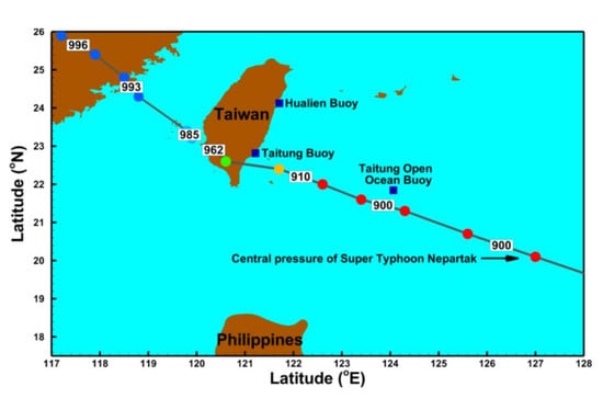
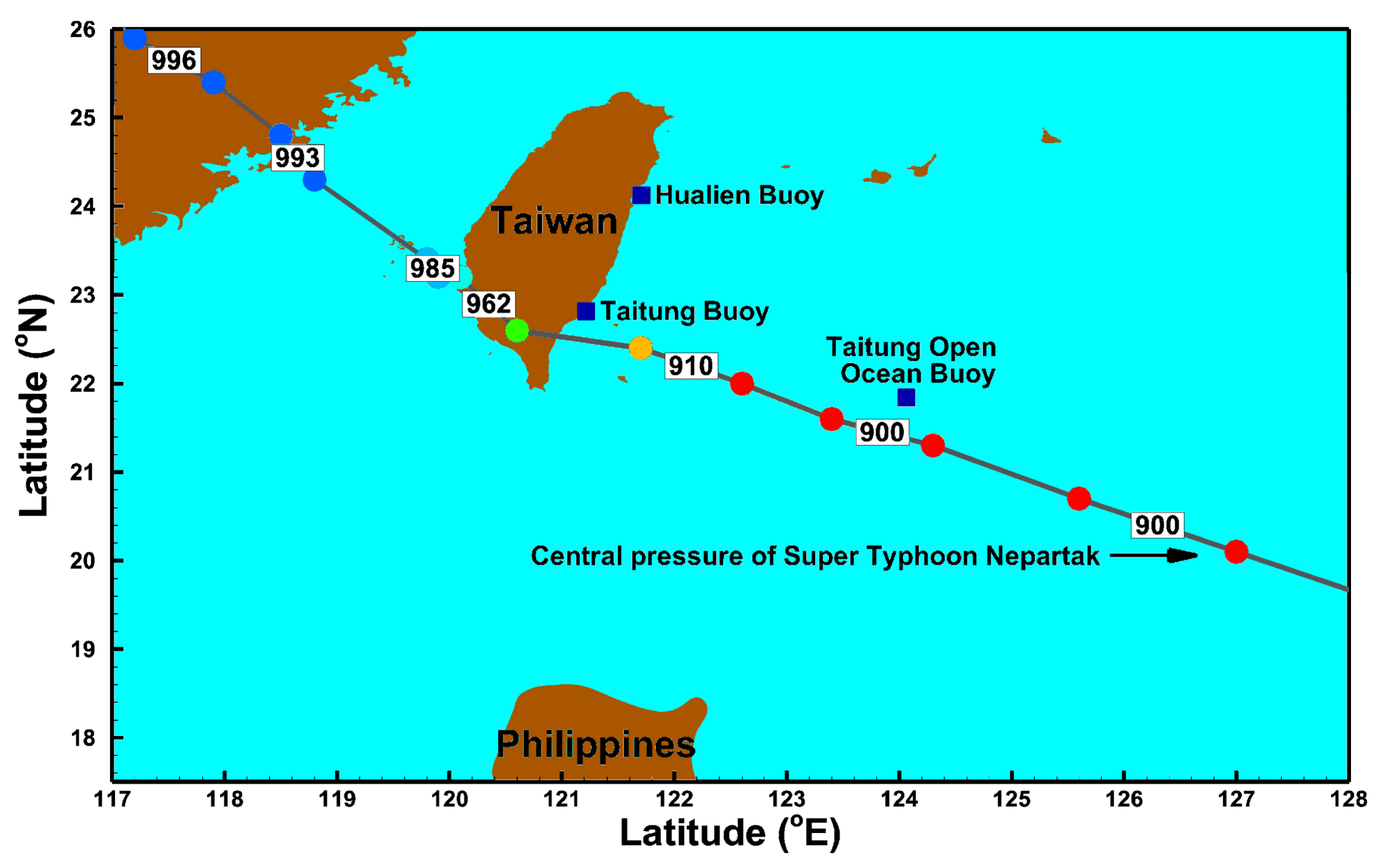
2.1. Super Typhoon Nepartak (2016)
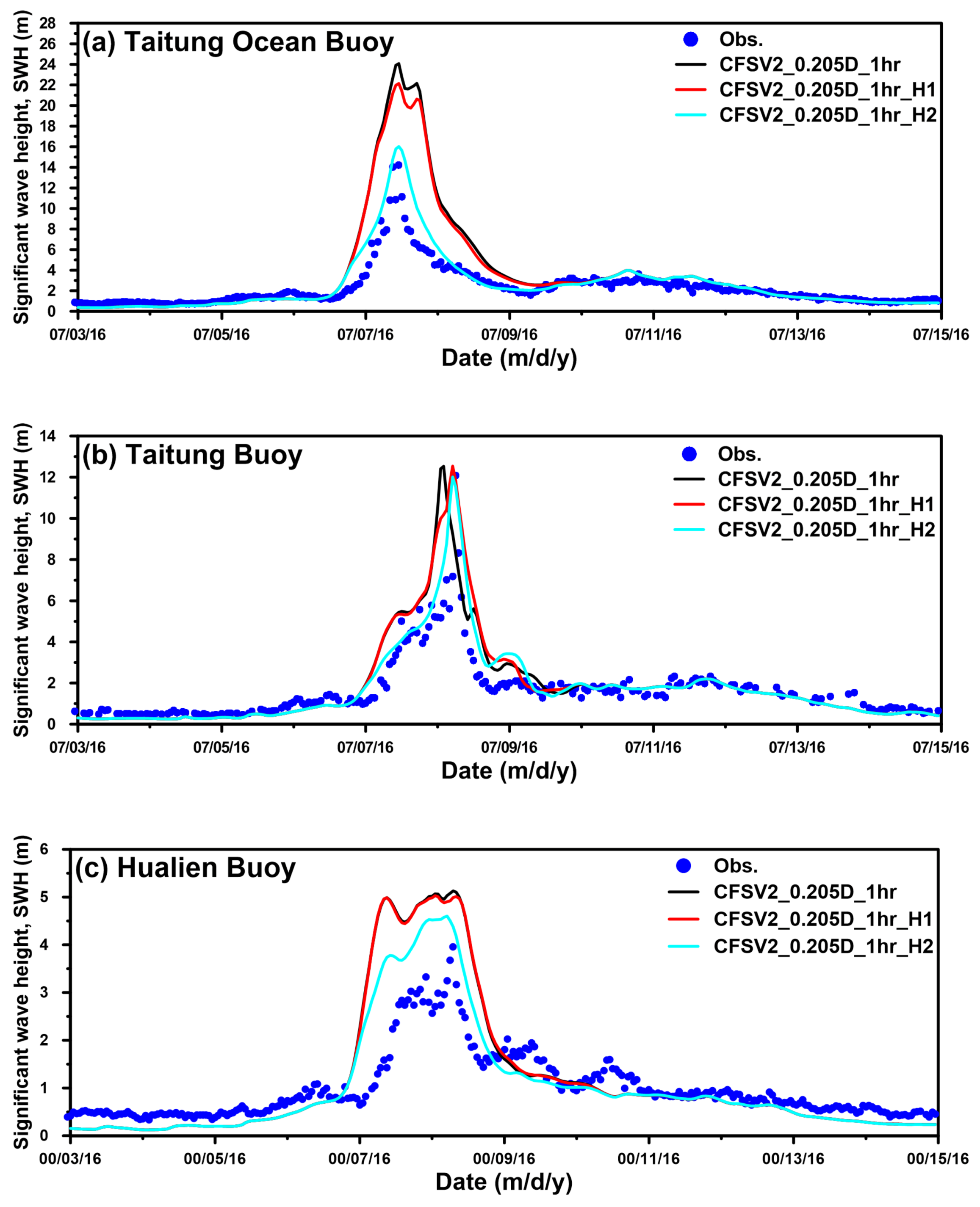
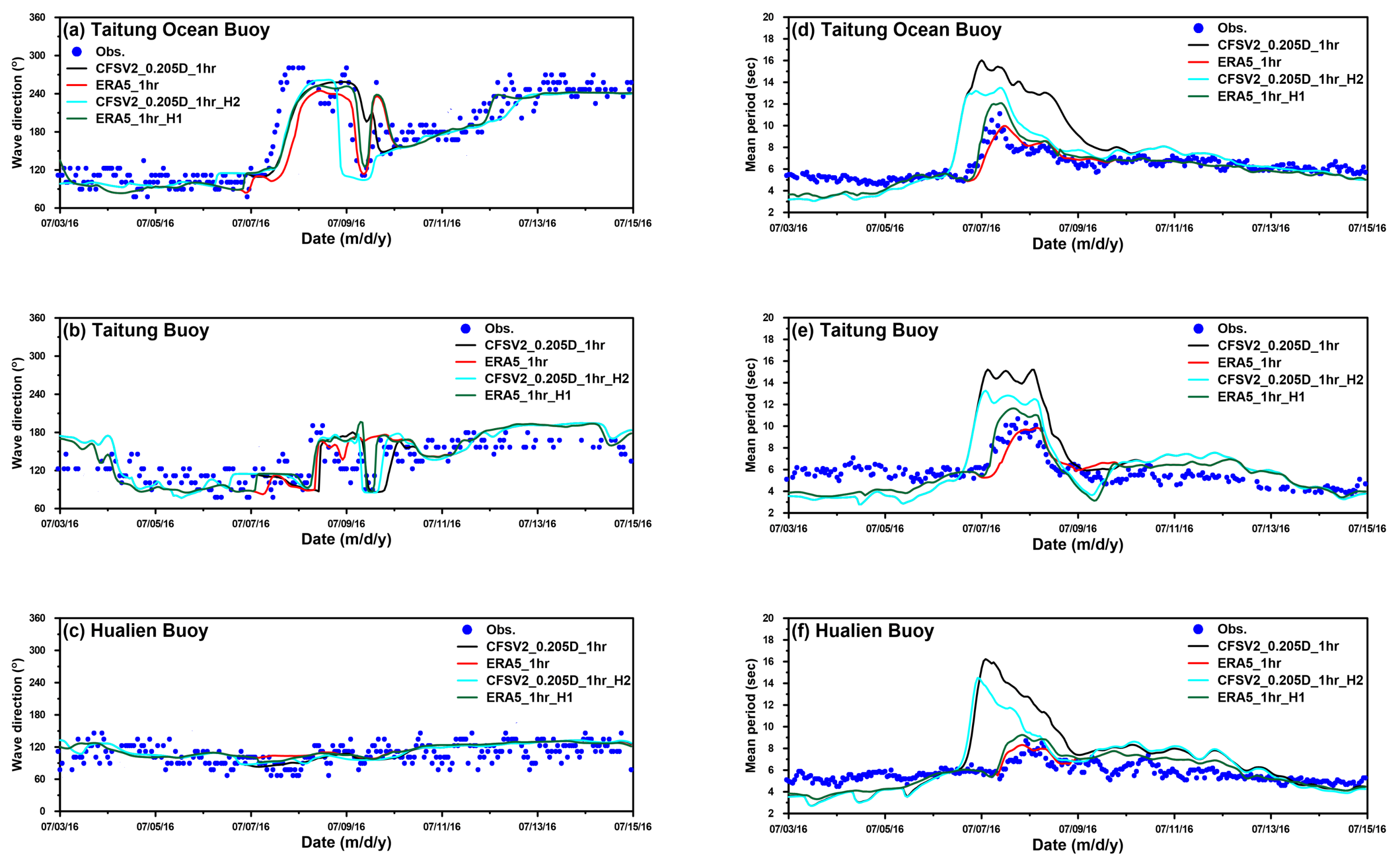
Super Typhoon Nepartak was the third most intense tropical cyclone worldwide in 2016. It initialized in the southern waters of Guam on 30 June and was subsequently named Nepartak by the Japan Meteorological Agency (JMA) after it had intensified into a tropical cyclone on 3 July. The Joint Typhoon Warning Center (JTWC) of the United States upgraded Nepartak to a category 4-equivalent super typhoon on 5 July and estimated that Nepartak had become a category 5-equivalent super typhoon the next day. Super Typhoon Nepartak reached its peak intensity approximately 835 km east-southeast of Taitung County, Taiwan, on 6 July; meanwhile, the JMA evaluated 10-min maximum sustained winds of 205 km/h and a central pressure of 900 hPa. Super Typhoon Nepartak made landfall in Taitung County and subsequently moved into the Taiwan Strait from Tainan County on 8 July. After that, Typhoon Nepartak continued moving inland into China as a tropical depression and dissipated on 10 July. According to the report from the Central Weather Burau (CWB) of Taiwan, Meranti was the most intense typhoon that had made landfall in Taiwan in the past 10 years (2010–2019). Figure 2 demonstrates the track and central pressure (intensity) of Super Typhoon Nepartak (2016).

2.2. Wave Buoy

The hourly SWH measurements recorded at three wave buoys by the CWB, Taiwan, in the eastern waters of Taiwan during Super Typhoon Nepartak (2016) were acquired to evaluate the optimal wind field for simulating typhoon-driven SWHs. The wave buoys record the SWH, wave direction and mean wave period, and wind speed and direction at 2 m height above sea level with a sampling frequency of 2 Hz, and an accuracy of ±10 cm for the SWH. The locations of the three wave buoys, namely, the Hualien, Taitung, and Taitung Ocean buoys, are shown in Figure 2, and their corresponding coordinates and water depths are listed in Table 1.

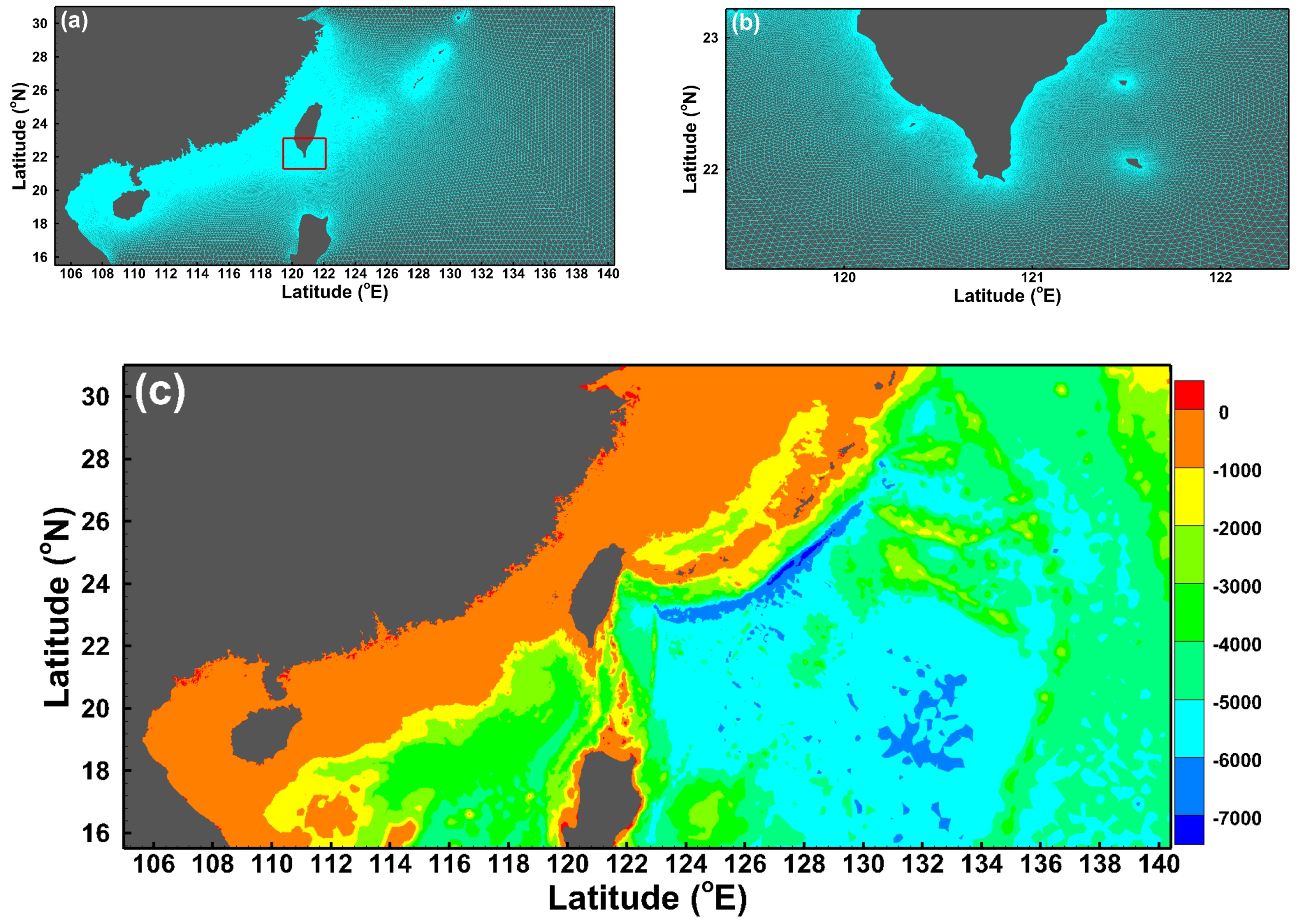
2.3. Description and Configuration of the Wave-Circulation Model

In the present study, the hydrodynamics of the waters surrounding Taiwan were simulated from 1 to 20 July 2016, by means of the semi-implicit cross-scale hydroscience integrated system model (SCHISM). The SCHISM was developed by Zhang et al. [16] with many improvements and enhancements from the original semi-implicit Eulerian–Lagrangian finite-element (SELFE) model, [17]. The SCHISM employs finite-element, finite-volume methods and hydrostatic and Boussinesq approximations to solve the shallow water equations. The SCHISM eliminates the Courant–Friedrichs–Lewy (CFL) stability restrictions due to the application of the semi-implicit schemes for all governing equations. The numerical stability constraints are further relaxed because the nonlinear advection terms in the momentum equations are treated with a Eulerian–Lagrangian method. The introduction of the no-mode-splitting technique in the SCHISM contributes to eliminating numerical errors regarding the splitting between internal and external modes [18]. SCHISM and SELFE have been widely used for simulating the inundation associated with storm surge [19,20,21], assessing the effects of sea-level rise on tidal current energy [22] and predicting flash floods in mountainous areas [23]. Typhoon-induced hydrodynamics can be well mimicked by depth integration, i.e., a 2D model; moreover, a 2D model requires fewer computing resources and less model execution time than a 3D model. Thus, a 2D model is preferred to a 3D model for storm surge, storm tide, and wind wave modeling, and the depth-integrated version of the SCHISM, SCHISM-2D, was used in the present study. A time step of 120 s and a Manning coefficient of 0.025 were set in the SCHISM-2D following [4,15], which are based on the numerical stability of the SCHISM-2D and the type of sea bottom material in Taiwanese waters.
The third-generation spectral wave model, called the wind wave model version III (WWM-III), was adopted in the present study since phase-averaged spectral wave models are capable of predicting and simulating sea state variations in the ocean [24]. Roland [25] overhauled not only the physics and numerical schemes of the WWM-II but also the computing efficiency of the model. The WWM-III solves the wave action equation on an unstructured grid by adopting the fractional step method proposed by [26]. The minimum and maximum directions for the simulation are 0° and 360°, respectively, while the number of directional bins is 36. The lowest and highest frequency limits of the discrete wave period are 0.03 and 1.0 Hz, respectively, which are partitioned into 36 frequency bins. The constant for computing waves breaking in shallow water areas is 0.78. The peak enhancement of 3.3 is according to the report from the Joint North Sea Wave Project (JONSWAP, [27]), and the bottom friction coefficient is set as 0.067 in the WWM-III. An efficient computation can be achieved through the employment of different time steps for hydrodynamic and wind wave models in a wave-circulation coupled modeling system, and therefore, a time step of 600 s was assigned to the WWM-III. This means that SCHISM-2D delivers the wind and depth-integrated velocities and water surface elevations to WWM-III; in addition, the wave radiation stresses for SCHISM-2D are used by the WWM-III at five hydrodynamic time intervals. The SCHISM-WWM-III has been successfully applied to generate potential storm wave hazards for Taiwan [2], evaluate the effect of the wind field on wind wave hindcasting [4], and quantify the nonlinear interactions of typhoon-induced storm tides. Details on the coupling procedures for the SCHISM-WWM-III can be found in [28].
The computational domain must be large enough to simulate storm waves and storm surges generated by typhoons traveling long distances from east to west of Taiwan. In the present study, coverage from 105°E to 140°E and 15°N to 31°N was created for the computational domain of the SCHISM-WWM-III. This area is composed of 276,639 unstructured grids and 540,510 triangular elements; coarse meshes with 20–40 km resolutions were arranged in the open ocean beyond the coastal region, while fine meshes with 200–400 m resolutions were distributed along the coastline of Taiwan and its offshore islands (as shown in Figure 3a). Using a higher resolution mesh is fundamental to an accurate simulation; however, the computing demand will increase as the mesh becomes finer. Additionally, the surf zones and shallow waters are well characterized with the mesh resolution developed in the present study (Figure 3b) according to the report from [29,30,31].
A global-scale and a local-scale dataset were incorporated into gridded bathymetric data for the SCHISM-WWM-III. The GEBCO-2019 grid is the latest global-scale bathymetric product, with a spatial resolution of 15 arcsecond, released by the General Bathymetric Chart of the Oceans (GEBCO) and has been developed through the Nippon Foundation-GEBCO Seabed 2030 Project. The local-scale dataset has a coverage from 100°E to 128°E and from 4°N to 29°N with a 200-m spatial resolution provided by the Department of Land Administration and the Ministry of the Interior in Taiwan. The combined two datasets were interpolated to represent the bottom elevation in the SCHISM-WWM-III (as shown in Figure 3c). The SCHISM-2D and WWM-III take advantage of sharing the same numerical mesh to enhance the computing efficiency.

2.4. Tidal and Atmospheric Forcing

2.4.1. Tidal Forcing

Eight main tidal constituents (M2, S2, N2, K2, K1, O1, P1, and Q1) were extracted from a regional inverse tidal model (China Seas and Indonesia, [32]) and served as the tidal boundary conditions in the SCHISM-WWM-III. Although the present study focused on wind wave simulation, an inverted barometer effect resulting from the variations in atmospheric pressure was also considered in the model.

2.4.2. CFSV2 Wind Field

The Climate Forecast System version 2 (CFSV2) is an upgrade of the Climate Forecast System (CFS) and was developed by the Environmental Modeling Center at the National Centers for Environmental Prediction (NCEP). The CFSV2 is a fully coupled model representing the interactions among the ocean, land, sea ice, and atmosphere with advanced physics, increased resolution, and refined initialization to improve the seasonal climate forecasts, which makes the CFSV2 superior to the CFS. Additionally, the same model was used in the CFSV2 and the NCEP CFS reanalysis (CFSR). The CFSV2 was implemented at NCEP as the real-time seasonal forecast system in March 2011 [33]; hence, NCEP started running the CFSV2 operationally to produce analyses and forecasts. The CFSV2 products are available at horizontal resolutions of 0.205°, 0.5°, 1.875°, and 2.5° with different time intervals.

2.4.3. ERA5 Reanalysis Wind Field

ERA5 is the fifth-generation, latest global climate atmospheric reanalysis from the European Centre for Medium-Range Weather Forecasts (ECMWF). ERA5 is based on a recent ECMWF model cycle that includes coupling with ocean waves and a land model and utilizes the 4D-Var atmospheric assimilation method. ERA5 is created at a considerably higher resolution than ERA-Interim, thus replacing the widely used ERA-Interim reanalysis soon. The global hourly ERA5 atmospheric parameters are available from the Climate Data Store over latitude–longitude grids with a 0.25° by 0.25° resolution and over 137 levels in the vertical direction. The hourly ERA5 provides a more detailed evolution of extreme severe weather events and daily updates within 3 months of real time. ERA5 now covers the period from 1979 to the present; however, it will be extended from 1950 to the present by the mid-2020s.

2.4.4. Parametric Typhoon Wind Field

Many analytical parametric typhoon models have been developed to construct or reconstruct the wind and air pressure fields of typhoons for simulating storm waves and surges due to their simplicity [34,35,36,37,38,39,40]. The modified Rankine vortex (MRV) typhoon wind model proposed by [37] provides a more accurate wind field [41,42], which is satisfactory for ocean wave and storm surge modeling [4,37,43,44] and was therefore employed in the present study. A shape parameter α is used in the MRV model to adjust the distribution of typhoon wind speed (W) in the radial direction,
W = { W max ( r R max ) α   for   r < R max W max ( R max r ) α   for   r R max
where Wmax is the maximum wind speed, Rmax is the radius of maximum wind speed, and α is specified as 0.5 based on the results from [4,40,42]. Atkinson and Holliday [45] suggested an empirical relationship for Wmax and the central pressure of typhoons (Pc):
W max = 3.44 ( 1010 P c ) 0.644
The radius of maximum wind speed (Rmax) can be described as a function of Wmax and the latitude of the typhoon’s center (φ):
R max = 46.4 exp ( 0.155 × W max + 0.0169 × φ )

2.4.5. Hybrid Typhoon Wind Field

Combining the reanalysis or dynamic and parametric typhoon winds is believed to generate a better wind field in both the near-field and far-field regions of typhoons for storm wave and surge modeling [1,4,5,15,46,47,48]. Hence, two methods were applied to construct the hybrid winds from the CFSV2 and MRV and from the ERA5 and MRV. Method number 1 (H1) blends CFSV2 (or ERA5) and MRV directly through the following formula [1]:
W H 1 = { W P r < 2 R max β 0.70 β 0.06 W P + ( 1 β ) 0.72 ( 1 β ) 0.28 W R 2 R max r 7 R max   W R r > 7 R max
where WH1 is the hybrid wind speed computed via Equation (4) and WP and WR are parametric typhoon and reanalysis winds, respectively. β = ( 7 r / R max ) / 5 , in which r is the radial distance from the center of the typhoon to an arbitrary point.
Method number 2 (H2) is recommended by [46] and can be expressed as follows:
R 1 = R O P γ R T
R 2 = R O P + ( 1 γ ) R T
W H 2 = { W P r < R 1 ( 1 λ ) W P + λ W R R 1 r R 2   W R r > R 2
where ROP is the optimal radius with a minimum mean difference between WP and WR; RT is the width of the transition zone and γ is the empirical coefficient. For comparison with H1, RT and γ were given as 5 Rmax and 0.0, respectively, in the present study. λ = ( r R 1 ) / ( R 2 R 1 ) . Details for the estimation of ROP are available in [46].

2.5. Model Performance Metrics

The model capacity for the simulation of the SWH time series during Super Typhoon Nepartak (2016) is quantified via three statistical indicators, i.e., the scatter index (SI), correction coefficient (CC) and HH (Hanna and Heinold [49]) indicators. Mentaschi et al. [50] suggested that the HH indicator provides more reliable and accurate statistical information for assessing the accuracy of numerical models. Thus, in addition to SI and CC, the HH indicator was adopted for evaluation of model performance. The three criteria are defined as:
S I = 1 n i = 1 n [ ( S i S ¯ ) ( O i O ¯ ) ] 2 O ¯
C C = i = 1 n ( S i S ¯ ) ( O i O ¯ ) i = 1 n ( S i S ¯ ) 2 i = 1 n ( O i O ¯ ) 2
H H = i = 1 m ( S i O ) 2 i = 1 n S i O i
where n is the total number of data points, Si is the simulation, Oi is the observation, and S ¯ and O ¯ are the mean values of the simulations and observations, respectively.

3. Results

The winds from the CFSV2 and ERA5, as well as winds from a combination of an MRV model with the CFSV2 and ERA5 through the different techniques were exerted on the SCHISM-WWM-III to simulate the SWHs during Super Typhoon Nepartak (2016). The effects of the spatial and temporal resolutions of the wind field on storm wave height simulation, and the model performance using the different hybrid wind fields were investigated by conducting several numerical experiments.

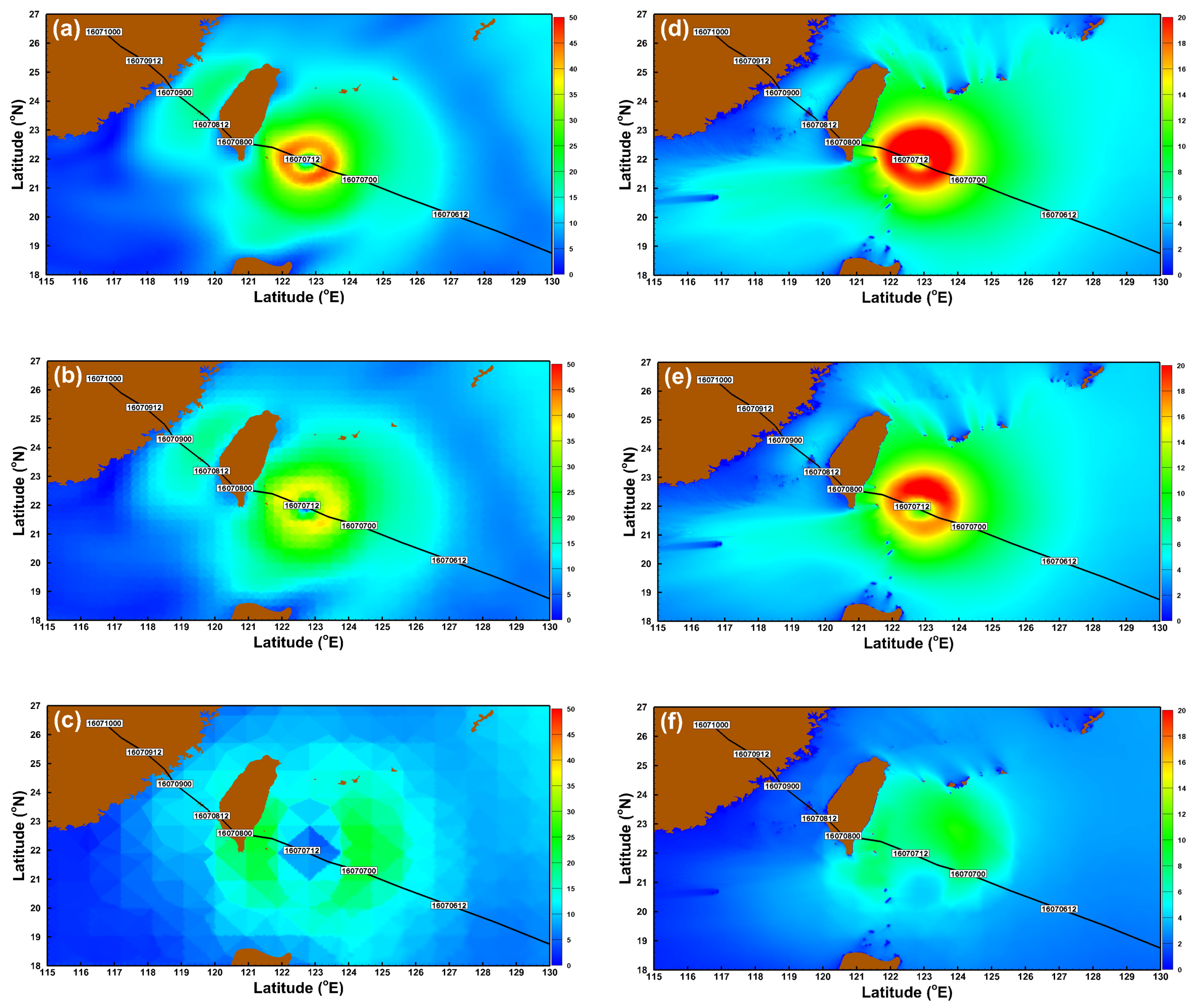
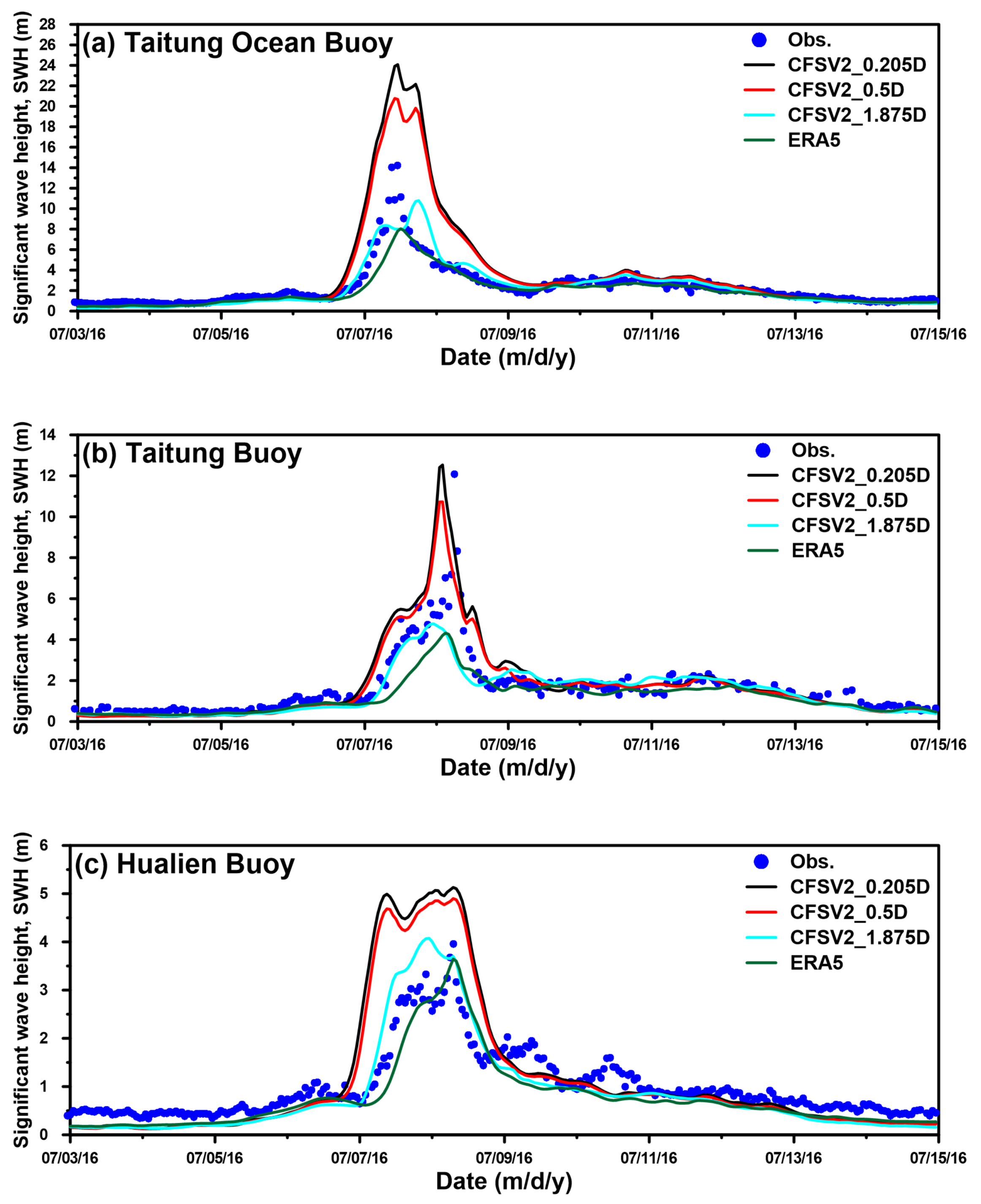
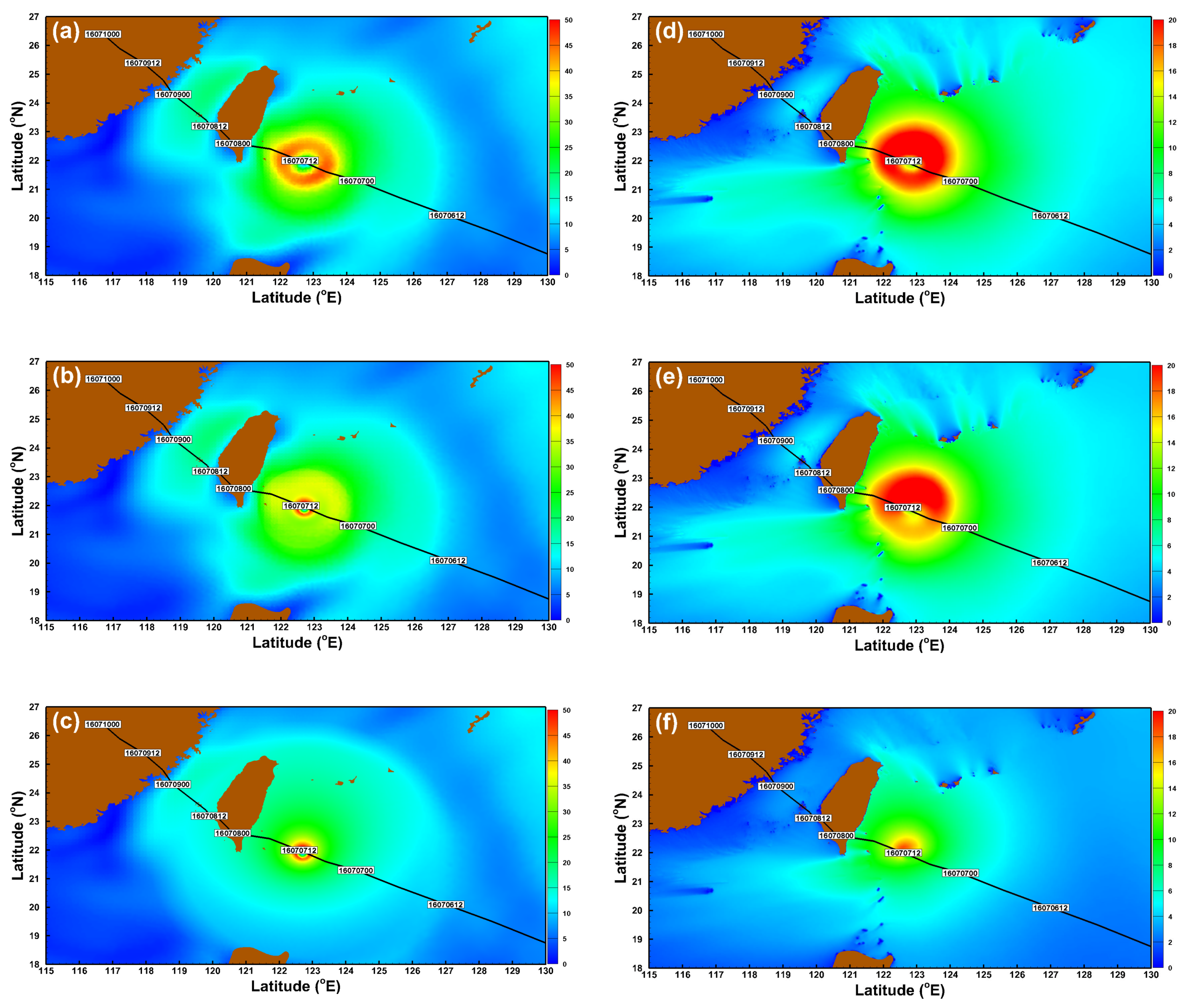
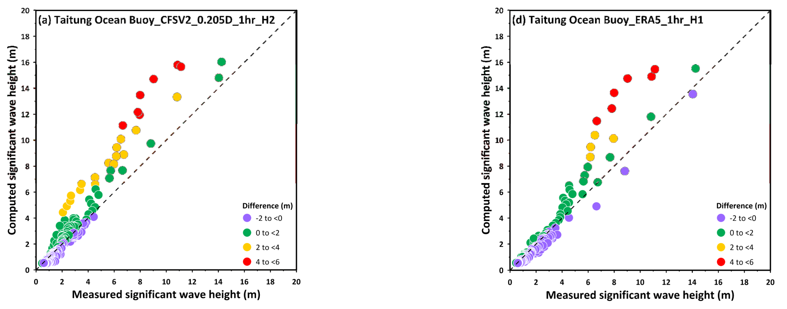
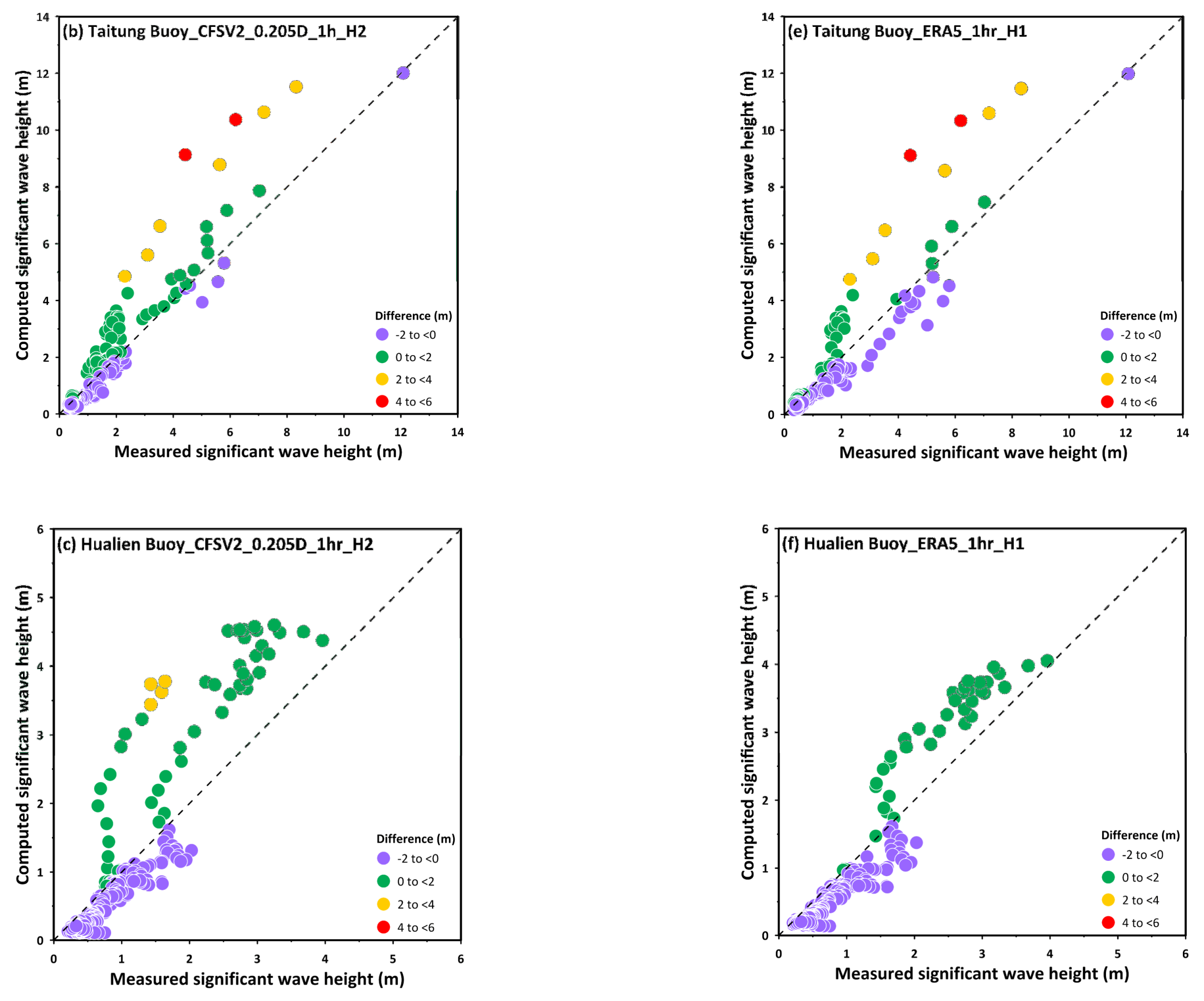
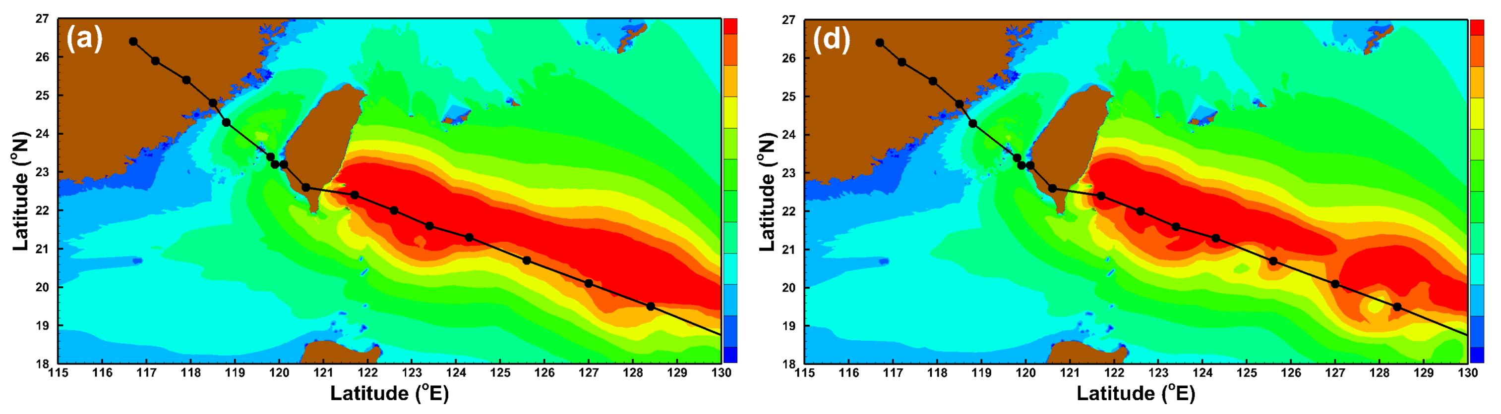
3.1. Effects of the Spatial Resolutions of Wind Fields on Storm Wave Simulation

The hourly CFSV2 winds with horizontal resolutions of 0.205°, 0.5°, and 1.875° were interpolated into the SCHISM-WWM-III. The instantaneous wind field distributions are illustrated in Figure 4a–c at resolutions of 0.205°, 0.5°, and 1.875°. Wind speeds from the hourly CFSV2 with a spatial resolution of 0.205° could reach 45–50 m/s around the near-field region of Super Typhoon Nepartak (2016) (Figure 4a); however, the wind speeds decreased dramatically when a coarser spatial resolution was used. The wind speeds of the hourly CFSV2 only reached 35–40 m/s (Figure 4b) and 20–30 m/s (Figure 4c) at 0.5° and 1.875° resolutions, respectively. Furthermore, the wind field obtained from the hourly CFSV2 with a lower spatial resolution shows a more random distribution (Figure 4b,c). The computed instantaneous SWHs corresponding to hourly CFSV2 winds with different spatial resolutions are demonstrated in Figure 4d–f. Storm waves exceeding 20 m driven by hourly CFSV2 winds at spatial resolutions of 0.205° and 0.5° could be found in the deep ocean (Figure 4d,e). Wave heights were only 8–10 m at the same time if imposing the hourly CFSV2 winds at horizontal resolution of 1.875° on the SCHISM-WWM-III (Figure 4c). Figure 5a–c shows the model-data comparisons for the SWH time series from the Taitung Ocean (Figure 5a), Taitung (Figure 5b), and Hualien (Figure 5c) buoys employing the winds from the hourly CFSV2 with different spatial resolutions. Similar to the results in Figure 4d–f, hourly CFSV2 winds at a higher spatial resolution led to the greater overestimation of storm wave heights. This phenomenon is obvious at the wave buoys near the track of Super Typhoon Nepartak (2016), i.e., the Taitung Ocean and Taitung buoys.

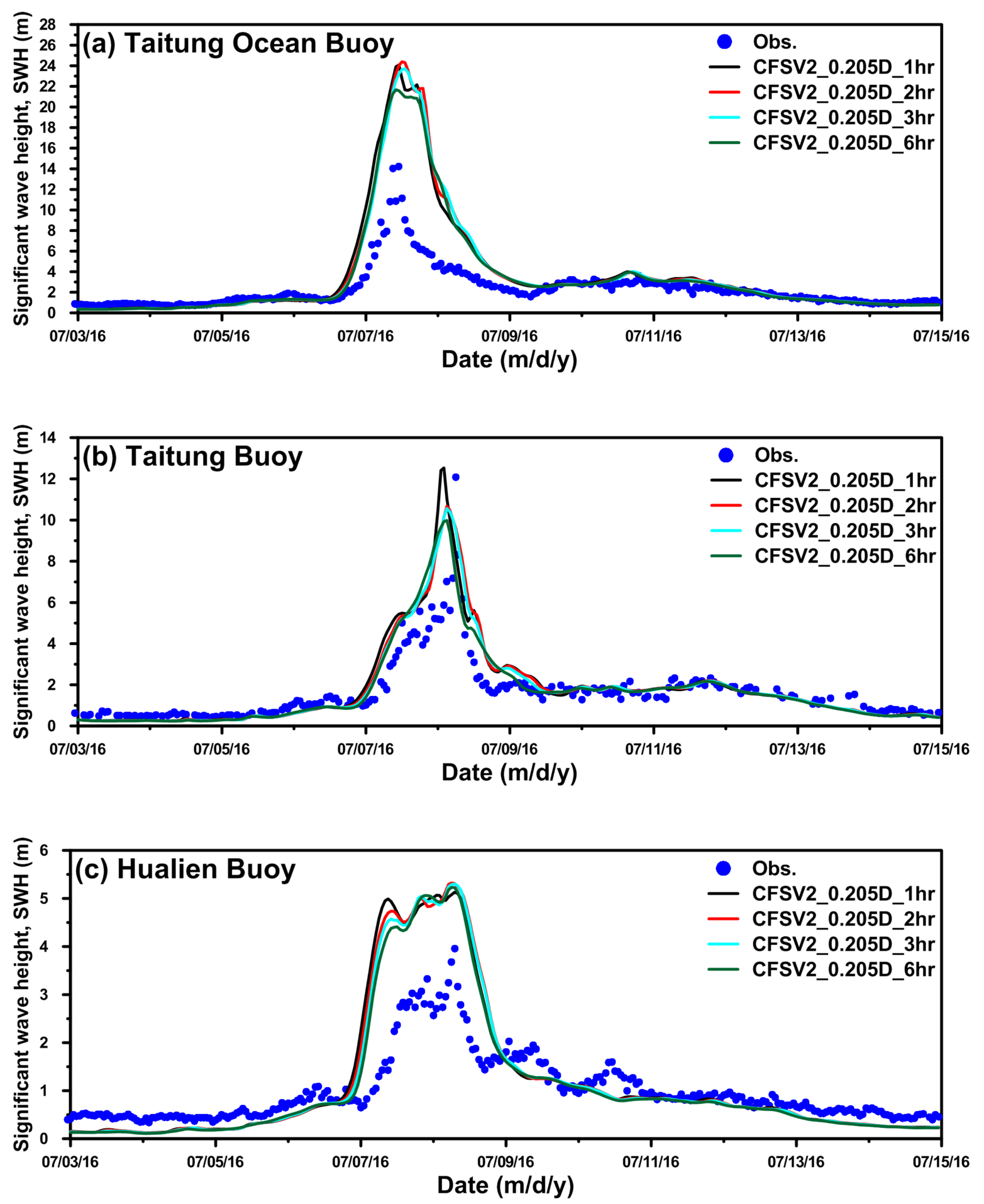
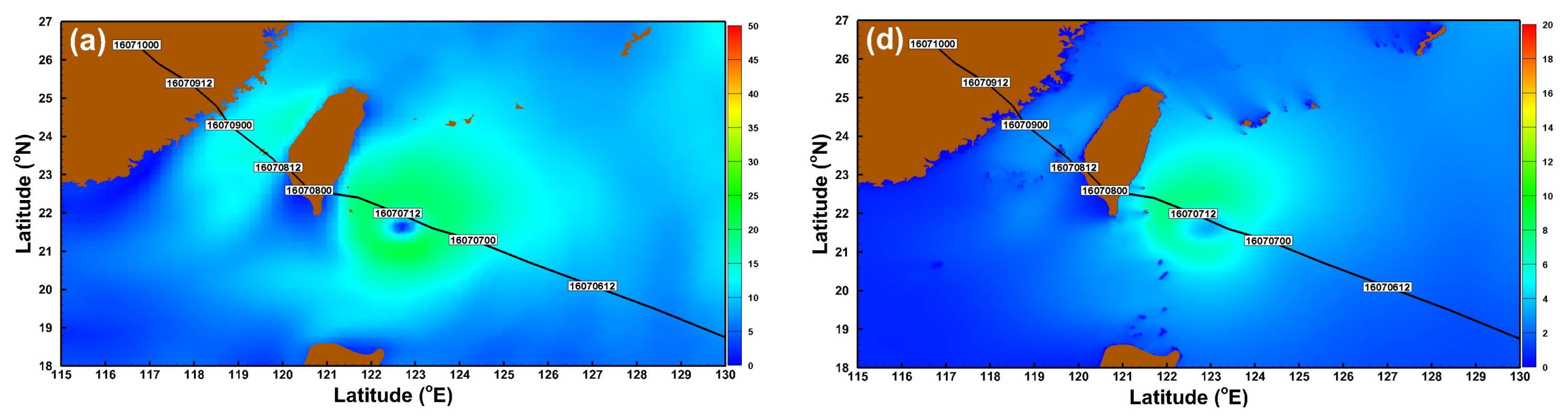
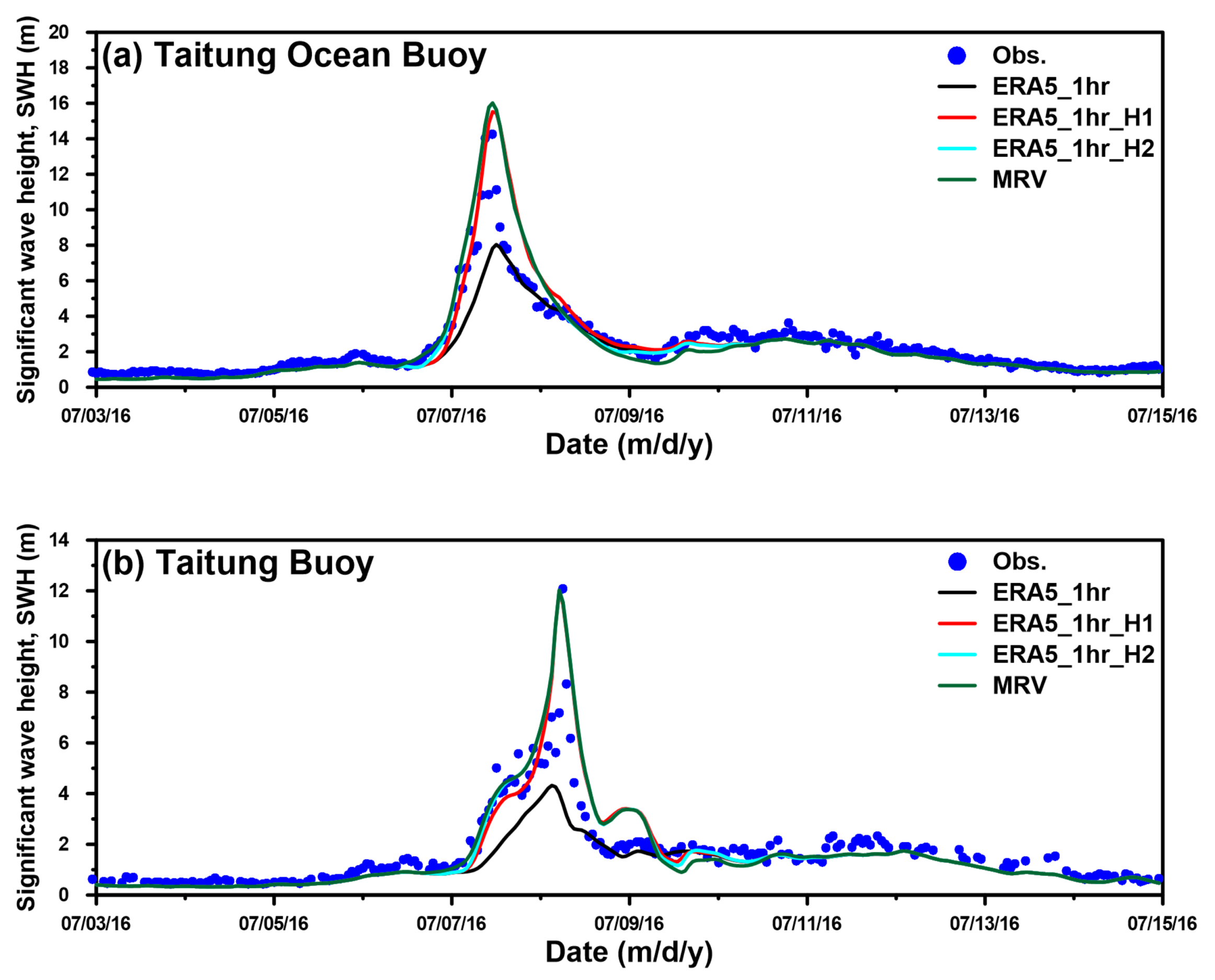
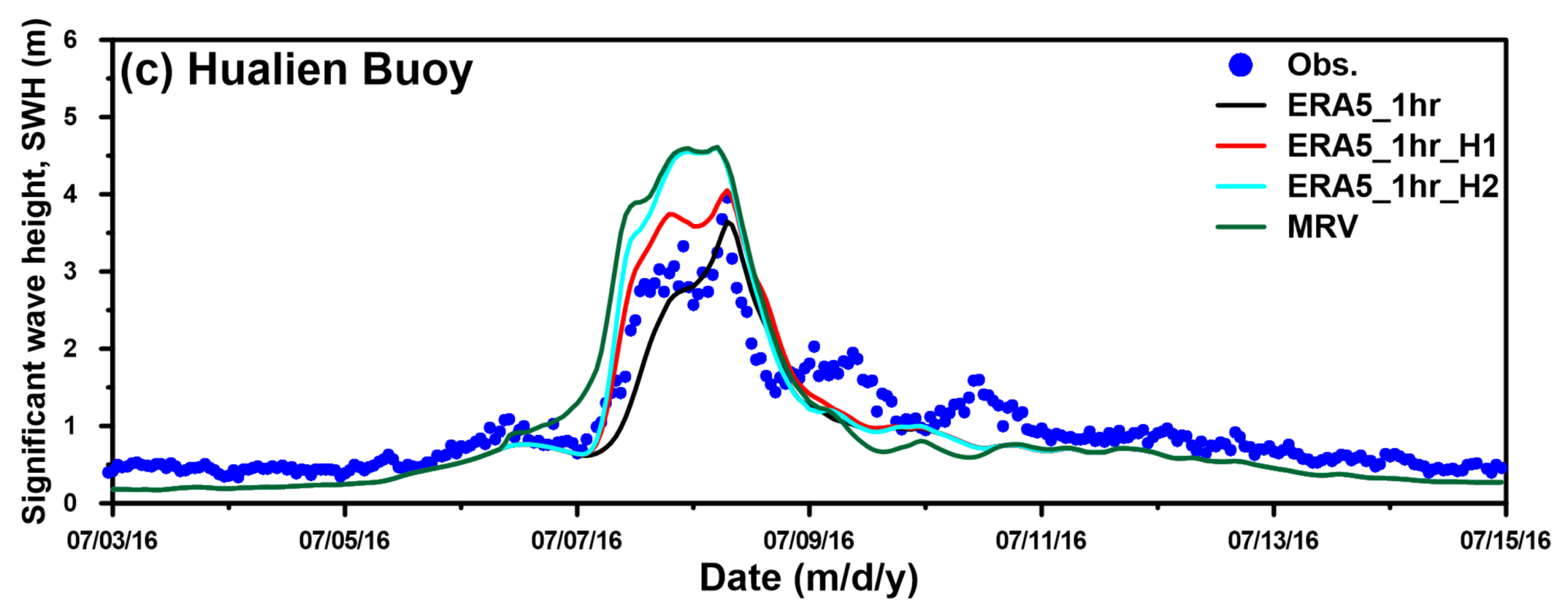
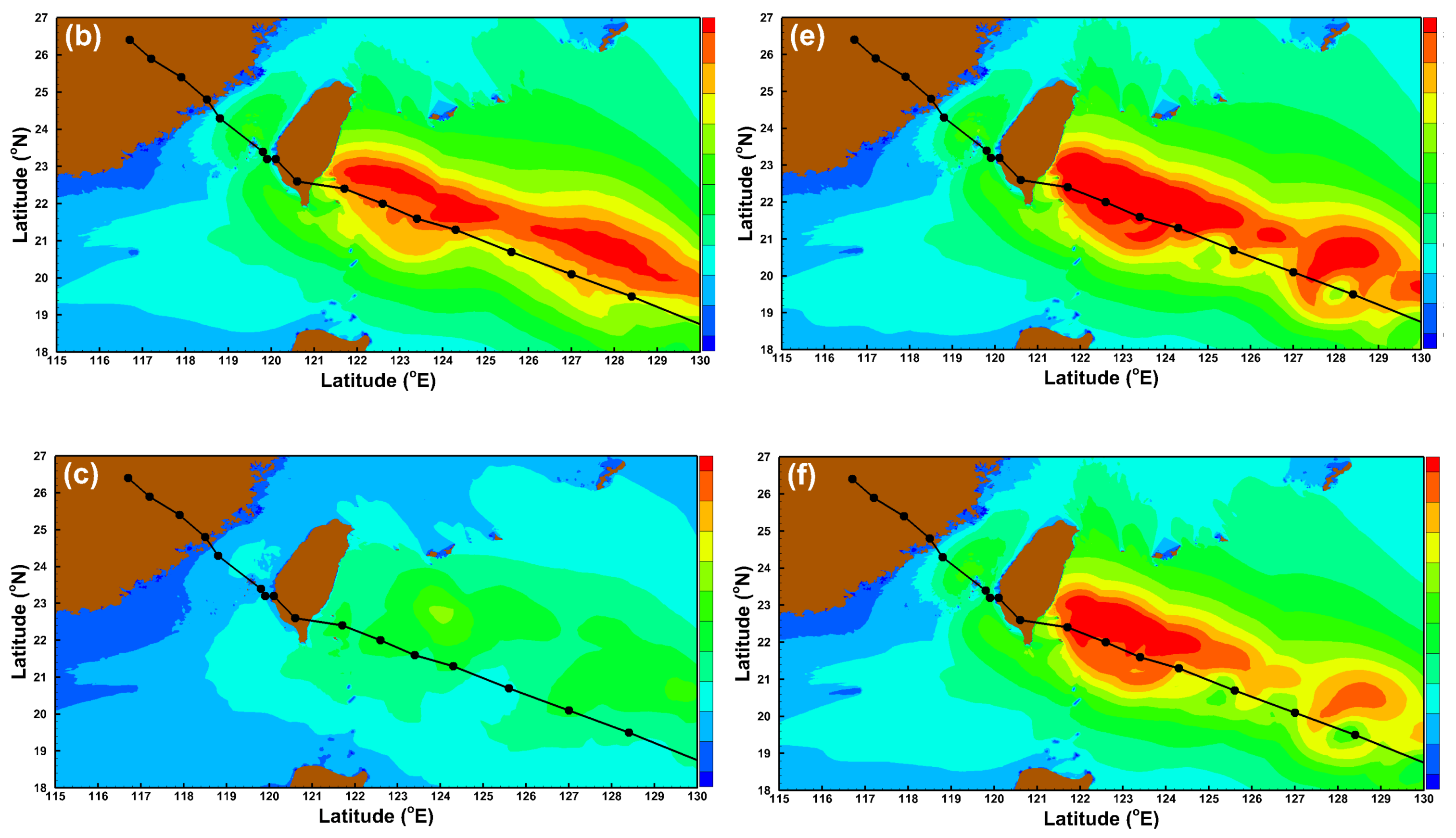
3.2. Effects of the Temporal Resolutions of Wind Fields on Storm Wave Simulation

To better understand the effects of wind temporal resolutions on wave modeling performance, wind fields from CFSV2 with a spatial resolution of 0.205° and temporal resolutions of 1, 2, 3, and 6 h were utilized for reproducing the SWHs during Super Typhoon Nepartak (2016). The instantaneous wind field distributions from CFSV2 with the same spatial resolution (0.205°) and different temporal resolutions are depicted in Figure 6a–d for temporal resolutions of 1, 2, 3, and 6 h, respectively. The variations in wind field from higher to lower temporal resolutions are insignificant except for a delay in time. Figure 6e–h expresses the distributions of simulated instantaneous SWHs corresponding to Figure 6a–d. The patterns of storm waves are insensitive to variations in the wind temporal resolution. Figure 7a–c shows the comparisons of the SWH time series between the modeled and measured values for the Taitung Ocean (Figure 7a), Taitung (Figure 7b), and Hualien (Figure 7c) buoys using winds from the 0.205° CFSV2 with different temporal resolutions. The comparisons shown in Figure 7a–c are dissimilar to those in Figure 5a–c. The storm wave simulations from different wind temporal resolutions are almost identical, except that a 2-m difference was present at the Taitung buoy if the spatial resolution of the wind field remained unchanged.

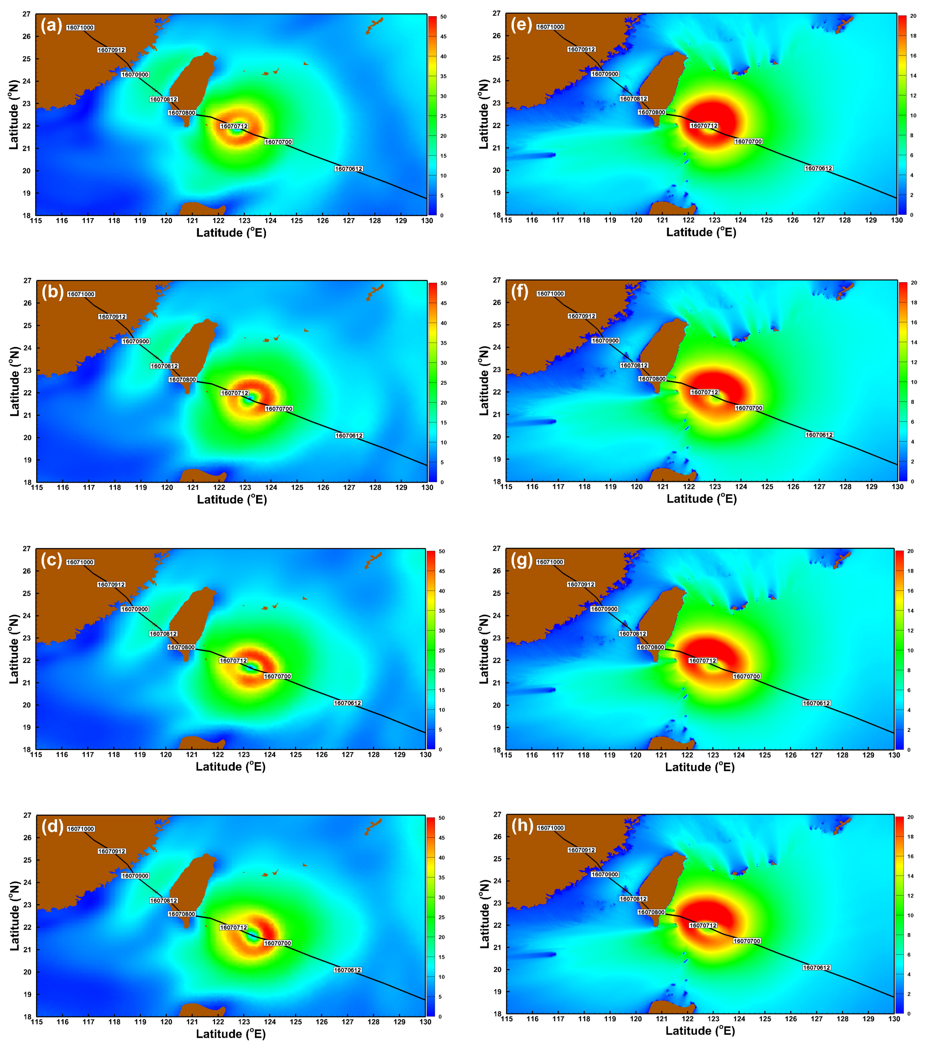
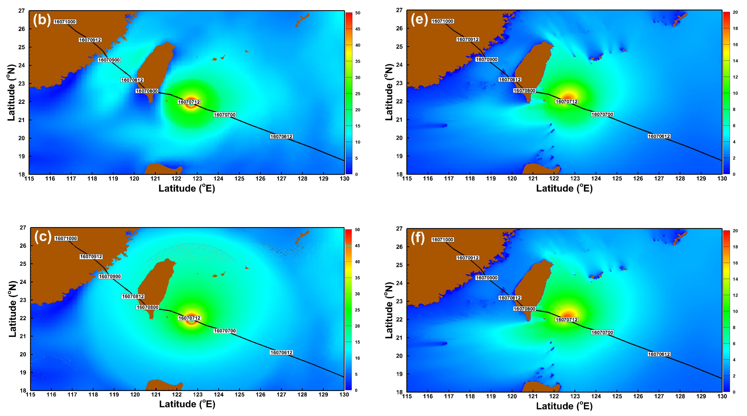
3.3. Effects of Hybrid Wind Fields on Storm Wave Simulation Through Different Superposed Techniques

Although the storm wave heights were overestimated using atmospheric forcing from the hourly CFSV2 with a spatial resolution of 0.205° (hereafter CFSV2_0.025D_1hr), CFSV2_0.025D_1hr could produce a more acceptable wind field distribution. Hence, the SWH computations were again calculated by employing the wind fields derived from merging CFSV2_0.025D_1hr and the MRV typhoon model by means of Equation (4) (hereafter CFSV2_0.025D_1hr_H1) and Equation (7) (hereafter CFSV2_0.025D_1hr_H2). The instantaneous wind field distributions from CFSV2_0.025D_1hr, CFSV2_0.205D_1hr_H1 and CFSV2_0.205D_1hr_H2 are represented in Figure 8a–c. As shown in Figure 8b,c, the region with the higher wind speed (45–50 m/s) decreased and was more concentrated around the center of Super Typhoon Nepartak (2016). Figure 8d–f illustrates the spatial distributions of the SWH reflecting wind forcing from CFSV2_0.025D_1hr, CFSV2_0.205D_1hr_H1 and CFSV2_0.205D_1hr_H2. The extent of extreme waves (16–20 m) decreased, which is particularly true when utilizing winds from CFSV2_0.205D_1hr_H2 (Figure 8f). Figure 9a–c clarifies the improvements in the SWH simulations using the hybrid typhoon winds for the Taitung Ocean (Figure 9a), Taitung (Figure 9b), and Hualien (Figure 9c) buoys. A mismatch between the computed and measured maximum SWH could be reduced from over 9 m to less than 2 m at the Taitung Ocean buoy for Super Typhoon Nepartak (2016).
The hourly reanalysis winds with a spatial resolution of 0.25° (hereafter ERA5_1hr) during Super Typhoon Nepartak (2016) obtained from the ECMWF were also blended with the MRV typhoon model via Equation (4) (hereafter ERA5_1hr_H1) and Equation (7) (hereafter ERA5_1hr_H2). Three wind fields were imposed on the SCHISM-WWM-III to reconfirm that the use of hybrid typhoon winds will greatly improve the storm wave height simulations. Similar to Figure 8a–f, the instantaneous wind fields of ERA5_1hr, ERA5_1hr_H1 and ERA5_1hr_H2 and their corresponding SWH distributions are displayed in Figure 10a–f. The wind speeds of the original ERA5_1hr for Super Typhoon Nepartak (2016) were extremely weak (<30 m/s, as shown in Figure 10a) and consequently led to a smaller storm wave height (<10 m, as shown in Figure 10d). The SWHs of Super Typhoon Nepartak (2016) driven by ERA5_1hr winds were even smaller than those induced by hourly CFSV2 winds with a spatial resolution of 1.875° (as shown green lines in Figure 5a–c). Exerting higher speed winds from ERA5_1hr_H1 and ERA5_1hr_H2 (40–45 m/s, as shown in Figure 10b,c) on SCHISM-WWM-III could cause larger storm waves (approximately 16 m, as shown in Figure 10e,f). Figure 11a–c depicts a comparison of the SWH time series between the simulations and measurements for the Taitung Ocean, Taitung, and Hualien buoys. Introducing a combination of the MRV typhoon wind and reanalysis product into a wave-circulation model significantly enhances the storm wave simulations in both the inner (Figure 11a,b) and outer (Figure 11c) regions of the typhoon. However, ERA5_1hr_H1 resulted in better SWH simulations than ERA5_1hr_H2 for the Hualien buoy (Figure 11c).

4. Discussion

The numerical experiments conducted in the present study show that the storm wave height simulations in both nearshore and offshore areas benefit from inputting the integrations of CFSV2 or ERA5 winds with the MRV typhoon model. The statistical analysis was implemented to quantify the simulation errors when using the CFSV2_0.205D_1hr_H2 and ERA5_1hr_H1 winds during Super Typhoon Nepartak (2016). Table 2 lists the SWH statistical parameters based on a model-data comparison for the Taitung Ocean, Taitung, and Hualien buoys, adopting winds from CFSV2_0.205D_1hr_H2. The minimum SI and HH and the maximum CC are 0.47, 0.32, and 0.97 for the Taitung Ocean buoy, while the maximum SI and HH and the minimum CC are 0.61, 0.45, and 0.92 for the Hualien buoy, respectively. The same statistical parameters are also listed in Table 3 for the utilization of winds from ERA5_1hr_H1. The overall performance of SWH simulations by the ERA5_1hr_H1 winds is slightly better than that by the CFSV2_0.205D_1hr_H2 winds. Figure 12a–f describes the scatter plots of computed SWHs versus measured SWHs for the Taitung Ocean (Figure 12a,d), Taitung (Figure 12b,e), and Hualien (Figure 12c,f) buoys with wind forcing from CFSV2_0.205D_1hr_H2 (Figure 12a–c) and ERA5_1hr_H1 (Figure 12d–f). The larger difference (simulation minus measurement range of 4–6 m) between the measurement of 7–11 m is detected at the Taitung Ocean and Taitung Buoys, as the differences are always less than 4 m at the Hualien Buoy. Table 4 and Table 5 summarize the percentage of model-data difference for different classes and buoys due to the introduction of winds from CFSV2_0.205D_1hr_H2 and ERA5_1hr_H1, respectively. The maximum percentage with a model-data difference larger than 2 m is only 3.03% (2.27% + 0.76%, as shown Table 5) for the Taitung buoy using the ERA5_1hr_H1 winds. Thus, the ERA5_1hr_H1 wind served as an optimal meteorological forcing for simulating SWHs by the SCHISM-WWM-II for Super Typhoon Nepartak (2016).
The SWH simulations driven by winds at a lower resolution are inferior to those generated by winds at a higher resolution. This phenomenon is particularly sensitive to variations in spatial resolution. The spatial distributions of the maximum SWH simulations for Super Typhoon Nepartak (2016) utilizing winds from the hourly CFSV2 with different spatial resolutions and from the CFSV2 with a spatial resolution of 0.205° and different temporal resolutions are illustrated in Figure 13a–f. The maximum SWHs attenuated obviously when the spatial resolution of the wind field was reduced from 0.205° to 1.875° (as shown in Figure 13a–c). The variations in the maximum SWH distribution are relatively small, even if the temporal resolution of the wind fields varies from hourly to 6 h (Figure 13a,d–f); moreover, the discrete maximum SWH distributions are more visible at a lower temporal resolution in the deep ocean (Figure 13e,f). Rusu et al. [51] and Van Vledder and Akpınar [52] suggested that the employment of winds with a higher spatial (mesh) resolution could improve not only typhoon wind filed but also the parameters resulting from the wave model in addition to the SWH. The statistical errors, such as bias, scatter index, and root-mean-square error, for the “SWH” and “spectral period” were usually decrease when the spatial resolution of wind is increased [52]. However, Rusu et al. [51] also recommended that the utilization of winds with a spatial resolution of 4.1 km (approximate 0.04°) is sufficient for simulating wind waves. Adopting winds in a very-high-spatial-resolution (e.g., 0.03°) atmospheric model is the best way to predict, simulate, or hindcast sea states; however, the computing demand increases. Therefore, the next best alternative is the use of a wind field resulting from the superposition of a moderate-spatial-resolution (e.g., 0.2°) atmospheric model and a parametric typhoon model.
Even though modeled and observed wind speed (at 10 m height above sea level) comparisons were implemented in many previous studies [5,48,51,52], the similar comparisons are difficult to conduct in the present study directly. This is because the anemometer on the Taitung Ocean, Taitung, and Hualien buoys is only 2 m above the sea level according to the report from the CWB of Taiwan. The simulations and measurements of wave direction and mean wave period were compared in order to reconfirm the efficiency of the hybrid typhoon winds for improving the wave parameters simulation. Figure 14 shows a model-data comparison for the wave direction (Figure 14a–c) and mean wave period (Figure 14d–f) at different wave buoys. The wave direction and mean wave period simulations were improved using the hybrid typhoon winds, which is particularly true for the mean wave period simulations when winds from ERA5_1hr_H1 were exerted on the SCHISM-WWM-III. Additionally, the storm wave heights from Super Typhoon Nepartak (2016) were simulated with the MRV model alone. As shown in Figure 11a–c (green lines), the utilization of the MRV winds matched the peak SWHs well in the inner region of the typhoon (Figure 11a,b for Taitung Ocean and Taitung buoys) but overestimated the SWHs in outer regions of the typhoon (Figure 11c for Hualien buoy).

5. Summary and Conclusions

In this study, winds from a global atmospheric product, CFSV2, and a global atmospheric reanalysis product, ERA5, as well as winds from a combination of the parametric typhoon model with CFSV2 and ERA5 via two hybrid methods (Equations (4) and (7)), were used as meteorological conditions for a coupled wave-circulation model called SCHISM-WWM-III. The time series of simulated SWHs during Super Typhoon Nepartak (2016) were compared with the observations measured at three wave buoys in the eastern waters of Taiwan. The storm wave heights were severely overestimated due to the presence of hourly CFSV2 winds with a spatial resolution of 0.205°. The hourly CFSV2 wind fields with spatial resolutions of 0.205°, 0.5°, and 1.875° were imposed on the SCHISM-WWM-III. The winds with a coarser spatial resolution usually generated the smaller SWHs. The sensitivity of the temporal resolution of the wind field to the storm wave height simulation was also examined by adopting CFSV2 winds with a spatial resolution of 0.205° and temporal resolutions of 1, 2, 3, and 6 h. However, the simulated SWHs were insensitive to the temporal resolution of wind.
The hourly ERA5 winds with a spatial resolution of 0.25° were applied to the wave-circulation model. Wind speeds acquired from ERA5 in the inner region of Super Typhoon Nepartak (2016) were extremely weak and therefore drove the storm wave heights by only half of the measurements. To overcome the overestimation or underestimation of storm wave height simulations, hybrid typhoon winds were proposed by blending parametric typhoon models (the MRV model) and hourly CFSV2 and ERA5 with spatial resolutions of 0.205° and 0.25°, respectively, by means of two methods. The results demonstrate that using the wind fields derived from the hourly CFSV2 merged with the MRV via Equation (7) could improve the simulations of large storm wave heights close to the track of Super Typhoon Nepartak (2016) but still overestimate the wave heights in the far field of the typhoon. The computed typhoon-generated large SWHs increased significantly, especially for the inner regions of the typhoon, due to the employment of hybrid winds from the hourly ERA5 incorporated with the MRV through Equation (4). Additionally, the timings of the peak SWHs, wave direction and mean wave period during Super Typhoon Nepartak (2016) could also be corrected and well matched by utilizing hybrid wind fields.
Although this study provides insight into the spatial resolution of the CFSV2 wind being more important than the temporal resolution for SWH modeling, a reasonable distribution of typhoon-induced maximum SWHs was created by introducing a wind field with a higher temporal resolution to the SCHISM-WWM-III. Using the hybrid wind fields from CFSV2 and ERA5 produced similar storm wave heights near the track of Super Typhoon Nepartak (2016); however, the simulations of storm wave height agreed well with the observations in both the near and far fields of typhoon by applying the blended winds from ERA5 only, which is particularly essential for successful storm wave computation. The findings of this study will greatly benefit the accuracy of the operational marine weather forecast system, the design of infrastructure in nearshore waters, and the prevention of coastal disasters. Moreover, the combination of a numerical atmospheric or reanalysis product with higher spatial and temporal resolutions with parametric typhoon winds is the optimal atmospheric condition for a coupled wave-circulation model to predict or hindcast storm wave height accurately.

Author Contributions

Conceptualization, S.-C.H., H.C., H.-L.W., W.-B.C., C.-H.C., W.-D.G. and L.-Y.L. Methodology, W.-B.C. and H.-L.W. Validation, W.-B.C. Formal analysis, H.-L.W., C.-H.C., W.-D.G. and Y.-M.C. Writing—original draft preparation, W.-B.C., S.-C.H., H.-L.W. and L.-Y.L. Supervision, S.-C.H., H.C. and L.-Y.L. All authors have read and agreed to the published version of the manuscript.

Funding

This research was funded by the Ministry of Science and Technology (MOST), Taiwan, grant No. MOST 108-2625-M-865-001.

Acknowledgments

The authors would like to thank the Central Weather Bureau and Department of Land Administration, Ministry of the Interior of Taiwan for providing the measured data as well as Joseph Zhang at the Virginia Institute of Marine Science, College of William & Mary, and Aron Roland at the BGS IT&E GmbH, Darmstadt, Germany, for kindly sharing their experiences concerning the use of the numerical model.

Conflicts of Interest

The authors declare no conflict of interest.

References

  1. Shao, Z.; Liang, B.; Li, H.; Wu, G.; Wu, Z. Blended wind fields for wave modeling of tropical cyclones in the South China Sea and East China Sea. Appl. Ocean Res. 2018, 71, 20–33. [Google Scholar] [CrossRef]
  2. Shih, H.-J.; Chang, C.-H.; Chen, W.-B.; Lin, L.-Y. Identifying the Optimal Offshore Areas for Wave Energy Converter Deployments in Taiwanese Waters Based on 12-Year Model Hindcasts. Energies 2018, 11, 499. [Google Scholar] [CrossRef] [Green Version]
  3. Chang, C.-H.; Shih, H.-J.; Chen, W.-B.; Su, W.-R.; Lin, L.-Y.; Yu, Y.-C.; Jang, J.-H. Hazard Assessment of Typhoon-Driven Storm Waves in the Nearshore Waters of Taiwan. Water 2018, 10, 926. [Google Scholar] [CrossRef] [Green Version]
  4. Chen, W.-B.; Chen, H.; Hsiao, S.-C.; Chang, C.-H.; Lin, L.-Y. Wind forcing effect on hindcasting of typhoon-driven extreme waves. Ocean Eng. 2019, 188, 106260. [Google Scholar] [CrossRef]
  5. Murty, P.N.L.; Srinivas, K.S.; Rao Rama Pattabhi, E.; Bhaskaran, P.K.; Shenoi, S.S.C.; Padmanabham, J. Improved cyclone wind fields over the Bay of Bengal and their application in storm surge and wave computations. Appl. Ocean Res. 2020, 95, 102048. [Google Scholar] [CrossRef]
  6. Huang, F.; Xu, S. Super typhoon activity over the western North Pacific and its relationship with ENSO. J. Ocean Univ. China 2010, 9, 123–128. [Google Scholar] [CrossRef]
  7. Balaguru, K.; Foltz, G.R.; Leung, L.R.; Emanuel, K.A. Global warming-induced upper-ocean freshening and the intensification of super typhoons. Nat. Commun. 2016, 7, 13670. [Google Scholar] [CrossRef] [PubMed] [Green Version]
  8. Akpınar, A.; Bingölbali, B.; van Vledder, G.P. Wind and wave characteristics in the Black Sea based on the SWAN wave model forced with the CFSR winds. Ocean Eng. 2016, 126, 276–298. [Google Scholar] [CrossRef]
  9. Kim, E.; Manuel, L.; Curcic, M.; Chen, S.S.; Phillips, C.; Veers, P. On the Use of Coupled Wind, Wave, and Current Fields in the Simulation of Loads on Bottom Supported Offshore Wind Turbines during Hurricanes; Technical Report NREL/TP-5000-65283; National Renewable Energy Laboratory: Golden, CO, USA, 2016. [Google Scholar]
  10. Li, X.; Chen, Y.; Pan, S.; Pan, Y.; Fang, J.; Sowa, D.M.A. Estimation of mean and extreme waves in the East China Seas. Appl. Ocean Res. 2016, 56, 35–47. [Google Scholar] [CrossRef]
  11. Osorio, A.F.; Montoya, R.D.; Ortiz, J.C.; Peláez, D. Construction of synthetic ocean wave series along the Colombian Caribbean Coast: A wave climate analysis. Appl. Ocean Res. 2016, 56, 119–131. [Google Scholar] [CrossRef]
  12. Orimolade, A.P.; Haver, S.; Gudmestad, O.T. Estimation of extreme significant wave heights and the associated uncertainties: A case study using NORA10 hindcast data for the Barents Sea. Mar. Struct. 2016, 49, 1–17. [Google Scholar] [CrossRef]
  13. Muraleedharan, G.; Lucas, C.; Soares, C.G. Regression quantile models for estimating trends in extreme significant wave heights. Ocean Eng. 2016, 118, 204–215. [Google Scholar] [CrossRef]
  14. Lau, A.Y.A.; Terry, J.P.T.; Ziegler, A.D.; Switzer, A.D.; Lee, Y.; Etienne, S. Understanding the history of extreme wave events in the Tuamotu Archipelago of French Polynesia from large carbonate boulders on Makemo Atoll, with implications for future threats in the central South Pacific. Mar. Geol. 2016, 380, 174–190. [Google Scholar] [CrossRef]
  15. Hsiao, S.-C.; Chen, H.; Chen, W.-B.; Chang, C.-H.; Lin, L.-Y. Quantifying the contribution of nonlinear interactions to storm tide simulations during a super typhoon event. Ocean Eng. 2019, 194, 106661. [Google Scholar] [CrossRef]
  16. Zhang, Y.J.; Ye, F.; Stanev, E.V.; Grashorn, S. Seamless cross-scale modelling with SCHISM. Ocean Model. 2016, 102, 64–81. [Google Scholar] [CrossRef] [Green Version]
  17. Zhang, Y.J.; Baptista, A.M. SELFE: A semi-implicit Eulerian-Lagrangian finite-element model for cross-scale ocean circulation. Ocean Model. 2008, 21, 71–96. [Google Scholar] [CrossRef]
  18. Shchepetkin, A.F.; McWilliams, J.C. The regional oceanic modeling system (ROMS): A split-explicit, free-surface, topography-following-coordinate, oceanic model. Ocean Model. 2005, 9, 347–404. [Google Scholar] [CrossRef]
  19. Wang, H.V.; Loftis, J.D.; Liu, Z.; Forrest, D.; Zhang, J. The storm surge and sub-grid inundation modeling in New York City during hurricane Sandy. J. Mar. Sci. Eng. 2014, 1, 226–246. [Google Scholar] [CrossRef] [Green Version]
  20. Chen, W.-B.; Liu, W.-C. Modeling flood inundation Induced by river flow and storm surges over a river basin. Water 2014, 6, 3182–3199. [Google Scholar] [CrossRef] [Green Version]
  21. Chen, W.-B.; Liu, W.-C. Assessment of storm surge inundation and potential hazard maps for the southern coast of Taiwan. Nat. Hazards 2016, 82, 591–616. [Google Scholar] [CrossRef]
  22. Chen, W.-B.; Chen, H.; Lin, L.-Y.; Yu, Y.-C. Tidal Current Power Resource and Influence of Sea-Level Rise in the Coastal Waters of Kinmen Island, Taiwan. Energies 2017, 10, 652. [Google Scholar] [CrossRef] [Green Version]
  23. Chen, Y.-M.; Liu, C.-H.; Shih, H.-J.; Chang, C.-H.; Chen, W.-B.; Yu, Y.-C.; Su, W.-R.; Lin, L.-Y. An Operational Forecasting System for Flash Floods in Mountainous Areas in Taiwan. Water 2019, 11, 2100. [Google Scholar] [CrossRef] [Green Version]
  24. Komen, G.J.; Cavaleri, L.; Donelan, M.; Hasselmann, K.; Hasselmann, S.; Janssen, P.A.E. Dynamics and Modelling of Ocean Waves; Cambridge University Press: Cambridge, UK, 1994; p. 532. [Google Scholar]
  25. Roland, A. Development of WWM II: Spectral Wave Modeling on Unstructured Meshes. Ph.D. Thesis, Technology University Darmstadt, Darmstadt, Germany, 2009. [Google Scholar]
  26. Yanenko, N.N. The Method of Fractional Steps; Springer: Berlin/Hamburg, Germany, 1971. [Google Scholar]
  27. Hasselmann, K.; Barnett, T.P.; Bouws, E.; Carlson, H.; Cartwright, D.E.; Enke, K.; Ewing, J.A.; Gienapp, H.; Hasselmann, D.E.; Kruseman, P.; et al. Measurements of Wind-Wave Growth and Swell Decay during the Joint North Sea Wave Project (JONSWAP); Deutsches Hydrographisches Institut: Berlin/Hamburg, Germany, 1973. [Google Scholar]
  28. Roland, A.; Zhang, Y.J.; Wang, H.V.; Meng, Y.; Teng, Y.-C.; Maderich, V.; Brovchenko, I.; Dutour-Sikiric, M.; Zanke, U. A fully coupled 3D wave-current interaction model on unstructured grids. J. Geophys. Res. 2012, 117, C00J33. [Google Scholar] [CrossRef]
  29. Zhang, H.; Sheng, J. Estimation of extreme sea levels over the eastern continental shelf of North America. J. Geophys. Res. Oceans 2013, 118, 6253–6273. [Google Scholar] [CrossRef]
  30. Muis, S.; Verlaan, M.; Winsemius, H.C.; Aerts, J.C.J.H.; Ward, P.J. A global reanalysis of storm surges and extreme sea levels. Nat. Commun. 2016, 7, 11969. [Google Scholar] [CrossRef] [PubMed] [Green Version]
  31. Marsooli, R.; Lin, N. Numerical Modeling of Historical Storm Tides and Waves and Their Interactions Along the U.S. East and Gulf Coasts. J. Geophys. Res. Oceans 2018, 123, 3844–3874. [Google Scholar] [CrossRef] [Green Version]
  32. Zu, T.; Gana, J.; Erofeevac, S.Y. Numerical study of the tide and tidal dynamics in the South China Sea. Deep Sea Res. 2008, 55, 137–154. [Google Scholar] [CrossRef]
  33. Saha, S.; Moorthi, S.; Wu, X.; Wang, J.; Nadiga, S.; Tripp, P.; Pan, H.-L.; Behringer, D.; Hou, Y.-T.; Chuang, H.-Y.; et al. The NCEP Climate Forecast System Version 2. J. Clim. 2014, 27, 2185–2208. [Google Scholar] [CrossRef]
  34. Fujita, T. Pressure distribution within typhoon. Geophys. Mag. 1952, 23, 437–451. [Google Scholar]
  35. Jelesnianski, C.P. A numerical computation of storm tides induced by a tropical storm impinging on a continental shelf. Mon. Weather Rev. 1965, 93, 343–358. [Google Scholar] [CrossRef] [Green Version]
  36. Holland, G.J. An analytical model of the wind and pressure profiles in hurricanes. Mon. Weather Rev. 1980, 108, 1212–1218. [Google Scholar] [CrossRef]
  37. Phadke, A.C.; Martino, C.D.; Cheung, K.F.; Houston, S.H. Modeling of tropical cyclone winds and waves for emergency management. Ocean Eng. 2003, 30, 553–578. [Google Scholar] [CrossRef]
  38. Wang, X.; Qian, C.; Wang, W.; Yan, T. An elliptical wind field model of typhoons. J. Ocean Univ. China 2004, 3, 33–39. [Google Scholar] [CrossRef]
  39. MacAfee, A.W.; Pearson, G.W. Development and testing of tropical Cyclone parametric wind models tailored for midlatitude application-preliminary results. J. Appl. Meteorol. Climatol. 2006, 45, 1244–1260. [Google Scholar] [CrossRef]
  40. Wood, V.T.; White, L.W.; Willoughby, H.E.; Jorgensen, D.P. A new parametric tropical cyclone tangential wind profile model. Mon. Weather Rev. 2013, 141, 1884–1909. [Google Scholar] [CrossRef]
  41. Cheung, K.F.; Tang, L.; Donnelly, J.P.; Scileppi, E.M.; Liu, K.B.; Mao, K.B.; Houston, S.H.; Murnane, R.J. Numerical modeling and field evidence of coastal overwash in southern New England from Hurricane Bob and implications for paleotempestology. J. Geophys. Res. 2007, 112, F03024. [Google Scholar] [CrossRef] [Green Version]
  42. Bastidas, L.A.; Knighton, J.; Kline, S.W. Parameter sensitivity and uncertainty analysis for a storm surge and wave model. Nat. Hazards Earth Syst. Sci. 2016, 16, 2195–2210. [Google Scholar] [CrossRef] [Green Version]
  43. Tolman, H.L.; Alves, J.H.G.M. Numerical modeling of waves generated by tropical cyclones using moving grids. Ocean Model. 2005, 9, 305–323. [Google Scholar] [CrossRef]
  44. Yu, Y.-C.; Chen, H.; Shih, H.-J.; Chang, C.-H.; Hsiao, S.-C.; Chen, W.-B.; Chen, Y.-M.; Su, W.-R.; Lin, L.-Y. Assessing the Potential Highest Storm Tide Hazard in Taiwan Based on 40-year Historical Typhoon Surge Hindcasting. Atmosphere 2019, 10, 346. [Google Scholar] [CrossRef] [Green Version]
  45. Atkinson, G.D.; Holliday, C.R. Tropical cyclone minimum sea level pressure/maximum sustained wind relationship for the western North Pacific. Mon. Weather. Rev. 1977, 105, 421–427. [Google Scholar] [CrossRef] [Green Version]
  46. Pan, Y.; Chen, Y.P.; Li, J.X.; Ding, X.L. Improvement of wind field hindcasts for tropical cyclones. Water Sci. Eng. 2016, 9, 58–66. [Google Scholar] [CrossRef] [Green Version]
  47. Li, J.; Pan, S.; Chen, Y.; Fan, Y.M.; Pan, Y. Numerical estimation of extreme waves and surges over the northwest Pacific Ocean. Ocean Eng. 2018, 153, 225–241. [Google Scholar] [CrossRef]
  48. Qiao, W.; Song, J.; He, H.; Li, F. Application of different wind filed models and wave boundary layer model to typhoon waves numerical simulation in WAVEWATCH III model. Tellus A 2019, 7, 1657552. [Google Scholar] [CrossRef] [Green Version]
  49. Hanna, S.; Heinold, D. Development and Application of a Simple Method for Evaluating Air Quality; API Pub.: Washington, DC, USA, 1985. [Google Scholar]
  50. Mentaschi, L.; Besio, G.; Cassola, F.; Mazzino, A. Problems in RMSE-based wave model validations. Ocean Model. 2013, 72, 53–58. [Google Scholar] [CrossRef]
  51. Rusu, L.; Bernardino, M.; Guedes Soares, C. Influence of Wind Resolution on Prediction of Waves Generated in an Estuary. J. Coast. Res. 2009, 56, 1419–1423. [Google Scholar]
  52. Van Vledder, G.P.; Akpınar, A. Wave model predictions in the Black Sea: Sensitivity to wind fields. Appl. Ocean Res. 2015, 53, 161–178. [Google Scholar] [CrossRef]
Figure 1. Typhoon-driven storm waves breached a sea wall (upper-right panel) and damaged a lighthouse (lower-left panel) in the southeastern waters of Taiwan (photo by the present study).
Jmse 08 00217 g001
Figure 2. Track and central air pressures of Super Typhoon Nepartak in 2016 and the locations of wave buoys. The color of the solid circles represents the typhoon intensity as classified on the Saffir–Simpson scale (red: category 5; yellow: category 4; green: category 3; cyan: category 2; blue: category 1).
Jmse 08 00217 g002
Figure 3. Entire computational meshes (a), enlargement of high-resolution unstructured grids for the southern coastal waters of Taiwan (b), and bathymetry (c).
Jmse 08 00217 g003
Figure 4. Instantaneous wind field distribution from the hourly Climate Forecast System version 2 (CFSV2) with spatial resolutions of (a) 0.205°, (b) 0.5°, and (c) 1.875° and their corresponding SWHs (df) for Super Typhoon Nepartak at 11:00 on 12 July in 2016.
Jmse 08 00217 g004
Figure 5. Model-data comparison for SWH time series at the (a) Taitung Ocean, (b) Taitung, and (c) Hualien buoys employing the winds from the hourly CFSV2 at different spatial resolutions.
Jmse 08 00217 g005
Figure 6. Instantaneous wind field distribution from CFSV2 with a spatial resolution of 0.205° and temporal resolutions of (a) 1 h, (b) 2 h, (c) 3 h, and (d) 6 h and their corresponding SWHs (eh) during Super Typhoon Nepartak at 11:00 on 12 July in 2016.
Jmse 08 00217 g006
Figure 7. Model-data comparison for the SWH time series of the (a) Taitung Ocean, (b) Taitung, and (c) Hualien buoys employing the winds from CFSV2 with a spatial resolution of 0.205° and different temporal resolutions.
Jmse 08 00217 g007
Figure 8. Instantaneous wind field distribution from the (a) hourly CFSV2 with a spatial resolution of 0.205°, (b) CFSV2_0.205D_1hr_H1, and (c) CFSV2_0.205D_1hr_H2 and their corresponding SWHs (df) for Super Typhoon Nepartak at 11:00 on 12 July in 2016.
Jmse 08 00217 g008
Figure 9. Model-data comparison for the SWH time series the (a) Taitung Ocean, (b) Taitung, and (c) Hualien buoys employing winds from CFSV2 with a spatial resolution of 0.205°, CFSV2_0.205D_1hr_H1, and CFSV2_0.205D_1hr_H2.
Jmse 08 00217 g009
Figure 10. Instantaneous wind field distribution from the (a) hourly ERA5, (b) ERA5_1hr_H1, and (c) ERA5_1hr_H2 and their corresponding SWHs (df) for Super Typhoon Nepartak at 11:00 on 12 July in 2016.
Jmse 08 00217 g010aJmse 08 00217 g010b
Figure 11. Model-data comparison for the SWH time series at the (a) Taitung Ocean, (b) Taitung, and (c) Hualien buoys employing the winds from ERA5_1hr, ERA5_1hr_H1, ERA5_1hr_H2, and modified Rankine vortex (MRV).
Jmse 08 00217 g011aJmse 08 00217 g011b
Figure 12. Scatter plot of computed versus measured SWHs at the (a,d) Taitung Ocean, (b,e) Taitung, and (c,f) Hualien buoys employing the winds from CFSV2_0.205D_1hr_H2 (ac) and ERA5_1hr_H1 (df).
Jmse 08 00217 g012aJmse 08 00217 g012b
Figure 13. Spatial distribution of maximum SWHs driven by winds from the hourly CFSV2 with spatial resolutions of (a) 0.205°, (b) 0.5°, and (c) 1.875° and from CFSV2 with a spatial resolution of 0.205° and temporal resolutions of (d) 2 h, (e) 3 h, and (f) 6 h for Super Typhoon Nepartak in 2016.
Jmse 08 00217 g013aJmse 08 00217 g013b
Figure 14. Model-data comparison for the wave direction (ac) and mean wave period (df) time series at the (a,d) Taitung Ocean, (b,e) Taitung, and (c,f) Hualien buoys employing the winds from CFSV2_0.205D_1hr, ERA5_1hr, CFSV2_0.205D_1hr_H2, and ERA5_1hr_H1.
Jmse 08 00217 g014
Table 1. Information on wave buoys.
Buoy NameLongitude (°E)Latitude (°N)Water Depth (m)
Taitung Ocean124.074221.76645610
Taitung121.145022.724030
Hualien121.631424.031921
Data source: The CWB of Taiwan.
Table 2. Statistical parameters of SWH based on model-data comparison for different buoys using winds from CFSV2_0.205D_1hr_H2.
Buoy NameSICCHH
Taitung Ocean0.470.970.32
Taitung0.500.940.33
Hualien0.610.920.45
Table 3. Statistical parameters of SWH based on model-data comparison for different buoys using winds from ERA5_1hr_H1.
Buoy NameSICCHH
Taitung Ocean0.390.960.28
Taitung0.390.920.35
Hualien0.360.950.31
Table 4. Percentage of model-data difference for different classes and buoys using winds from CFSV2_0.205D_1hr_H2.
Buoy Name[−2,0)[0,2)[2,4)[4,6)
Taitung Ocean67.4826.294.341.90
Taitung64.0232.952.270.76
Hualien85.1213.771.100.00
Table 5. Percentage of model-data difference for different classes and buoys using winds from ERA5_1hr_H1.
Buoy Name[−2,0)[0,2)[2,4)[4,6)
Taitung Ocean77.5119.751.081.63
Taitung76.8920.082.270.76
Hualien88.7111.290.000.00

