Numerical Simulation of Volume Change of the Backshore Induced by Cross-Shore Aeolian Sediment Transport


Abstract
:
1. Introduction
2. Study Site and Data Description
2.1. Study Site
2.2. Beach Profile
2.3. Winds
2.4. Rainfall
2.5. Vegetation
3. Methods
3.1. Simulation Model of Backshore Volume Change
3.2. Calibration and Validation
4. Results
4.1. Calibration
4.2. Validation
5. Discussion
6. Conclusions
Author Contributions
Funding
Acknowledgments
Conflicts of Interest
Appendix A. Correcting Missing Wind Data


List of Tables and Figures
| Tables |
| Table 1. The RMS error, the correlation coefficient, and BSS for the weekly averaged volume-change rate and the cumulative volume change in the calibration process. |
| Table 2. The RMS error, the correlation coefficient, and BSS for the weekly averaged volume-change rate and the cumulative volume change in the validation process. |
| Figures |
| Figure 1. Location of study site. |
| Figure 2. Plan view of the study area and the survey line. The contour lines are based on the survey data on 11 November 1996. |
| Figure 3. Mean beach profile and the profiles at the beginning and end of the investigation period from x = −115 to 40 m along the survey line indicated in Figure 2. |
| Figure 4. Temporal variation of the cumulative volume change in the investigation area based on the beach profile measured on 5 January 1987. |
| Figure 5. Coordinate system. |
| Figure 6. Monthly averaged wind characteristics: (a) absolute wind velocity and wind direction and (b) wind-velocity components in cross-shore and alongshore directions. The positive cross-shore and alongshore wind velocities are landward and southward, respectively. |
| Figure 7. Yearly averaged wind characteristics. See Figure 6 for further explanation. Figure 8. Monthly averaged amounts of precipitation. |
| Figure 9. Yearly averaged amounts of precipitation. |
| Figure 10. Photos of vegetation in a square mesh taken on 24 June 1996 (a) and 14 January 1997 (b). |
| Figure 11. Monthly averaged Cveg1. |
| Figure 12. Time series of Cveg2,N and Cveg2,S. |
| Figure 13. Photos of vegetation along and around the survey line taken on 2 August 1995 (a) and 1 June 2007 (b). The broken lines display the survey line. |
| Figure 14. Correlation between the measured and simulated weekly averaged volume-change rates in the calibration process. |
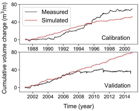
| Figure 15. Time series of the measured and simulated cumulative volume changes in the calibration process. |
| Figure 16. Correlation between the measured and simulated weekly averaged volume-change rates in the validation process. |
| Figure 17. Time series of the measured and simulated cumulative volume changes in the validation process. |
| Figure 18. The cumulative volume changes at the end of the investigation period simulated using the values of K, c1, and c2 that were increased and decreased by 10%. The broken line shows the volume simulated using the best-fit parameter values. |
| Figure 19. Measured and simulated weekly averaged volume-change rates in the calibration process: (a) power spectral densities, (b) coherence, and (c) phase. |
| Figure 20. Measured and simulated weekly averaged volume-change rates in the validation process: (a) power spectral densities, (b) coherence, and (c) phase. |
| Figures in Appendix |
| Figure A1. Correlation between reproduced and measured cross-shore wind velocities. The black line represents the linear correlation estimated by the least-squares method. |
| Figure A2. Correlation between reproduced and measured alongshore wind velocities. The black line represents the linear correlation estimated by the least-squares method. |
References
- Komar, P.D. Beach Processes and Sedimentation, 2nd ed.; Prentice Hall: Englewood Cliffs, NJ, USA, 1998; p. 544. [Google Scholar]
- McLachlan, A. The exchange of materials between dune and beach systems. In Coastal Dunes: Form and Process; Nordstrom, K.F., Psuty, N.P., Carter, R.W.G., Eds.; John Wiley & Sons Ltd.: Chichester, UK, 1990; pp. 202–213. [Google Scholar]
- Brown, A.C.; McLachlan, A. Ecology of Sandy Shores; Elsevier: Amsterdam, The Netherlands, 1990; p. 328. [Google Scholar]
- Van Dijk, P.M.; Arens, S.M.; van Boxel, J.H. Aeolian processes across transverse dunes. II: Modelling the sediment transport and profile development. Earth Surf. Process. Landf. 1999, 24, 319–333. [Google Scholar]
- Luna, M.C.D.M.; Parteli, E.J.; Durán, O.; Herrmann, H.J. Model for the genesis of coastal dune fields with vegetation. Geomorphology 2011, 129, 215–224. [Google Scholar] [CrossRef]
- Durán, O.; Moore, L.J. Vegetation controls on the maximum size of coastal dunes. Proc. Natl. Acad. Sci. USA 2013, 110, 17217–17222. [Google Scholar] [CrossRef] [Green Version]
- Davidson-Arnott, R.G.D.; Hesp, P.; Ollerhead, J.; Walker, I.; Bauer, B.; Delgado-Fernandez, I.; Smyth, T. Sediment Budget Controls on Foredune Height: Comparing Simulation Model Results with Field Data. Earth Surf. Process Landf. 2018, 43, 1798–1810. [Google Scholar] [CrossRef]
- Larson, M.; Palalane, J.; Fredriksson, C.; Hanson, H. Simulating cross-shore material exchange at decadal scale. Theory and model component validation. Coast. Eng. 2016, 116, 57–66. [Google Scholar] [CrossRef]
- Palalane, J.; Fredriksson, C.; Marinho, B.; Larson, M.; Hanson, H.; Coelho, C. Simulating cross-shore material exchange at decadal scale. Model application. Coast. Eng. 2016, 116, 26–41. [Google Scholar] [CrossRef]
- Hallin, C.; Larson, M.; Hanson, H. Simulating beach and dune evolution at decadal to centennial scale under rising sea levels. PLoS ONE 2019, 14, e0215651. [Google Scholar] [CrossRef] [Green Version]
- Cohn, N.; Hoonhout, B.M.; Goldstein, E.B.; de Vries, S. Exploring Marine and Aeolian Controls on Coastal Foredune Growth Using a Coupled Numerical Model. J. Mar. Sci. Eng. 2019, 7, 1–25. [Google Scholar] [CrossRef] [Green Version]
- Roelvink, D.; Reniers, A.A.; van Dongeren, J.; van Thiel de Vries, J.; McCall, R.; Lescinski, J. Modelling storm impacts on beaches, dunes and barrier islands. Coast. Eng. 2009, 56, 1133–1152. [Google Scholar] [CrossRef]
- Hoonhout, B.M.; de Vries, S. A Process-based Model for Aeolian sediment Transport and Spatiotemporal Varying Sediment Availability. J. Geophys. Res. Earth Surf. 2016, 121, 1555–1575. [Google Scholar] [CrossRef]
- Roelvink, D.J.A.; Costas, S. Coupling nearshore and aeolian processes: XBeach and Duna process-based models. Environ. Modell. Softw. 2019, 115, 98–112. [Google Scholar] [CrossRef]
- Davidson-Arnott, R.G.D.; Law, M.N. Seasonal patterns and controls on sediment supply to coastal foredunes, Long Point, Lake Erie. In Coastal Dunes: Form and Process; Nordstrom, K.F., Psuty, N.P., Carter, R.W.G., Eds.; John Wiley & Sons Ltd.: Chichester, UK, 1990; pp. 177–200. [Google Scholar]
- Davidson-Arnott, R.G.D.; Law, M.N. Measurement and prediction of long-term sediment supply to coastal foredunes. J. Coast. Res. 1996, 12, 654–663. [Google Scholar]
- Nordstrom, K.F.; Jackson, N.L. Effect of source width and tidal elevation changes on aeolian transport on an estuarine beach. Sedimentology 1992, 39, 769–778. [Google Scholar] [CrossRef]
- Jackson, D.W.T.; Cooper, A. Beach fetch distance and aeolian sediment transport. Sedimentology 1999, 46, 517–522. [Google Scholar]
- Hesp, P. Foredunes and blowouts: initiation, geomorphology and dynamics. Geomorphology 2002, 48, 245–268. [Google Scholar] [CrossRef]
- Davidson-Arnott, R.G.D.; MacQuarrie, K.; Aagaard, T. The effect of wind gusts, moisture content and fetch length on sand transport on a beach. Geomorphology 2005, 68, 115–129. [Google Scholar]
- Anthony, E. Shore Processes and their Palaeoenvironmental Applications; Elsevier: Amsterdam, The Netherlands, 2009; p. 519. [Google Scholar]
- Bauer, B.O.; Davidson-Arnott, R.G.D.; Hesp, P.; Namikas, S.L.; Ollerhead, J.; Walker, I.J. Aeolian sediment transport on a beach: Surface moisture, wind fetch, and mean transport. Geomorphology 2009, 105, 106–116. [Google Scholar] [CrossRef]
- Delgado-Fernandez, I. A review of the application of the fetch effect to modelling sand supply to coastal foredunes. Aeolian Res. 2010, 2, 61–70. [Google Scholar] [CrossRef] [Green Version]
- Van der Wal, D. The Impact of the Grain-size Distribution of Nourishment Sand on Aeolian Sand Transpor. J. Coast. Res. 1998, 14, 620–631. [Google Scholar]
- Hardisty, J.; Whitehouse, R.J.S. Evidence for a new sand transport process from experiments on Saharan dunes. Nature 1988, 332, 532–534. [Google Scholar]
- Iversen, J.D.; Rasmussen, K.R. The effect of wind speed and bed slope on sand transport. Sedimentology 1999, 46, 723–731. [Google Scholar]
- De Vries, S.; Southgate, H.N.; Kanning, W.; Ranasinghe, R. Dune behavior and aeolian transport on decadal timescales. Coast. Eng. 2012, 67, 41–53. [Google Scholar] [CrossRef]
- Lancaster, N.; Baas, A. Influence of vegetation cover on sand transport by wind: Filed studies at Owens Lake, California. Earth Surf. Process. Landf. 1998, 23, 69–82. [Google Scholar]
- Kuriyama, Y.; Mochizuki, N.; Nakashima, T. Influence of vegetation on aeolian sand transport rate from a backshore to a foredune at Hasaki, Japan. Sedimentology 2005, 52, 1123–1132. [Google Scholar] [CrossRef]
- Nordstrom, K.F.; Jackson, N.L.; Hartman, J.M.; Wong, M. Aeolian sediment transport on a human-altered foredune. Earth Surf. Process. Landf. 2007, 32, 102–115. [Google Scholar]
- Nordstrom, K.F.; Jackson, N.L.; Korotky, K.H. Aeolian sediment transport across beach wrack. J. Coast. Res. 2011, 59, 211–217. [Google Scholar]
- Kuriyama, Y.; Yanagishima, S. Regime shifts in the multi-annual evolution of a sandy beach profile. Earth Surf. Process. Landf. 2018, 43, 3133–3141. [Google Scholar] [CrossRef]
- Kuriyama, Y. Medium-term bar behavior and associated sediment transport at Hasaki, Japan. J. Geophys. Res. 2002, 107, 3132. [Google Scholar] [CrossRef]
- Higano, T. Sedimentary environmental impact of the Kashima-Nada development: beach morphology and sediment distribution. J. Jpn. Soc. Eng. Geol. 2003, 44, 274–282, (In Japanese with English abstract). [Google Scholar]
- Banno, M.; Seike, K.; Komatsubara, J.; Kuriyama, Y. Investigation on long-term offshore sedimentation and sediment transport using radiocarbon dating. J. JSCE B2 2013, 69, 686–690, (In Japanese with English abstract). [Google Scholar]
- Katoh, K.; Yanagishima, S. Changes of Sand Grain Distribution in the Surf Zone. Proceedings of Coastal Dynamics ‘95, Gdansk, Poland, 4–8 September 1995; ASCE: New York, NY, USA, 1995; pp. 639–650. [Google Scholar]
- Kuriyama, Y.; Yanagishima, S. Investigation of medium-term barred beach behavior using 28-year beach profile data and Rotated Empirical Orthogonal Function analysis. Geomorphology 2016, 261, 236–243. [Google Scholar] [CrossRef]
- Kuriyama, Y.; Mochizuki, N. Aeolian Sand Transport and Vegetation in front of a Foredune. In Proceedings of Coastal Sediments ‘99, Long Island, NY, USA, 21–23 June 1999; ASCE: New York, NY, USA, 1999; pp. 2597–2608. [Google Scholar]
- Kuriyama, Y.; Kamidozono, K. Numerical simulation of aeolian sand transport from the backshore to the foot of the foredune. In Proceedings of Coastal Engineering; JSCE: Tokyo, Japan, 1999; pp. 501–505. (In Japanese) [Google Scholar]
- Kuriyama, Y.; Nakashima, T.; Kamidozono, K.; Mochizuki, N. Field Measurements of the Effect of Vegetation on Beach Profile Change in the Region from a Backshore to the Foot of the Foredune and Modeling of Aeolian Sand Transport with Consideration of Vegetation; Report of the Port and Harbour Research Institute; PHRI: Yokosuka, Japan, 2001; pp. 47–80, (In Japanese with English abstract). [Google Scholar]
- Hotta, S. Sand transport by wind. In Nearshore Dynamics and Coastal Processes; Horikawa, K., Ed.; University of Tokyo Press: Tokyo, Japan, 1988; pp. 218–238. [Google Scholar]
- Murphy, A.H.; Epstein, E.S. Skill scores correlation coefficients in model verification. Mon. Weather Rev. 1989, 117, 572581. [Google Scholar]
- Van Rijn, L.C.; Walstra, D.J.R.; Grasmeijer, B.; Sutherland, J.; Pan, S.; Sierra, J.P. The predictability of cross-shore bed evolution of sandy beaches at the time scale of storms and seasons using process-based profile models. Coast. Eng. 2003, 47, 295–327. [Google Scholar]
- Nordstrom, K.F.; Bauer, B.O.; Davidson-Arnott, R.G.D.; Gares, P.A.; Carter, R.W.G.; Jackson, D.W.T.; Sherman, D.J. Offshore aeolian transport across a beach: Carrick Finn Strand, Ireland. J. Coast. Res. 1996, 12, 664–672. [Google Scholar]
- Walker, I.J.; Nickling, W.G. Dynamics of secondary airflow and sediment transport over an in the lee of transverse dunes. Prog. Phys. Geogr. 2002, 26, 47–75. [Google Scholar]
- Parsons, D.R.; Walker, I.J.; Wiggs, G.F.S. Numerical modelling of flow structures over idealized transverse aeolian dunes of varying geometry. Geomorphology 2004, 59, 149–164. [Google Scholar]
- Jackson, D.W.T.; Beyers, J.H.M.; Lynch, K.; Cooper, J.A.G.; Baas, A.C.W.; Delgado-Fernandez, I. Investigation of three-dimensional wind flow behaviour over coastal dune morphology under offshore winds using computational fluid dynamics (CFD) and ultrasonic anemometry. Earth Surf. Process. Landf. 2011, 36, 1113–1124. [Google Scholar]
- Van Boxel, J.H.; Arens, S.M.; van Dijk, P.M. Aeolian processes across transverse dunes. I: Modelling the air flow. Earth Surf. Process. Landf. 1999, 24, 255–270. [Google Scholar] [CrossRef]
- Wiggs, G.F.S. Desert dune processes and dynamics. Prog. Phys. Geog. Earth Environ. 2001, 25, 53–79. [Google Scholar] [CrossRef]
- Jackson, N.L.; Nordstrom, K.F. Aeolian sediment transport and morphologic change on a managed and an unmanaged foredune. Earth Surf. Process. Landf. 2013, 38, 413–420. [Google Scholar]
- Strypsteen, G.; Houthuys, R.; Rauwoens, P. Dune Volume Changes at Decadal Timescales and Its Relation with Potential Aeolian Transport. J. Mar. Sci. Eng. 2019, 7, 357. [Google Scholar] [CrossRef] [Green Version]
- Bauer, B.O.; Davidson-Arnott, R.G.D. A general framework for modeling sediment supply to coastal dunes including wind angle, beach geometry, and fetch effects. Geomorphology 2003, 49, 89–108. [Google Scholar] [CrossRef]
- Japan Meteorological Agency. JRA-55—The Japanese 55-year Reanalysis. 2020. Available online: https://jra.kishou.go.jp/JRA-55/index_en.html (accessed on 20 April 2020).


| Root-Mean-Square Error | Correlation Coefficient | BSS | |
|---|---|---|---|
| Volume change rate | 0.61 (m3/m/week) | 0.07 | 0.09 |
| Cumulative volume change | 10.7 (m3/m) | 0.92 | 0.92 |
| Root-Mean-Square Error | Correlation Coefficient | BSS | |
|---|---|---|---|
| Volume change rate | 0.85 (m3/m/week) | 0.00 | –0.06 |
| Cumulative volume change | 17.1 (m3/m) | 0.78 | 0.67 |
© 2020 by the authors. Licensee MDPI, Basel, Switzerland. This article is an open access article distributed under the terms and conditions of the Creative Commons Attribution (CC BY) license (http://creativecommons.org/licenses/by/4.0/).
Share and Cite
Yokobori, M.; Kuriyama, Y.; Shimozono, T.; Tajima, Y. Numerical Simulation of Volume Change of the Backshore Induced by Cross-Shore Aeolian Sediment Transport. J. Mar. Sci. Eng. 2020, 8, 438. https://0-doi-org.brum.beds.ac.uk/10.3390/jmse8060438
Yokobori M, Kuriyama Y, Shimozono T, Tajima Y. Numerical Simulation of Volume Change of the Backshore Induced by Cross-Shore Aeolian Sediment Transport. Journal of Marine Science and Engineering. 2020; 8(6):438. https://0-doi-org.brum.beds.ac.uk/10.3390/jmse8060438
Chicago/Turabian StyleYokobori, Masato, Yoshiaki Kuriyama, Takenori Shimozono, and Yoshimitsu Tajima. 2020. "Numerical Simulation of Volume Change of the Backshore Induced by Cross-Shore Aeolian Sediment Transport" Journal of Marine Science and Engineering 8, no. 6: 438. https://0-doi-org.brum.beds.ac.uk/10.3390/jmse8060438