Article

Techno-Economic Modelling of Tidal Energy Converter Arrays in the Tacoma Narrows

by
Mathew B. R. Topper
1,*,
Sterling S. Olson
2 and
Jesse D. Roberts
2
1
Data Only Greater, Maynooth W23 E8C6, Ireland
2
Sandia National Laboratories, Albuquerque, NM 87185, USA
*
Author to whom correspondence should be addressed.
J. Mar. Sci. Eng. 2020, 8(9), 646; https://0-doi-org.brum.beds.ac.uk/10.3390/jmse8090646
Submission received: 27 July 2020 / Revised: 14 August 2020 / Accepted: 17 August 2020 / Published: 22 August 2020

Abstract

:
Hydrokinetic tidal energy converter (TEC) technology is yet to become cost competitive with other renewable energy sources. Understanding the interaction between energy production and the costs incurred harvesting that energy may unlock the economic potential of this technology. Although hydrodynamic simulation of TEC arrays has matured over time, including demonstration of how small and large arrays affect the resource, integration of cost modelling is often limited. The advanced ocean energy array techno-economic modelling tool ‘DTOcean’ enables designers to calculate and improve the levelised cost of energy (LCOE) of an array through parametric simulation of the energy extraction, design of the electrical network, moorings and foundations, and simulation of the installation and lifetime operations and maintenance of the array. This work presents a verification of DTOcean’s ability to simulate the techno-economic performance of TEC arrays by reproducing the hypothetical RM1 reference model, a semi-analytical model of a TEC array based in the Tacoma Narrows of Washington state, U.S.A. It is demonstrated that DTOcean can produce a reasonable estimate to the LCOE predicted by the reference model, giving (in Euro cents per kiloWatt hour) 36.69 ¢/kWh against the reference model’s 34.612 ¢/kWh for 10 TECs, while for 50 TECs, DTOcean calculated 20.34 ¢/kWh compared to 17.34 ¢/kWh for the reference model.

1. Introduction

Various methodologies can be applied to the problem of energy extraction of hydrokinetic tidal energy converter (TEC) arrays. Methodologies are typically analytical [1,2], based on Reynolds-averaged Navier–Stokes solvers [3], or use variations on the shallow water equations [4,5,6]. One of the most successful advances for large scale TEC array simulation has been the development of the OpenTidalFarm model [7], which is based on the adjoint shallow-water equations. Use of the adjoint formulation and gradient-based optimisation allows relatively efficient simulation of energy extraction from large arrays of TECs (represented as a continuous density in [8] and as individual TECs in [6]). Most importantly the influence of the arrays on the tidal hydrodynamics of the region, particularly the potential to divert energy upstream from the array, is included and can be seen to have significant effects for large numbers of TECs.
Although the adjoint method (and other shallow water equation formulations) provides an efficient means of simulating large arrays of TECs, some doubts have been expressed regarding the validity of the predicted wake recovery (see [9,10] for example). This issue results from the challenge of accurately determining the eddy viscosity in and around the wake of a TEC, which can lead to over or under estimation of the total available power from the array. For analysis of smaller arrays, the use of computational fluid dynamics (CFD) software for optimising the positions of arrays was demonstrated in [3], while the superposition of experimental measurements of TEC wakes were shown to accurately reproduce an array in [10]. In essence, the approach in [10] is similar to that of the ‘Jensen’ model [11] where superposition of parametrically defined wakes is used to determine the velocity deficits for arrays of wind turbines. The method used in DTOcean is an amalgamation of these approaches, using pre-calculated CFD simulations of a non-dimensional reference TEC rotor to modify the undisturbed flow. TEC interactions are calculated by combining the wakes generated by upstream rotors, determined by scaling the CFD solutions and superimposing, with the undisturbed flow measured at downstream rotors. It should be noted, however, that DTOcean’s model cannot alter the undisturbed flow. Therefore, the energy production predicted by DTOcean may be overestimated for ’large’ arrays (i.e., “where the area swept by the turbines occupies more than 2–5% of a channel’s cross-sectional area” [12]) which have been shown, in [12], to reduce the mean free stream velocity in a channel.
DTOcean’s methodology allows the calculation of TEC array power production, including the interaction between TECs, to be solved extremely quickly, allowing for additional detailed techno-economic modelling to be included as part of an optimisation process. Attempts have been made to include economic assessment in OpenTidalFarm by seeking to maximise the profit of an array, considering the energy output versus another cost factor. The optimisation of the electrical network for a fixed number of discrete TECs is explored in [13] and the optimum number of TECs for a given cost per unit, using Bayesian optimisation techniques, is considered in [14]. In [8], the authors took a different approach, modelling the TEC array as a continuous density function, again attempting to maximise profit with respect to TEC cost, and found that the approach generated similar results to modelling TECs individually. Studies have considered more complex economic factors within their design optimisations (such as in [15,16,17]), yet these are generally simplistic analytical formulae derived from empirical data, which do not involve any parametric design calculations.
DTOcean explicitly designs and costs the electrical network, moorings and foundations (fixed and floating); determines the installation requirements and calculates the associated lifetime operational expenditure and energy production. This provides unique insight into the influence of these individual cost factors on the design and economics of an array. DTOcean combines these cost factors into the standard metric of levelised cost of energy (LCOE), the ‘discounted’ cost of energy considering a lifetime of operation, which is used to compare the competitiveness of different energy generation technologies and determine attractiveness of investment [18].
Several studies considered tidal current energy extraction within the Tacoma Narrows strait, located in Washington State, U.S.A., [19,20,21,22] and also extraction within the larger Puget Sound inlet [23,24], which feeds the Narrows. Of those that considered the economic potential of a TEC array within the Narrows, [19] estimated the LCOE of an array to be 0.09–0.106 $/kWh, and [20] estimated 0.08 $/kWh. The most complex techno-economic analysis of the Tacoma Narrows was conducted as part of the ‘Reference Model Project’ and the RM1 reference model, reported in [22], gave a potential LCOE of just below 0.2 $/kWh.
This study aims to verify the functionality of the DTOcean software by recreating two sizes of TEC array explored by the RM1 reference model, within the Tacoma Narrows. This study presents a new version of the tidal hydrodynamics module of the software, in Section 2, which makes a number of improvements to the original algorithm released with DTOcean. These improvements, alongside the remaining DTOcean suite is then applied to a case study of the RM1 reference model in Section 3. The results and comparison to the RM1 study are presented in Section 4, discussed in Section 5 and the article concludes in Section 6.

2. Method

2.1. DTOcean Overview

A brief summary of the DTOcean tool is provided within this section, which follows the description given in [25]. Assuming that the internal design of the deployed ocean energy converter (OEC) is fixed, DTOcean divides the design of an OEC array into the following stages:
  • Selecting the location of the OECs and calculating the energy produced;
  • Designing the transmission network for the electricity generated by the OECs;
  • Designing the station keeping requirements of the OECs in the chosen locations;
  • Planning the installation of the OECs and array infrastructure;
  • Planning the maintenance of the OECs over the lifetime of the array and recording any energy lost due to failure.
Decommissioning is not included within DTOcean as, similarly to [22], this stage was deemed to have negligible impact on LCOE. Simulations are subject to the scope and assumptions shown in Table 1.
The DTOcean software automates this multidisciplinary design problem using a modular architecture, as illustrated in Figure 1. Each of the five simulated design stages is calculated by a distinct module, collectively referred to as ‘design modules’. A design module may also use the functionality of other modules, known as ‘support modules’. The ‘assessment modules’ combine outputs into metrics useful to the design modules or for comparison of simulations.
By default, DTOcean follows a sequential design approach where each design (or support) module finds a locally optimal solution before passing its solution to the next module in the sequence of stages. The purpose and optimisation strategy (if applicable) for the design, support and assessment modules are shown in Table 2. The ‘core’ module handles data transfer between modules and sequencing of modules’ execution. It uses a ‘common data model’ [26], to store all local and shared variables. Additional details can be found in [25] or the DTOcean documentation [27].
The principal metric calculated by DTOcean is the LCOE, which estimates the minimum selling price of electricity generated by a plant in order to break even over its lifetime and, thus, also forms a proxy for profitability. In basic terms, the LCOE can be written as
LCOE = NPC ( CAPEX + OPEX ) NPC ( AEP )
where CAPEX, OPEX and AEP are the annual capital expenditures, operational expenditures and energy productions, respectively, over the lifetime of the plant. NPC is the net present cost, given by
NPC ( x ) = i = 0 n t x i ( 1 + d ) i
where n t is the number of years in the project and d is the discount rate. The LCOE captures all aspects of the design and operation of a marine energy array and, therefore, is an excellent metric for comparing the relative competitiveness of different design choices. As shown in Table 2, DTOcean can also assess the environmental impact of an array; however, as the RM1 reference model does not consider environmental impact, this is not addressed within this study.
Equation (1) shows that the LCOE will be sensitive to the accurate estimation of the array energy production. Therefore, to afford the greatest chance of success to the present study, the tidal hydrodynamic model of energy extraction within DTOcean is revisited and improved, as detailed in the next section. Beyond the calibrations mentioned in Section 3, the remainder of the DTOcean suite is unchanged from the model applied in [25].

2.2. Tidal Current Energy Extraction

Given the importance of accurate calculation of annual energy production (AEP) to LCOE estimates, it is prudent to address the advantages and limitations of the tidal hydrodynamics solver contained within DTOcean. This section expands upon the description given in [25], utilises details from [28], and builds upon the previous methodology. The key output of the algorithm described in this section is the mean mechanical annual energy production (MMAEP), the AEP without losses due to transmission or maintenance downtime.
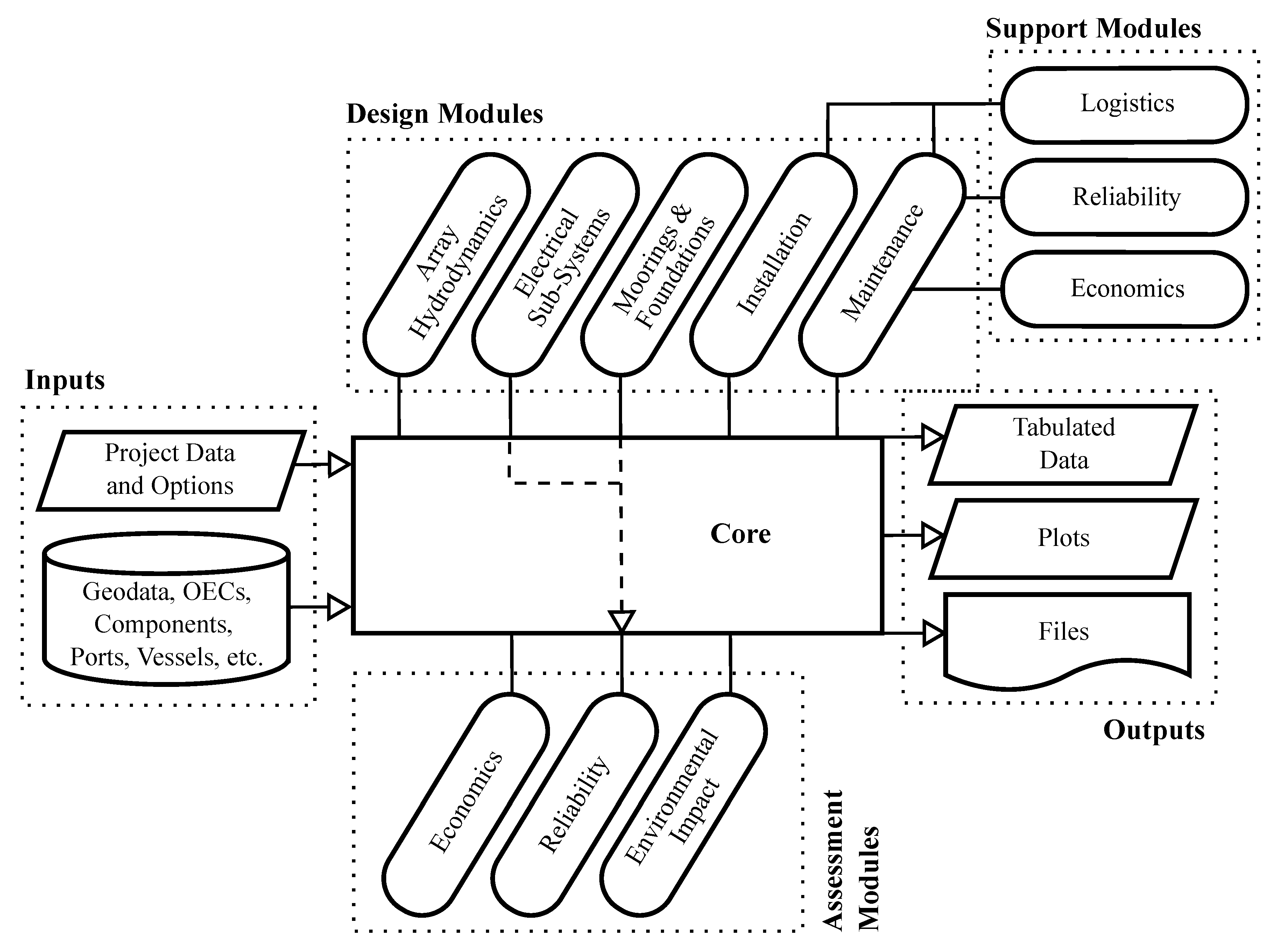
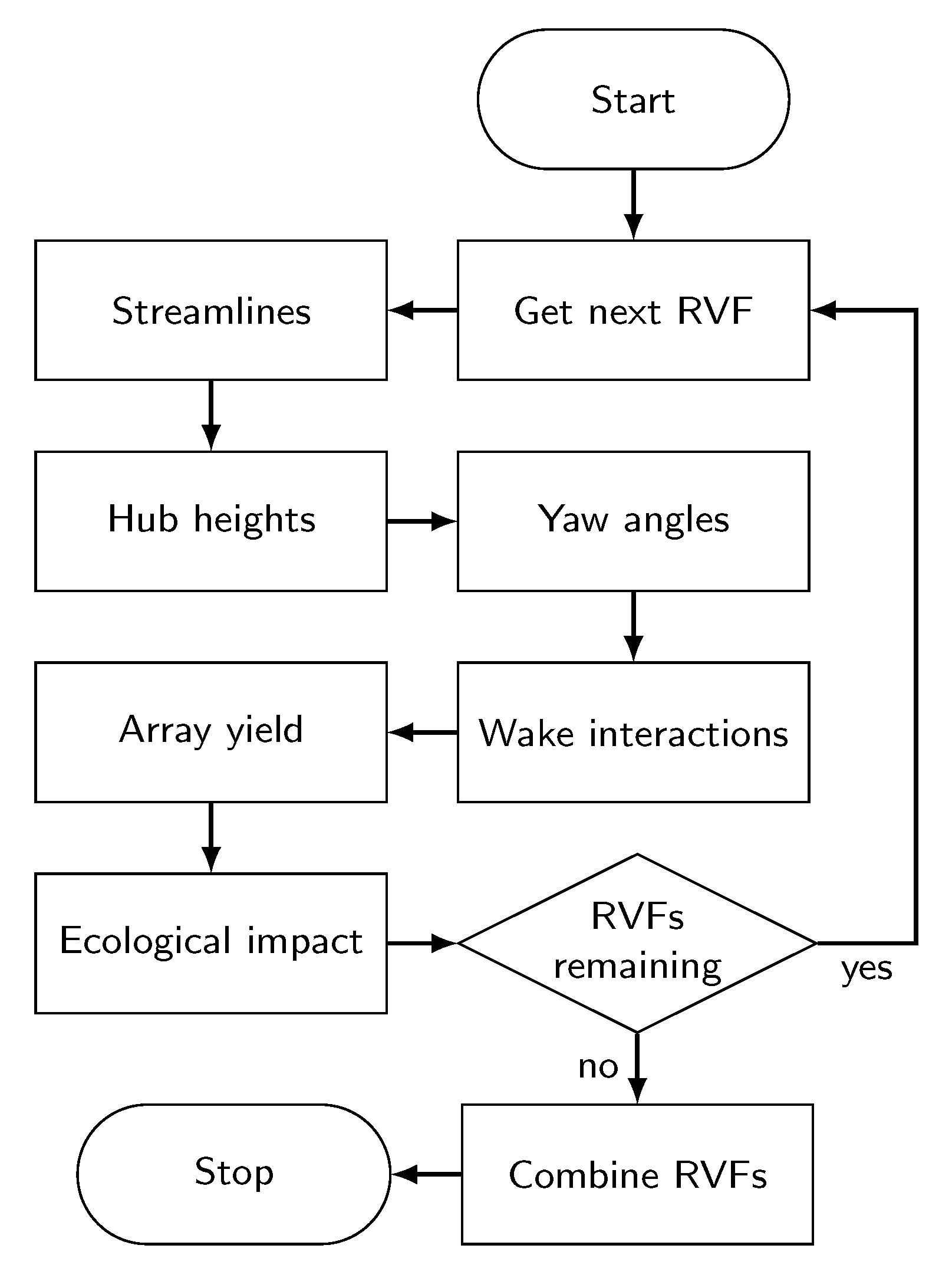
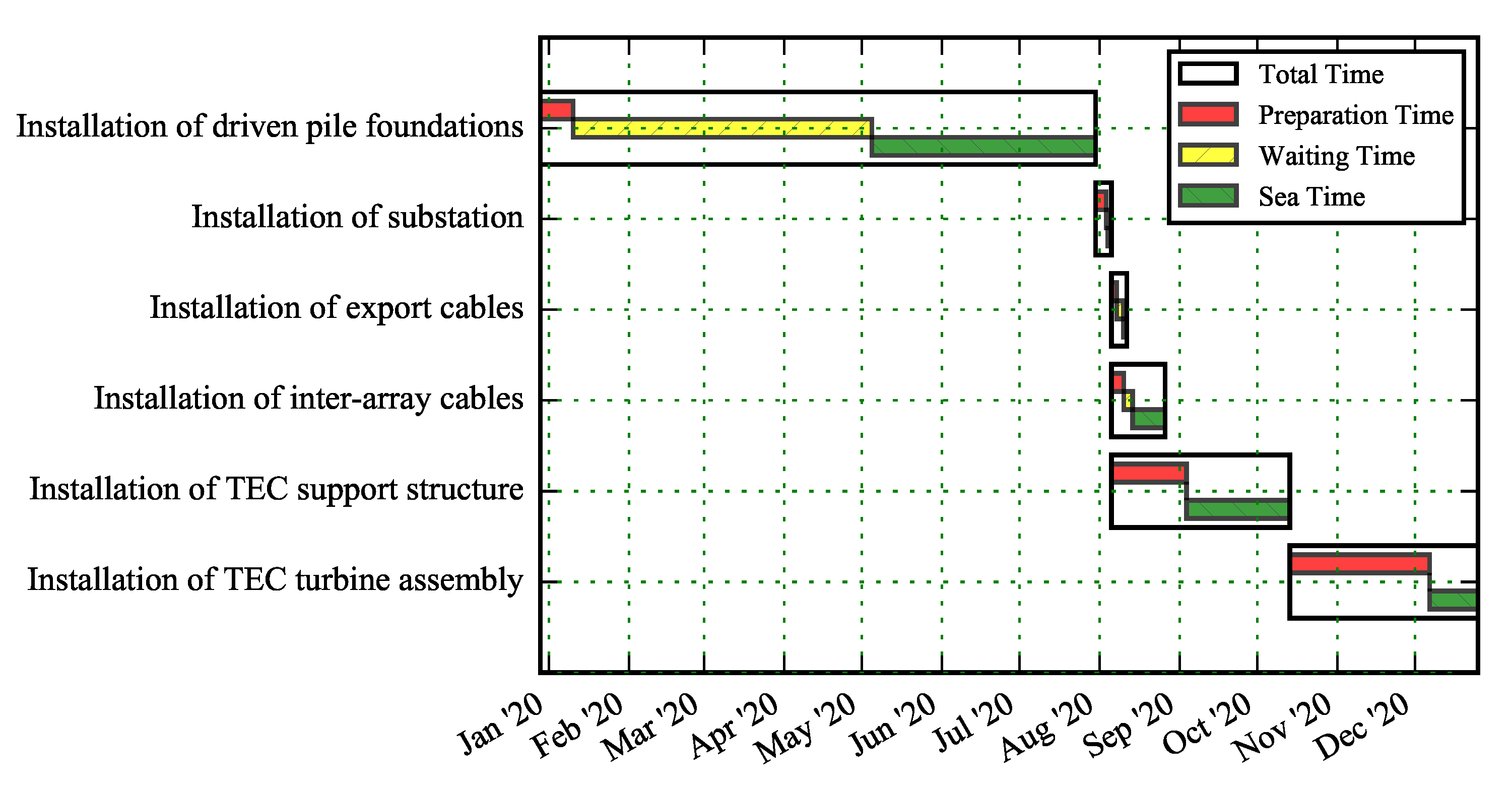
Figure 2 shows all the stages of the algorithm used in DTOcean, which will be discussed in the following subsections. Each stage is repeated for a number of representative velocity fields (RVFs), with each having an associated probability of occurrence. The selection of RVFs and calculation of the probabilities is described in 
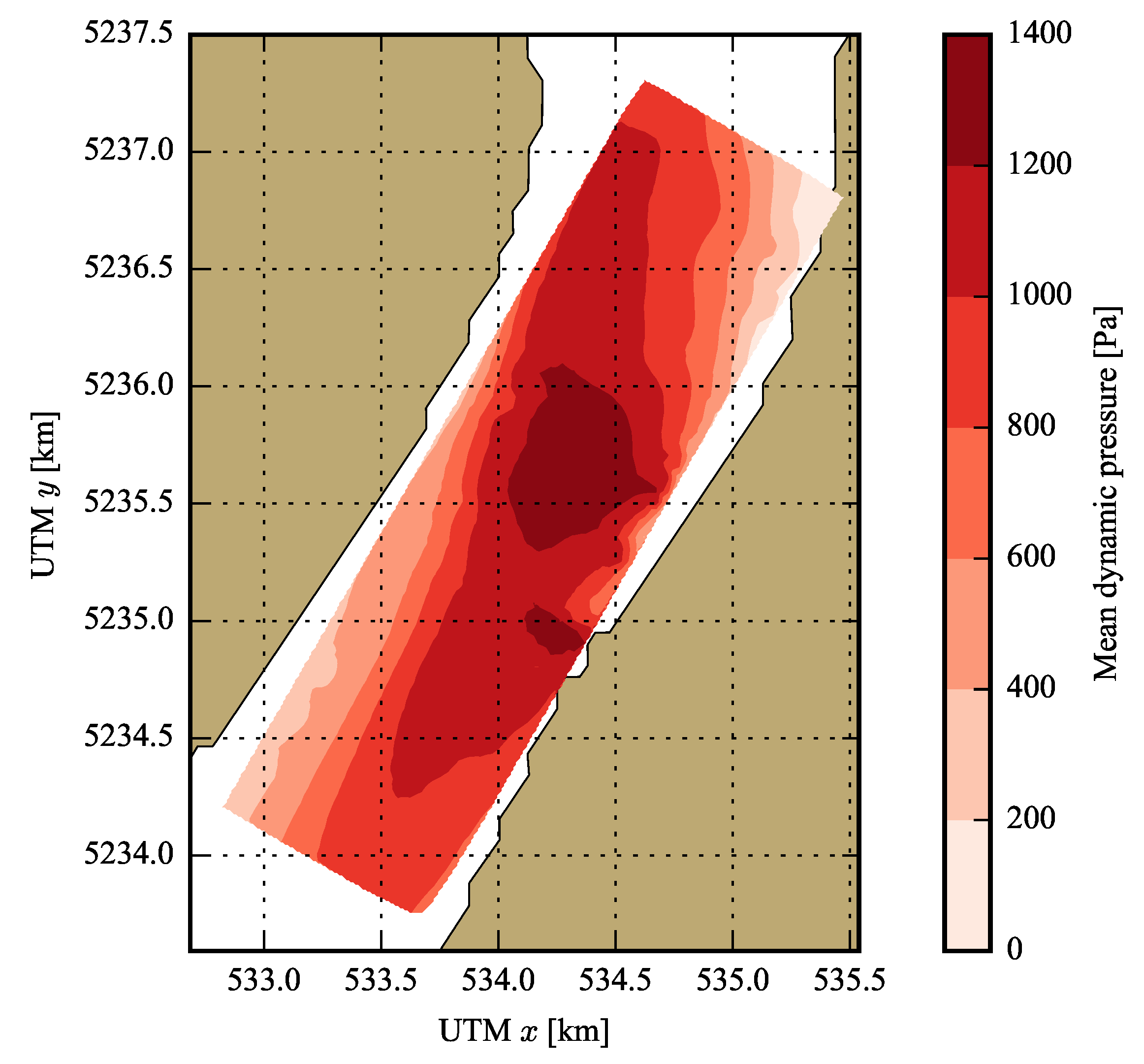
Appendix A. DTOcean uses a regular two-dimensional computational grid to store field data, as shown in 
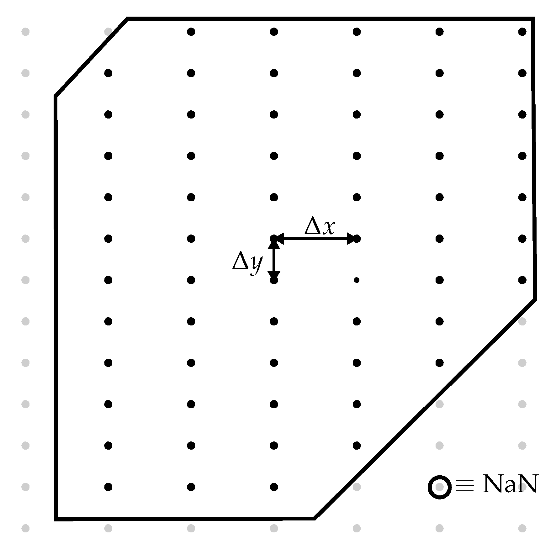
Figure 3, which contains bathymetric data, depth averaged tidal velocities and turbulence intensities. Where data are required at positions which do not intersect with a node of the computation grid (such as the location of TECs), values are interpolated linearly.

2.2.1. Streamlines

In order to apply a wake deficit along the streamlines emanating from each TEC rotor, the streamlines must first be calculated. It is assumed that the user or optimising algorithm has provided a set of TEC rotor locations p i for i = 1 , , n r rotors (for twin rotor systems n r is double the number of TECs). The flow field for each RVF is considered to be steady, and, thus, the streamlines can be determined by solving
d r d s = u ( r ) r ( 0 ) = p ,
where r is the position of a streamline parametrised by length s, u is the velocity at r and r ( 0 ) is the start of the streamline, which is equal to the position of the rotor of interest. Equation (2) is solved numerically using Euler’s method. To limit the error from the application of Euler’s method, the vorticity in the flow field is restricted by setting an upper limit.

2.2.2. Hub Height Adjustment

In the next stage of the calculation, the values of velocity and turbulence intensity within the 2D flow field are adjusted to account for the vertical position of the TEC rotors within the water column. The vertical profile of a tidally driven channel is complex and variable, both in terms of velocity and turbulence [29]. Accurately modelling such dynamic processes is extremely computationally expensive, thus, at the cost of some accuracy in velocity values and wake prediction, reduced order assumptions are used. As in [30], the velocity magnitude at height z above the sea bed, U ( z ) , can be estimated using a power law expression such as
U ( z ) = z β h 1 / α U ¯ ,
where U ¯ is the depth averaged velocity. β , known as the bed roughness coefficient, and α are calibrated to best represent the underlying physics. DTOcean’s original method for predicting β , given in [28], significantly underestimated its value, thus fixed values of β = 0.4 and α = 7 , as suggested in [31], were adopted for the present study.
As the TEC rotor operates over a range of depths, the difference in velocities between the top and bottom of the rotor is taken. Equation (3) can be written
U ( z ) = w U ¯ where w = z β h 1 / α .
Subsequently, the velocity over the rotor, U r is defined
U r = w r U ¯
where
w r = w top + w bottom 2
and w top and w bottom are the values of w for the vertical limits of the rotor. Note that this approximation improves upon methods that do not consider variation of velocity in the water column, but does not attempt the power weighted approach (“method of bins”) prescribed in [32]. Nonetheless, at the scale of problem investigated here, using the power law given by Equation (3), the errors in power production will be slightly under-estimated in comparison, which is deemed acceptable for a study of this nature. As with [32], the variation of velocity across the horizontal plane of the rotor is not considered in the calculation of U r .
To adjust the given turbulence intensity for the depth of the rotor consider that, under the assumption of homogeneous isotropic turbulence, the turbulence intensity, I, is given by
I = 1 U ( z ) 2 k 3 1 / 2 ,
where k is the turbulence kinetic energy. If k is also assumed to be uniform throughout the water column, it can be shown that
I r = I 0 w r ,
where I r is the turbulence intensity over the TEC rotor and I 0 is the turbulence intensity associated with the depth averaged velocity.

2.2.3. Rotor Yaw Angle

The next stage of the computation is the calculation of the angle between the rotor axis and the incident current, known as the ‘yaw angle’. This quantity is used both in the yield calculation and as part of the wake model. The TECs simulated as part of this study may not yaw, but do operate bi-directionally. In this case, the absolute yaw angle between the current and the rotor, ψ r , is given by
ψ r = min ψ u ψ 0 + π π ψ u ψ 0 π ,
where ψ u is the coincident angle of the current (looking upstream) and ψ 0 is the neutral orientation of the rotor (facing upstream). The operation between angle brackets is defined as
θ θ ( mod 2 π ) ,
where θ represents some arbitrary angle.
Each TEC simulated within DTOcean shares the same ψ 0 . If not set specifically by the user, the value is calculated from the most probable RVF in the input data. Let
u ¯ + = 1 n p i n p u i + and v ¯ + = 1 n p i n p v i + ,
where u ¯ + and v ¯ + are the mean velocity components of the most probable RVF, u i + and v i + are the velocity components of each point within the domain of the most probable RVF and n p is the number of points within the domain. Subsequently, ψ 0 = a t a n 2 ( v ¯ + , u ¯ + ) .

2.2.4. Wake Interactions

The next, and most complex, step in the energy extraction calculation is determining the velocities coincident with the TEC rotors subject to interactions with the wakes of other TECs. The approach taken in DTOcean to solve this problem follows a similar approach to the classic ‘Jensen’ model [
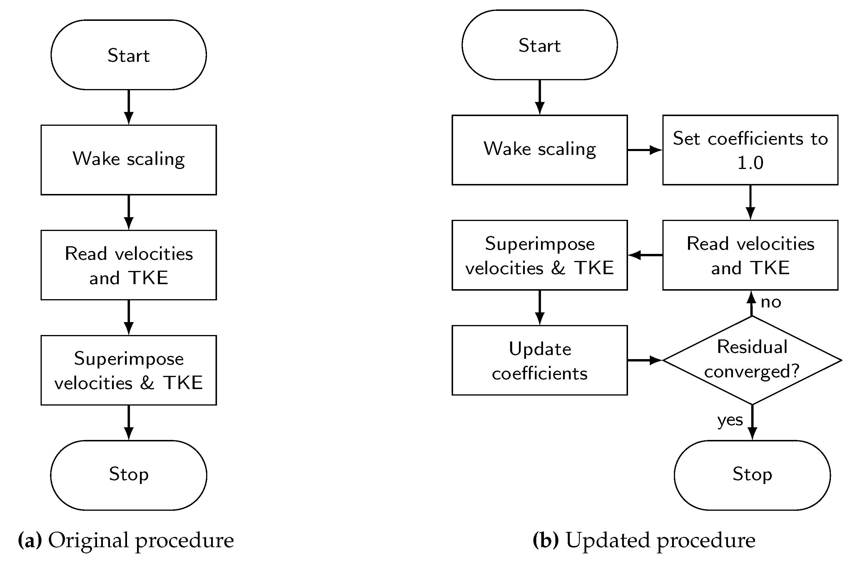
11], where superposition of parametrically defined wakes is used to determine the velocity deficits for arrays of wind turbines. Where Jensen used an analytical model to determine the induction factor (as defined in momentum theory), which is then used to determine the velocity of the wake, the approach in DTOcean is to directly access the velocities and turbulence kinetic energies within the wake of each TEC rotor using a database of normalised CFD simulations. In a further improvement to the Jensen model, the TEC wakes are assumed to develop along the streamlines emanating from each TEC rotor, rather than along the perpendicular to the rotor plane. Additionally, scaling of the modelled wakes can be used to account for blockage and rotor yaw angle. This process is illustrated in Figure 4a. Note that the process has been improved from that used in the original DTOcean software, as will be discussed further below.
As detailed in [28] (Section 3.3.3.4), a database of 2-dimensional CFD simulations (calculated using OpenFOAM [33]) was developed for use with DTOcean’s hydrodynamics module. The length scales (in the x and y planes) of the simulations are normalised by the rotor diameter, while the velocity scale is normalised by the local velocity upstream of the TEC. Subsequently, the remaining parameters affecting the development of the TEC wakes are the rotor’s thrust coefficient, C T , and the turbulence intensity of the incoming flow. The output field values are the scaling factor of the input velocity and the turbulence kinetic energy.
Beyond scaling the CFD simulations by the diameter of the TEC rotor being simulated, additional scaling can be undertaken to account for the effects of blockage and rotor yaw angle, as developed in [28]. Through numerical investigation, using the CFD TEC model (see [28]), it was determined that the x-axis of the CFD simulations should be scaled by a factor of 0.489 B 2 1.472 B + 1.0 , where B is the blockage ratio for the flow being investigated. DTOcean determines B through a combination of a user defined factor, B user , over the range [ 0 , 1 ] , and an additional factor determined as follows.
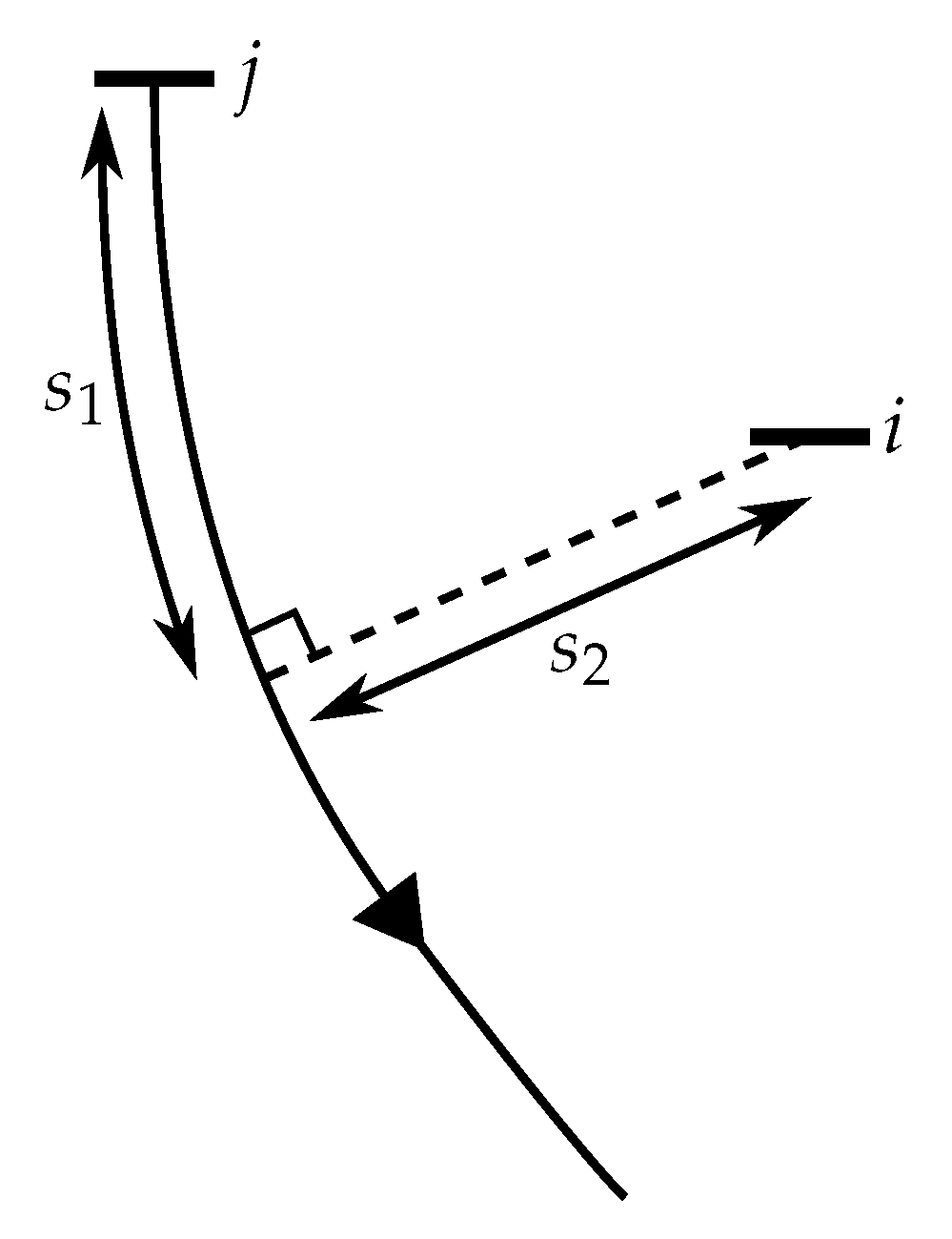
The distance of each TEC rotor relative to the streamlines of the other rotors (denoted X i j ) is calculated as shown in Figure 5. Subsequently, the first row of TECs ( i = 1 , , n 1 ) can be determined (i.e., those TEC rotors with no perpendicular interceptor with the streamlines of other rotors). Next, the area of a vertical transect across the deployment area coincident to the first row of TECs, A, is calculated. Finally, the blockage over the transect, B T , and the final blockage ratio, B, are given by
B T = i n 1 π D 2 cos ( ψ r ( i ) ) 4 A ,
B = B user B T ,
where D is the TEC rotor diameter and ψ r ( i ) is the yaw angle of rotor i. To account for the yaw angle of the rotor, the y-axis of the CFD simulations is also scaled, using a factor of cos ( ψ r ) .
The next stage is to update the velocity and turbulence intensity incident to each TEC rotor (subscript r is dropped), i.e.,
U i m = C U ( i ) U i 0
I i m = C I ( i ) I i 0
where U i and I i are the velocity magnitude and turbulence intensity for rotor i. The superscript 0 refers to the undisturbed state of the flow, while superscript m refers to the modified flow in the presence of the TECs. C U ( i ) and C I ( i ) are coefficients of the undisturbed velocity and turbulence intensity, for each rotor i, that are to be determined. By using Equation (4), Equation (7) can alternatively be written in terms of the turbulence kinetic energy and U i m as follows
I i m = 1 U i m 2 3 C k ( i ) k i 0 1 / 2
where k i is the turbulence kinetic energy at rotor i and C k ( i ) is the coefficient to be determined.
Reading from the database of CFD simulations can be described by the function
( C U ( i j ) , k i j ) = f ( B , D , ψ r ( j ) , X i j , C T ( U j ) , I j )
where the subscript i j refers to the value of the parameter at the position of rotor i subject to the influence of rotor j. Here, X i j maps the CFD solution onto the streamline emanating from rotor j and where X i j does not exist (such as for TECs in the first row), C U ( i j ) is set to unity and k i j = k j .
Once all coefficients C U ( i j ) and C k ( i j ) are known, they are superimposed. Several engineering approaches, as detailed in [34], exist to superimpose the velocity deficits predicted by Jensen style analytical wake models. In the original DTOcean code the ‘quadratic summation’ or ‘residual sum of squares’ (RSS) approach was used to superimpose the velocities, while the wake with maximum turbulence kinetic energy was used to directly calculate I i m (using Equation (4)). It was discovered in this work, however, that the function f can return a value greater than one, which exceeds the valid range of values for use in RSS approaches. Because of this, the current work uses the basic ‘dominating wake’ approach, where the wake with the greatest velocity deficit is chosen, i.e.
C U ( i ) min j C U ( i j ) .
Additionally, rather than use an alternative method to superimpose the turbulence kinetic energy, the value for the same dominant wake is used. If
γ = arg min j C U ( i j ) ,
then
C k ( i ) = k i γ k γ .
As seen in Figure 4a, at this stage the unmodified DTOcean code would calculate U i m and I i m and move onto the next stage of the energy extraction calculation. In the Jensen model, the values of U i m would be calculated for each row of downstream rotors in an iterative manner, to capture the compound affect of the wakes. Due to the non-uniform flow fields in tidal current energy simulations, identifying which TECs lie upstream of others is not straightforward, so the present work proposes to iterate all of the coefficients until convergence. Rewriting Equations (6) and (8) as
U i l = C U ( i ) l U i 0 , I i l = 1 U i m 2 3 C k ( i ) l k i 0 1 / 2 ,
where the superscript l represents the index of the iteration step, and combining Equations (9)–(12) as a single function
( C U ( i ) l + 1 , C k ( i ) l + 1 ) = g ( C T ( U j l ) , I j l ) ,
presents the problem in an iterative form. If C U and C k represent the coefficients for all n r rotors then let C U = C k = 1 for l = 0 and define the residual of the coefficient of velocity to be ϵ = C U l + 1 C U l . Finally, the iterations are considered converged if ϵ is less than a chosen value ( 1 × 10 4 was used herein). The complete process is illustrated in Figure 4b.
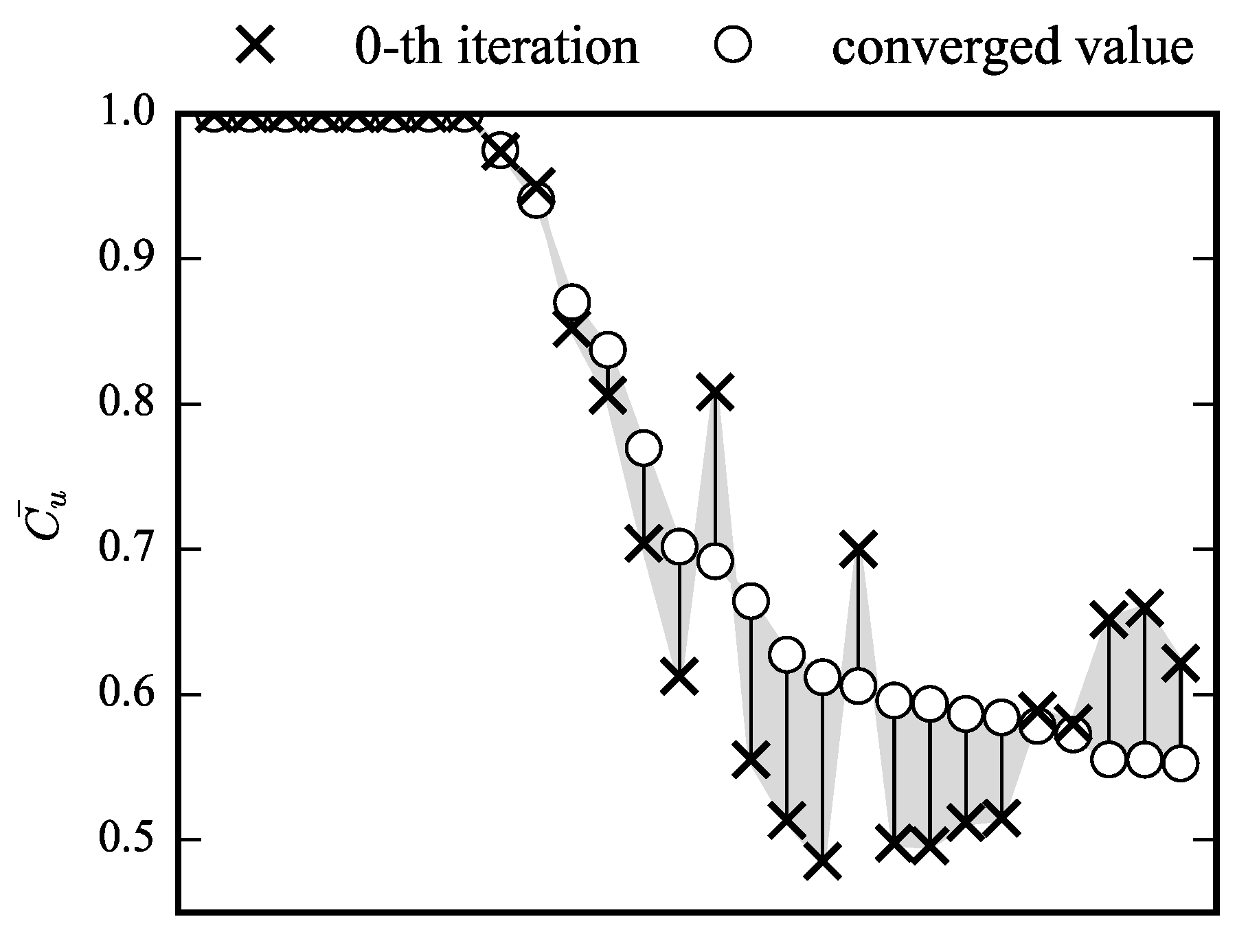
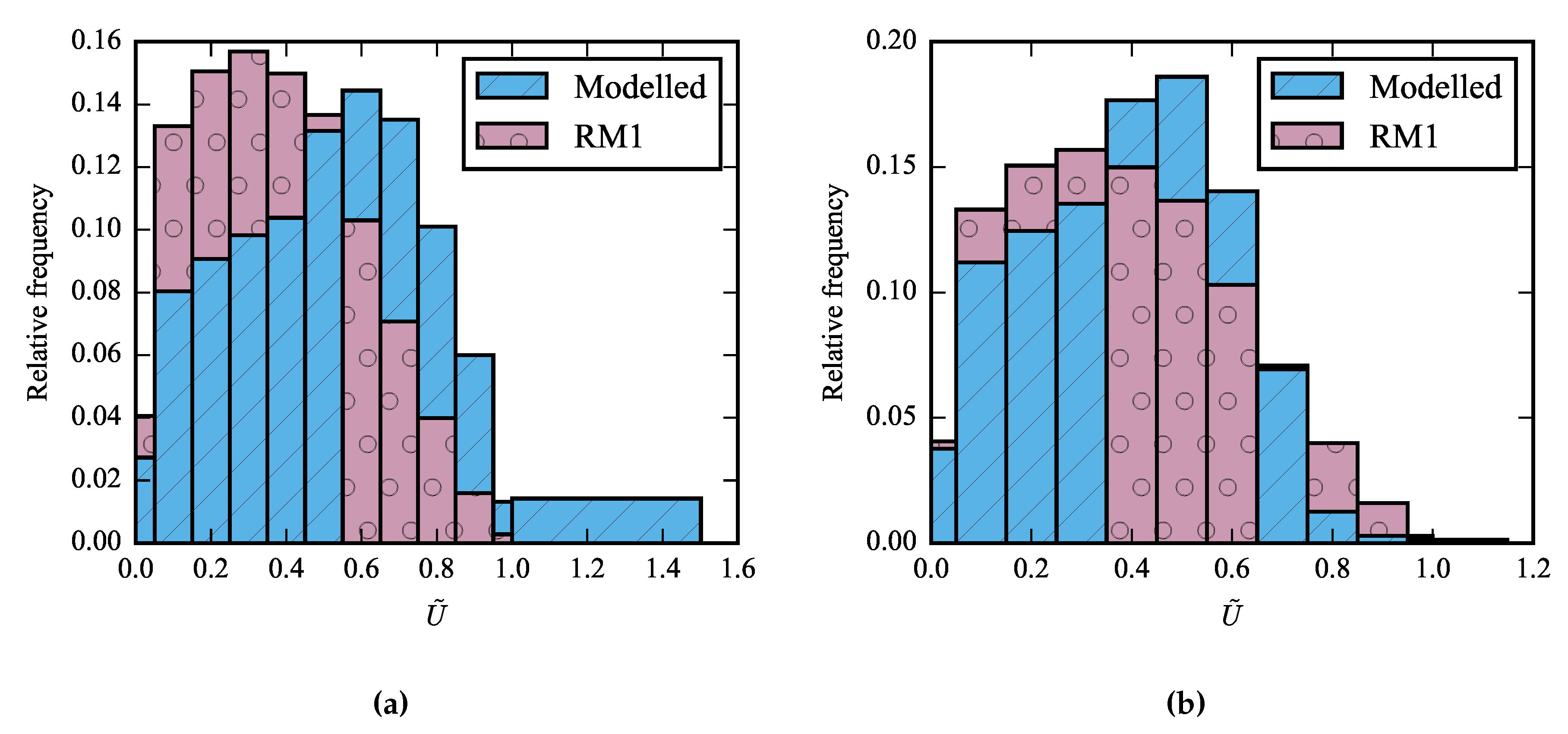
The value of using the proposed iterative solution over the original method in DTOcean is made clear by Figure 6. It can be seen that the mean value of C U for the initial iteration (analogous to the original DTOcean method) can both over- and under-estimate the converged value, and that the error can be significant across a range of values of C U .

2.2.5. Array Yield

For calculating the array yield for a particular velocity field, the power generated by the TEC rotor, accounting for the yaw angle, is given by [35] as
P i = π 8 ρ D 2 cos ( ψ r ( i ) ) C P ( U i ) U i 3
where C P is the coefficient of power for the TEC rotor, which varies by the velocity magnitude, U. For bi-directional rotors, the final power extracted from the TEC is also dependent on the rated power of the rotor generator, P rated , and the cut-in and cut-out velocities of the rotor, U in and U out . These rules are encapsulated as follows:
P i = P i U in U i U out P i P rated P rated U in U i U out P i > P rated 0 U i < U in U i > U out .

2.2.6. Combination of Velocity Fields

The final stage in the calculation of the energy extraction is to combine the power outputs from the TECs with the probability of occurrence of each RVF, to yield the MMAEP. Let P ( ω ) ( ω = 1 , , n s where n s is the total number of RVFs) represent the probability of each RVF, then
MMAEP i = 8760 × ω n s P i ( ω ) P ( ω ) , MMAEP = i n r MMAEP i ,
where P i ( ω ) is the power production of rotor i for velocity field ω , while MMAEP i and MMAEP are for rotor i and the array, respectively. MMAEP contributes to the denominator of Equation (1) as a product of the electrical losses and the percentage of generation lost to maintenance downtime, in each year of operation.

3. Case Study

This section will develop a case study to examine the effectiveness of the DTOcean software for techno-economic modelling of TEC arrays using the ‘Reference Model 1: Dual-Rotor Axial-Flow Tidal Turbine’ (RM1) reference model developed in [22]. This semi-analytical reference model considered a theoretical array of seabed-fixed tidal current energy converters which, although not a real deployment, provides sufficient detail to develop and test an effective DTOcean model.

3.1. Geography and Geology

The reference model considered TEC array deployment in the energetic tidal channel of the Tacoma Narrows, located on the west coast of the United States of America near Tacoma, Washington. Maximum current velocities in the Narrows were measured at just over 3 m s−1. The deployment area chosen was the area with the highest power density as reported in [21]. The location of the reference model relative to nearby infrastructure and population centres is shown in Figure 7.
The deep-water Port of Everett was identified to support installation, operation, and maintenance of the array, and was added to the DTOcean database of ports. It is assumed that the reference model’s TECs are manufactured locally and that various vessel assets can be acquired from within the US or beyond. No specific grid connection infrastructure is present near the reference model’s deployment site, and the banks of the Tacoma Narrows are highly populous, with numerous parks and preservation areas. A potential connection site, identified in this study, is the disused Western Slopes water treatment plant, situated just south of the eastern landing of the Tacoma Narrows bridge, as shown in Figure 8. This infrastructure could be re-purposed to support the array deployment, although horizontal directional drilling would still be required to land the export cable, as rail transit assets lie between the water treatment plant and the Narrows’ shoreline. The proposed export cable landing point is also shown in Figure 8.
Array scales of 10 and 50 TECs will be compared, with deployment areas defined to allow the spacing requirements specified in [22] (400 m longitudinal and 115 m lateral), as shown in Figure 8. A 100 TEC simulation was also included in [22], but, at the given spacing between TECs, this array would need to curve at the northern end of the channel, which is beyond the present capabilities of DTOcean (as every TEC must share a single orientation). The defined deployment areas occupy roughly 80% of the width and depth of the channel, thus the user defined blockage factor, B user , (see Equation(5)) is set to 0.8 . Bathymetric data for the deployment areas were acquired from public sources (NOAA and USGS websites) and are shown in Figure 8. Although sediment data was not reported in [22], various historic surveys were compiled in [19] which indicate that the strata are a mixture of dense sand, gravel and cobble, with patches of hardpan. As a detailed map of the different layers of stratum is presently unavailable, a single layer of ‘gravel cobble’ type was chosen for the DTOcean model.
A time series of current velocity values is required for each grid point within the deployment areas. A hydrodynamic model of south Puget Sound, created using the Delft3D Flexible Mesh Suite [36], was used to generate thirteen days of data. It was found that the boundary-conditions used in [21] resulted in a much less energetic channel than the values used to calculate the power outputs in the reference model, shown in [22], Figure 3-5. To more accurately represent the flow conditions used in the reference model, the boundary conditions were adjusted to a sole M2 astronomical component with an amplitude of 2 m. Figure 9a compares the relative frequency histogram from [22], Figure 3-5 with all points from within the updated Delft3D simulation. It can be seen that, overall, the Delft3D simulation has higher peak and median velocities than the reference model data. To gather insight on the effect of using a modelled velocity field, without biasing the results due to the higher kinetic energy content, a scaling factor was applied to the modelled velocities to equalise the mean dynamic pressure (MDP) of the two velocity histograms, given by
q = 1 2 ρ i V c ( i ) 2 F i ,
where V c ( i ) is the mean velocity and F i is the relative frequency of bin i, respectively. The scaling factor is then given by q RM 1 / q D 3 D , where q RM 1 and q D 3 D are the MDP calculated from the relative frequency histograms for the reference model and Delft3D velocities, respectively. The comparison between the original and scaled velocities is shown in Figure 9b. Use of the scaled velocities will improve the likelihood that the DTOcean simulations will match the energy production predicted in [22], yet the energy outputs may still differ, due to the velocities distributions being dissimilar (e.g., those in Figure 9b) and spatial variation in the channel (illustrated by the distribution of mean dynamic pressure shown in Figure 10). Also, as DTOcean requires depth averaged velocity values as inputs, the correction of velocity due to the TEC’s depth in the DTOcean model may result in higher values than the mid-stream values reported in [22].
For each velocity value in the DTOcean input, the associated turbulence intensity must also be given; however, as the Delft3D model was run in 2D mode (to ensure sensible simulation time), turbulent quantities were not calculated. Therefore, a constant of 10% was used throughout (as measured by [37]). Finally, the bathymetric, velocity, and turbulence data were interpolated onto a 10 m computational grid.
Extreme values must be supplied for the design of subsea and surface-piercing structures. Following [22], the design wind velocity was set to 40 m s−1 while the limit of TEC survival was defined by the ‘shock’ failure mode where the maximum thrust coefficient is combined with 2.85 m s−1 currents. Additionally, long term, representative environmental values are required for calculating the logistical operations. Five years of continuous, concurrent data were available in the public domain, with wind data collected from the anemometer located on the NDBC C-MAN ‘WPOW1’ station in West Point, Washington and current data originating from predictions for the NOAA ‘PUG1527’ sensor station, located within the Narrows. It has been shown in [38] that the occurrence of waves which are large enough to have any impact on the design or operation of the arrays is extremely unlikely. Given that the impact of waves was also not considered in [22] and that no routine measurements are taken within the Tacoma Narrows, all wave values used by DTOcean were set to zero.

3.2. Tidal Energy Converter

The TEC studied is known as the ‘RM1 device’, defined in [22] (Chapter 3). The TEC design emulates that of the SeaGen converter [39] and generates power through the transfer of kinetic energy from the tidal current to the rotational energy of the generators of two rotors connected by a crossbeam, as seen in Figure 11.
The crossbeam is 28 m in length and mounted atop a monopile of 45 m height and 3.5 m diameter (where 15 m of the monopile’s height is below the seabed). The TEC rotors are 20 m in diameter and are a two-blade design which may operate bidirectionally with the current. The rotor nacelles are 8.3 m in length and 2.4 m in diameter and contain the power converters (to electrical energy, in this case).
The RM1 device design incorporates the foundation into its tower, with the bottom 15 m being driven into the seabed. DTOcean is not capable of assessing the viability of such an integrated foundation, so a proxy model was sought. By considering the tower to be 30 m tall rather than 45 m and allowing the module to design a pile foundation for the tower, the design choices of the tower can be compared. The idealised dimensions and other characteristics required to design the foundations are given in Table 3, as derived from [22].
The RM1 device has a rated power of 1.1 MW with two rotors per TEC resulting in 550 kW per rotor. The power take-off was designed for a cut-in velocity of 0.5 m s−1 and a cut-out velocity of 3 m s−1. The power coefficients of the rotors were reverse engineered from the power curve shown in [22], Figure 3-7. No thrust data was available, so momentum theory was used to estimate the thrust coefficients, by numerically calculating the axial induction factors corresponding to the power coefficients, assuming the axial induction factor is restricted to the range [ 0 , 1 / 3 ] . The thrust coefficients follows accordingly. The power and thrust coefficient curves are shown in Figure 12.

3.3. Project Design and Economics

A staggered grid layout, which allows the longitudinal and lateral spacing between TECs to be varied, was chosen for optimization of the TEC positions with respect to MMEAP. The minimum distance between TECs was set to 90 m ( 4.5 D ) in the lateral and 375 m ( 18.75 D ) in the longitudinal directions, in order to reproduce the idealised spacing suggested in [22] of 115 m ( 5.75 D ) lateral and 400 m ( 20 D ) longitudinal, allowing some slack. Padding of 20 m, twice the grid discretisation, was placed between deployment area boundary and the TECs to ensure successful calculation of cable connections and seabed gradients. The gridded tidal current velocity data were processed into twenty RVFs (using the procedure described in Appendix A), which provides comparative accuracy to [22] and reasonable computational cost.
The installation method for the TECs’ foundation piles is optimised in DTOcean by testing multiple feasible installation techniques. In [22] a pile driver is specified and it states that three piles can be installed per day ([22], Figure 3–19). This translates to a penetration rate of 2 m h−1 and, to ensure consistency, the penetration rate for gravel cobble stratum used in the DTOcean simulations was set to 2 m h−1 (from 5 m h−1). All other techniques available for installation of piles were disabled.
To model the rotor assembly design, which allows installation and retrieval at any point in the tidal cycle, all related installation and maintenance limit conditions were set to a maximum current speed of 3 m s−1. In [22] a calendar-based strategy was used to maintain the TECs over the lifetime of the array. It suggests the RM1 device would require two maintenance actions (to service the rotor and power take-off (PTO)) annually per TEC while there would be no failures to the electrical network (due to the burial of cables). As detailed in [25], DTOcean can simulate a calendar interval-based maintenance model for the TEC sub-systems, based on the failure rate, λ . Defining the mean time to failure (MTTF) as MTTF = λ 1 , and assuming that sub-systems exhibit perfect reliability prior to their given MTTF, the probability of failure of a sub-system before time t is:
P f ( T t ) = 0 t MTTF 1 exp λ t t > MTTF
where T is the time of failure.
A failure rate of 57.1 failures per million, which equates to one failure every two years, was applied to both the rotor and PTO, separately, and the maintenance interval is set to match. As there are two nacelles per TEC (housing two sub-systems each), the TECs will undergo maintenance twice annually, on average. Following [22], the support structure is given a design life of 40 years and the structure, foundations, and electrical network are not maintained, being subject to random failure. These balance-of-plant systems may have an impact when comparing the operational expenditure (OPEX) of DTOcean to the reference model. For instance, the electrical network will not exhibit perfect reliability in DTOcean, as the failure rate of cables is invariant with the method of installation, while the reference model assumes no failures will occur because the cables are buried. Note that the DTOcean maintenance module does not consider the partial failure of a TEC (i.e., loss of power from one of the two rotors) and any sub-system failure is considered to cause total loss of generation.
All failure modes for the RM1 device defined in [22] require maintenance to be undertaken at port (the entire cross-beam and nacelle assembly is removed), which is not explicitly modelled by DTOcean. To provide a proxy, the failure modes of the TEC were assumed to require on-site maintenance (with spares costing 10% of the total sub-system cost) with four maintenance actions allowed per journey (representing service of the rotor and PTO on both nacelles). Additionally, [22] assumes a bespoke, dedicated maintenance vessel is purchased to carry out all TEC recovery operations. DTOcean is currently not able to directly simulate this choice as it does not allow a ‘preferred’ vessel to be chosen from the database of vessels, nor does it include purchase costs for vessels. To simulate the operating costs of the purchased vessel, without specifically entering the TEC specifications into DTOcean, the day rates for all used vessels were set to zero (crew costs were still included). The vessel purchase cost, fixed to the value of the vessel described in [22], was then included as an external capital expenditure (CAPEX) cost.
Following [22], port costs were included as 5% of the total installation expenditure and a 25% contingency cost (of the final installation costs) was added. A further cost, which cannot be incorporated directly into the results of the installation module, is incurred by the use of a sound barrier system, to reduce the underwater noise created by the piling activities. This additional cost was added to the external CAPEX costs, summarised in Table 4. Table 5 summarises the additional annual contributions, from insurance and environmental monitoring, to be added to the OPEX costs. The total external CAPEX and OPEX is converted to Euros, with a conversion factor of 0.85, for entry into DTOcean. The commencement of the array installation is scheduled for the arbitrary date of 1st January 2020. The project duration is set to 20 years and the discount rate used in the LCOE calculations is set to 0.113, which includes the discount rate, tax and inflation contributions which are included in the LCOE calculations within [22]. Following [25], thirty samples of OPEX and AEP are used to determine the variability present in the predicted LCOE values.

4. Results

The array layouts for the 10 and 50 TEC arrays are presented in Figure 13 and Figure 14, respectively. The MMAEP for the two scenarios are given in Table 6 and Table 7, with comparison to the values used in [22]. For 10 TECs, the optimiser selected spacing of 125 m (6.25D) in the lateral and 398 m (19.9D) in the longitudinal directions, while for 50 TECs the distances were 101 m (5.05D) in the lateral and 386 m (19.3D) in the longitudinal. To allow enough TECs to be deployed, depth limits of 45–67.5 m were required, which exceeds the 50–60 m limits given in [22].
DTOcean was incapable of designing an electrical network with branches connected to a shared trunk cable, as proposed in [22], instead designing branches emanating from a single substation, used to supply the export cable. This network layout results in more TECs per branch than the ‘row-by-row’ network, which has a negative impact on efficiency of the network. To maintain a reasonable level of network efficiency, network voltage ratings were calibrated to 11 kV for the TEC (which also determines the rating of the inter-array cables) and 33 kV for the export cable. The electrical network efficiency and capacity factor for the two scenarios are given in Table 6 and Table 7, with comparison to the values used in [22]. No electrical losses were considered in [22], but DTOcean predicts 5.8% energy loss for the 50 TEC array. Additionally, due to the steep seabed gradients within the channel, (vertical) cable installation angles of 11 . 25 are necessary, which is steeper than the typical 10 limit for subsea cable installation [40].
The TEC foundation safety factors were calibrated to a value of 3.6 to achieve a diameter and depth of pile similar to the RM1 device tower, which is greater than the safety factor of 1.65 given for the combined tower and foundation design in [22]. DTOcean specified a pile diameter of 3 m at an installation depth of 15 m. The substation also required a pile foundation which was designed with a 5 m diameter tube pile requiring an installation depth of 18 m.
The Gantt chart for the 50 TEC scenario, incorporating the major installation phases, is shown in Figure 15. The inclusion of waiting time between slack tides and the delay in starting operations (to minimize waiting time) extends the total installation time to 13 months for 50 TECs. The mean annual maintenance operations, mean array availability, and mean lifetime energy production are given in Table 8. As can be seen, very few non-scheduled maintenance events occur, leading to very high plant availability, in general.
The levelised cost of energy for DTOcean, with comparison to the results of [22] (denoted ‘RM1’), are given in Table 9. The most likely value of the DTOcean results and the 95th percentile range are shown. The absolute error in most likely value is 0.0208 €/kWh for 10 TECs and 0.03 €/kWh for 50 TECs with relative errors of 6% and 17.3%, respectively. The absolute 95th percentile range is 0.0073 €/kWh for 10 TECs and 0.0148 €/kWh for 50. Table 10 and Table 11 compare the LCOE breakdown per cost category between [22] and the DTOcean simulation, using DTOcean’s most likely LCOE.

5. Discussion

The headline figures for LCOE, given in Table 9, indicate that the reproduction of the RM1 reference model in DTOcean performs reasonably well for 10 TECs, with increased absolute and relative error for 50 TECs. Economies of scale considered in the reference model, which are not modelled in DTOcean, play some part in this difference, but other modelling differences are also significant. Indeed, there are several design differences and deficiencies in both the DTOcean model and the reference model, some of which act to balance the predicted LCOE.
For both 10 and 50 TECs, the DTOcean simulations exceed the energy production predicted in [22], which is expected as the depth constraints on the TEC locations generally coincide with more energetic regions within the deployment area, and depth correction of the input velocities will also have an impact. This shows the limitations of using a single value to predict the output of all TECs placed within a complex domain, as applied by [22]. Neither the RM1 study nor DTOcean considers the potential impact on the resource from the existence of the arrays, which may further reduce power output and economic efficiency.
The complex bathymetry in the Narrows prohibits the perfectly regular rows expected by the reference model’s array layout, as seen in Figure 13 and Figure 14. Yet, it is clear that an electrical network which uses a single bus cable joining branch cables for each row, as proposed in [22], would be more practical than the central substation design, created by DTOcean. Such a design would allow shorter branches and less TECs per branch (although it is unknown if construction would be possible given the steep seabed gradients). Nonetheless, the drop in electrical efficiency caused by the substation-based layout brings the capacity factor of the 50 TEC array closer to that predicted in [22].
To match the TEC foundation design given in [22], higher safety factors were required than expected. This discrepancy may lie in the fact that DTOcean is only calculating the requirements for the foundation part of the integrated tower. Uncertainty regarding the characteristics of the bed sediment may also be a factor, as these are not reported in [22] and little detail is provided regarding the foundation design calculations. The large diameter pile for the substation is necessary as DTOcean only supports surface piecing substations, and so it must resist both the extreme currents and wind speeds. No such additional in-stream infrastructure is mentioned in the reference model, which is likely due to the short distances to shore, although, as discussed in Section 3, available real estate on the Tacoma Narrows shoreline is limited.
Another cause of difference in LCOE between the two models are the array installation calculations. In [22] there is no attempt to estimate the real time required for completing the installation, instead opting to add a 25% cost contingency to cover delays; however, adding extra cost alone is inadequate for capturing the effect of long installation times, as delay in energy production will have an impact on the final LCOE value for the array. DTOcean’s advanced operations and maintenance calculations were another potential source of discrepancy, but even though some faults were detected in the electrical network and TEC support structure, which are not considered in [22], these have limited impact, overall. This is because of the intrinsic high costs created by the twice annual maintenance routine specified in the reference model.
Ultimately, even though the DTOcean simulation produced more energy than predicted in [22], DTOcean over-predicts the LCOE at both scales of deployment. The variability in the LCOE is small (less than 0.02 €/kWh), with little change between scales, which is expected given the highly prescribed maintenance strategy used for the array and the lack of seasonal variation in the current velocities. It is somewhat challenging to analyse the differences between contributing cost factors, as several costs considered to be externalities in the DTOcean simulations are included within other cost categories for the reference model. This includes the vessel purchase which, although not explicitly stated, is presumably included in the ‘Infrastructure’ category of the reference model, which also includes the electrical network and therefore is compared with DTOcean’s electrical network in Table 10 and Table 11. Also, the sound barrier is included in the reference model’s installation costs, but added as an externality for the DTOcean model. Despite these caveats, it is credible that the additional costs in DTOcean primarily lead from foundation components costs (excluded from the reference model due to the integrated TEC design) and the increased cost of installation due to the need to wait for slack tides. Economies of scales are also applied to certain costs in [22], which are invariant with respect to deployment scale in DTOcean.

6. Conclusions

The capability of the DTOcean software to model the techno-economic performance of ahydrokinetic tidal energy converter (TEC) array has been verified through modelling and comparison of the levelised cost of energy (LCOE) of the RM1 reference model [22], a hypothetical TEC deployment within the Tacoma Narrows of Washington state, U.S.A.
Following an overview of the DTOcean software, the tidal hydrodynamics module of DTOcean’s original release was revisited and improved, including adding an iterative solver to the ‘Jensen’ model used to calculate the TEC wake interactions, as detailed in Section 2.2. Given the sensitivity of LCOE to the energy production of the TEC array, these improvements will increase the accuracy of DTOcean’s predictions with respect to the original method used in the software. The remaining software was unaltered from that applied in [25]. Subsequently, it was demonstrated that the DTOcean suite, including the improved tidal hydrodynamics solver, produced reasonable estimates to the LCOE values given in the reference model. For 10 TECs, DTOcean calculated a most likely LCOE (in Euro cents per kiloWatt hour) of 34.612 ¢/kWh to the reference 36.69 ¢/kWh, while for 50 TECs, DTOcean calculated 20.34 ¢/kWh compared to 17.34 ¢/kWh for the reference model.
There were several discrepancies between the designs which exposed weaknesses in the methodologies of both DTOcean and the reference model. In particular, the method used for energy estimation in the reference model failed to account for variation of the flow within the channel or within the water column. Also, important design information was absent, including the sea bed sediment in the channel and the foundation design calculations. DTOcean could not reproduce the electrical network design proposed in the reference model, adding a dedicated surface piercing substation (and foundation) as a collection point when a subsea bus was mandated. Also proxies for the integrated TEC foundation, maintenance vessel purchase, and repair at shore maintenance mode, had to be found. Comparison of the cost factors between DTOcean and the reference model was challenging as the contributors to the categories are not given in [22]. The most probable causes for the increased error in LCOE value between 10 and 50 TECs are economies of scale included in the reference model, which are not considered by DTOcean, and the impact of installation duration, which is not considered in the reference model.
At minimum, this study demonstrates that DTOcean can be useful to designers of TEC arrays, due to the systematic process it enforces and by capturing interactions between disparate data sources. For instance, the bed sediments were overlooked in the RM1 reference model, but sediment type can have a significant impact on the costs and time required for installation. In this way, the RM1 study was a useful comparison tool for DTOcean as it demonstrated areas where conventional analytical design can overlook important factors. Obviously, confidence in the predictive capability of DTOcean would be further improved by studies involving real arrays but, at time of writing, no such data is available in the public domain.
Beyond addressing the issues mentioned above, further work should consider arrays of single turbine TECs, whilst modelling TECs with individual orientations (all TECs must have the same orientation in DTOcean, at present) will allow for larger arrays to be simulated, such as the 100 TEC RM1 reference model array. At such scales, considering any potential reduction in resource from the existence of the array will also be vitally important.

Author Contributions

Individual contributions from authors are as follows: conceptualization, M.B.R.T., S.S.O. and J.D.R.; methodology, M.B.R.T.; software, M.B.R.T.; validation, M.B.R.T.; formal analysis, M.B.R.T.; investigation, M.B.R.T. and S.S.O.; data curation, M.B.R.T. and S.S.O.; writing–original draft preparation, M.B.R.T.; writing–review and editing, M.B.R.T., S.S.O. and J.D.R.; visualization, M.B.R.T.; funding acquisition, J.D.R.; All authors have read and agreed to the published version of the manuscript.

Funding

Sandia National Laboratories is a multimission laboratory managed and operated by National Technology & Engineering Solutions of Sandia, LLC, a wholly owned subsidiary of Honeywell International Inc., for the U.S. Department of Energy’s National Nuclear Security Administration under contract DE-NA0003525. This paper describes objective technical results and analysis. Any subjective views or opinions that might be expressed in the paper do not necessarily represent the views of the U.S. Department of Energy or the United States Government.

Acknowledgments

Special thanks are given to Lucy Cradden for her editorial contributions to this manuscript. The image of the RM1 device, in Figure 11, was adapted with the permission of Sandia National Laboratories.

Conflicts of Interest

The authors declare no conflict of interest. The funders had no role in the design of the study; in the collection, analyses, or interpretation of data; in the writing of the manuscript, or in the decision to publish the results.

Abbreviations

The following nomenclature and abbreviations are used in this manuscript:
Bblockage ratio
C k ( i ) coefficient of undisturbed turbulence kinetic energy for rotor i
C k ( i ) l coefficient of undisturbed turbulence kinetic energy for rotor i at iteration l
C T rotor thrust coefficient
C U coefficient of undisturbed hub velocity
C U ( i ) coefficient of undisturbed hub velocity for rotor i
C U ( i j ) coefficient of undisturbed hub velocity for rotor i subject to rotor j
C U ( i ) l coefficient of undisturbed hub velocity for rotor i at iteration l
DTEC rotor diameter
I i turbulence intensity for rotor i
I i 0 undisturbed turbulence intensity for rotor i
I i l modified turbulence intensity for rotor i at iteration l
I i m modified turbulence intensity for rotor i
P i constrained rotor power output for rotor i
P i unconstrained rotor power output for rotor i
U i hub velocity for rotor i
U i 0 undisturbed hub velocity for rotor i
U i l modified hub velocity for rotor i at iteration l
U i m modified hub velocity for rotor i
X i j distance from rotor i to streamlines of other rotors
k i turbulence kinetic energy for rotor i
k i j turbulence kinetic energy for rotor i subject to rotor j
k i 0 undisturbed turbulence kinetic energy for rotor i
n r number of TEC rotors
ψ 0 neutral orientation of rotor
ψ r absolute yaw angle between current and rotor
ψ r ( i ) absolute yaw angle between current and rotor for rotor i
ρ water density
AEPannual energy production
CAPEXcapital expenditure
LCOElevelised cost of energy
MMAEPmechanical mean annual energy production
OPEXoperational expenditure
PTOpower take-off
RVFrepresentative velocity field
TECtidal energy converter

Appendix A. Resource Characterisation

The DTOcean modules are designed to operate in a technology agnostic fashion. To achieve this, resource data is provided as a set of static hydrodynamic ‘states’, with an associated probability of occurrence. Whereas a sea state is commonly understood in the context of wave energy resources (i.e., the likelihood of occurrence of a particular range of wave height and period), tidal energy resources are not commonly classified in this manner. To ensure compatibility across DTOcean, a statistical representation of tidal current flows was devised, herein known as representative velocity fields (RVFs).
The user of DTOcean is required to provide a representative time series of depth averaged tidal velocities and turbulence intensity for each point of the computational grid (shown in Figure 3). Ideally, an hourly time series over a single tidal cycle should be provided, although in the case of very large domains, it may be necessary to reduce the number of time steps to avoid excessive memory usage. To establish a set of RVFs from the given time series, a single grid point from within the domain is selected, from which a time series of velocities is extracted. As an example of the process, 28 days of easterly and northerly (with respect to true North) velocity components, denoted u and v respectively, from the NOAA Cherry Point monitoring station was extracted, and resampled as hourly values, as shown in Figure A1. Note that the Cherry Point velocities are measured at the near sea surface, rather than depth averaged.
Figure A1. 28 days of near surface easterly and northerly (with respect to true North) velocities components. Measured at the NOAA Cherry Point monitoring station, in units of centimetres per second, and resampled to hourly values.
Jmse 08 00646 g0a1
The extracted time series is processed into a discrete bivariate probability density function (PDF). The velocity component with the greatest range is classified as the principal direction, v p , while the other is classified as the secondary, v s . Subsequently, the data is binned into a two dimensional histogram, described by
N = i = 1 K p j = 1 K s M i j
where N is the total number of observations, K p is the number of bins in the principle direction, K s is the number of bins in the secondary direction and M i j is a function that counts the number of observations within each bin. K p is chosen by the user and is equal to the desired number of RVFs. The range of each bin in the principal direction is
[ R i , R i + 1 ) i < K p i , R i + 1 ] i = K p
where R is the set of values dividing the bins.
In the secondary direction, the measured values are binned into fixed width bins chosen to encompass all of the available data, i.e.,
K s = max v s min v s h
where h is the bin width and the braces indicate the ceiling function. The bins are centred over v s and range of each bin in the secondary direction is given by
[ S i , S i + 1 ) i < K s i , S i + 1 ] i = K s
where S is the set of dividing values. The discrete PDF is then defined as
PDF i j = m i j N .
For the Cherry Point example, the resulting discrete PDF is shown in Figure A2a, using K p = 10 . The secondary bin width is set to h = 1 cm s−1, the default value used by DTOcean.
Figure A2. Probability density calculated from tidal current velocities (u and v) measured at the NOAA Cherry Point monitoring station (data shown in Figure A1). The ’slice’ shown in (b) is extracted from the data between the dashed lines in (a).
Jmse 08 00646 g0a2
The discrete PDF is now used to select K p triplets of ( V p , V s , P ) values, where V p and V s are velocities in the principal and secondary directions and P v is the joint probability of the velocities occurring. To ensure the full range of velocities in the principle direction of the flow are analysed, V p is chosen as the bin centres,
V p ( i ) = R c ( i ) = R i + R i + 1 2 .
To determine the velocity in the secondary direction, a ‘slice’ of the PDF is taken for each bin ‘ ξ ’ in the principal direction and each slice is described by a function
ζ j = ( PDF i j ) i = ξ 1 j K s .
The ξ = 3 slice is shown between the dashed lines in Figure A2a, for the Cherry Point example, and the resulting ζ function is shown in Figure A2b. V s is chosen to be the mean velocity of the slice,
V s ( i ) = v s ζ d s ζ d s ,
while the joint probability is given by
P v ( i ) = ζ d s .
If the bin centres in the secondary direction are given by
S c ( j ) = S j + S j + 1 2
then (A1) can be estimated by
V s ( i ) = j = 1 K s S c ( j ) ζ j j = 1 K s ζ j
while (A2) becomes
P v ( i ) = j = 1 K s ζ j .
The final stage of the analysis is to find the time steps in the given time series that most closely match each velocity pair. To achieve this, the time step ‘t’ that minimises the difference in velocities is found:
arg min t | V p v p ( t ) | + | V s v s ( t ) | .
The velocities, probabilities and resulting time steps selected from the Cherry Point example using this process are shown in Table A1. The 2D velocity field corresponding to each chosen time step is then used in the calculation of the energy production from the array. Note that, in the original DTOcean software, and in [28], both the u and v velocities are binned using a fine bin-width and then the principle direction was re-binned, as required.
Table A1. Point values of representative velocities from the Cherry Point data (u and v), the joint probability of those velocities occurring ( P v ) and the selected time step (t).
u (cm s−1)v (cm s−1) P v t
4.04−30.10.010412 October 2018 06:00
3.33−24.20.023808 October 2018 18:00
0.781−18.30.049127 September 2018 06:00
0.833−12.30.12427 September 2018 07:00
0.361−6.400.17309 October 2018 01:00
2.06−0.4660.22619 October 2018 07:00
1.785.460.18512 October 2018 17:00
1.9911.40.14906 October 2018 23:00
0.61717.30.046128 September 2018 14:00
1.6323.30.014929 September 2018 13:00
The process described in this section provides a set of RVFs for tidal current resource as a representative selection of time steps, with an associated probability of occurrence. This process also reduces the number of time steps for which the energy production of the array must be calculated. Nonetheless, there are some obvious drawbacks to this approach, most notably the importance of selecting a good representative point to use for the statistical analysis. Another potential issue relates to using the mean velocity in the secondary direction. This may lead to simulating a smoother flow in the channel than reality, which may inflate the energy production of non-yawing TECs, particularly. Potential methods to overcome these deficiencies are to undertake the analysis for several points in the domain (in unison) and to sample multiple points from the secondary direction rather than one. As the relative benefits of these approaches are not clear at present, they are not considered as part of this study.

References

  1. Garrett, C.; Cummins, P. Limits to Tidal Current Power. Renew. Energy 2008, 33, 2485–2490. [Google Scholar] [CrossRef]
  2. Ren, Z.; Wang, Y.; Li, H.; Liu, X.; Wen, Y.; Li, W. A Coordinated Planning Method for Micrositing of Tidal Current Turbines and Collector System Optimization in Tidal Current Farms. IEEE Trans. Power Syst. 2019, 34, 292–302. [Google Scholar] [CrossRef]
  3. Malki, R.; Masters, I.; Williams, A.J.; Croft, T.N. Planning Tidal Stream Turbine Array Layouts Using a Coupled Blade Element Momentum–Computational Fluid Dynamics Model. Renew. Energy 2014, 63, 46–54. [Google Scholar] [CrossRef] [Green Version]
  4. Bryden, I.G.; Couch, S.J.; Owen, A.; Melville, G. Tidal Current Resource Assessment. Proc. Inst. Mech. Eng. Part A 2007, 221, 125–135. [Google Scholar] [CrossRef] [Green Version]
  5. Sutherland, G.; Foreman, M.; Garrett, C. Tidal Current Energy Assessment for Johnstone Strait, Vancouver Island. Proc. Inst. Mech. Eng. Part A 2007, 221, 147–157. [Google Scholar] [CrossRef]
  6. Funke, S.; Farrell, P.; Piggott, M. Tidal Turbine Array Optimisation Using the Adjoint Approach. Renew. Energy 2014, 63, 658–673. [Google Scholar] [CrossRef]
  7. OpenTidalFarm. Available online: https://github.com/OpenTidalFarm (accessed on 25 July 2020).
  8. Funke, S.; Kramer, S.; Piggott, M. Design Optimisation and Resource Assessment for Tidal-Stream Renewable Energy Farms Using a New Continuous Turbine Approach. Renew. Energy 2016, 99, 1046–1061. [Google Scholar] [CrossRef] [Green Version]
  9. Abolghasemi, M.A. Simulating Tidal Turbines with Multi-Scale Mesh Optimisation Techniques. Ph.D. Thesis, Imperial College, London, UK, 2016. [Google Scholar]
  10. Stansby, P.; Stallard, T. Fast Optimisation of Tidal Stream Turbine Positions for Power Generation in Small Arrays with Low Blockage Based on Superposition of Self-Similar Far-Wake Velocity Deficit Profiles. Renew. Energy 2016, 92, 366–375. [Google Scholar] [CrossRef]
  11. Katic, I.; Højstrup, J.; Jensen, N.O. A Simple Model for Cluster Efficiency. In European Wind Energy Association Conference and Exhibition; A. Raguzzi: Rome, Italy, 1986; pp. 407–410. [Google Scholar]
  12. Vennell, R.; Funke, S.W.; Draper, S.; Stevens, C.; Divett, T. Designing Large Arrays of Tidal Turbines: A Synthesis and Review. Renew. Sustain. Energy Rev. 2015, 41, 454–472. [Google Scholar] [CrossRef]
  13. Culley, D.; Funke, S.; Kramer, S.; Piggott, M. Integration of Cost Modelling within the Micro-Siting Design Optimisation of Tidal Turbine Arrays. Renew. Energy 2016, 85, 215–227. [Google Scholar] [CrossRef] [Green Version]
  14. Culley, D.; Funke, S.; Kramer, S.; Piggott, M. A Surrogate-Model Assisted Approach for Optimising the Size of Tidal Turbine Arrays. Int. J. Mar. Energy 2017, 19, 357–373. [Google Scholar] [CrossRef]
  15. Roc, T.; Funke, S.W.; Thyng, K.M. Standard Methodology for Tidal Array Project Optimisation: An Idealized Study of the Minas Passage. In Proceedings of the 11th European Wave and Tidal Energy Conference (EWTEC), Southampton, UK, 5–9 September 2015; p. 11. [Google Scholar]
  16. González-Gorbeña, E.; Qassim, R.Y.; Rosman, P.C. Multi-Dimensional Optimisation of Tidal Energy Converters Array Layouts Considering Geometric, Economic and Environmental Constraints. Renew. Energy 2018, 116, 647–658. [Google Scholar] [CrossRef]
  17. dos Santos, I.F.S.; Camacho, R.G.R.; Tiago Filho, G.L.; Botan, A.C.B.; Vinent, B.A. Energy Potential and Economic Analysis of Hydrokinetic Turbines Implementation in Rivers: An Approach Using Numerical Predictions (CFD) and Experimental Data. Renew. Energy 2019, 143, 648–662. [Google Scholar] [CrossRef]
  18. Allan, G.; Gilmartin, M.; McGregor, P.; Swales, K. Levelised Costs of Wave and Tidal Energy in the UK: Cost Competitiveness and the Importance of “Banded” Renewables Obligation Certificates. Energy Policy 2011, 39, 23–39. [Google Scholar] [CrossRef]
  19. Polagye, B.; Previsic, M.; Hagerman, G.; Bedard, R. System Level Design, Performance, Cost and Economic Assessment—Tacoma Narrows Washington Tidal Instream Power Plant; Technical Report EPRI-TP-006 WA; Electric Power Research Institute: Palo Alto, CA, USA, 2006. [Google Scholar]
  20. Bergmann, E.; Amsden, S.; Hamner, B.; Dawson, J.; Acker, T.; Shepsis, V.; Phillip, S.; Cox, J.; Coomes, C.; McGarry, P.; et al. Tacoma Narrows Tidal Power Feasibility Study: Final Report; Technical Report; University of Dundee: Dundee, UK, 2007. [Google Scholar]
  21. Yang, Z.; Wang, T.; Copping, A.; Geerlofs, S. Modeling of In-Stream Tidal Energy Development and Its Potential Effects in Tacoma Narrows, Washington, USA. Ocean Coastal Manag. 2014, 99, 52–62. [Google Scholar] [CrossRef]
  22. Neary, V.S.; Previsic, M.; Jepsen, R.A.; Lawson, M.J.; Yu, Y.H.; Copping, A.E.; Fontaine, A.A.; Hallett, K.C.; Murray, D.K. Methodology for Design and Economic Analysis of Marine Energy Conversion (MEC) Technologies; Technical Report SAND2014-9040; Sandia National Laboratories: Albuquerque, NM, USA, 2014.
  23. Polagye, B.; Kawase, M.; Malte, P. In-Stream Tidal Energy Potential of Puget Sound, Washington. Proc. Inst. Mech. Eng. Part A 2009, 223, 571–587. [Google Scholar] [CrossRef]
  24. Wang, T.; Yang, Z. A Modeling Study of Tidal Energy Extraction and the Associated Impact on Tidal Circulation in a Multi-Inlet Bay System of Puget Sound. Renew. Energy 2017, 114, 204–214. [Google Scholar] [CrossRef]
  25. Topper, M.B.; Nava, V.; Collin, A.J.; Bould, D.; Ferri, F.; Olson, S.S.; Dallman, A.R.; Roberts, J.D.; Ruiz-Minguela, P.; Jeffrey, H.F. Reducing Variability in the Cost of Energy of Ocean Energy Arrays. Renew. Sustain. Energy Rev. 2019, 112, 263–279. [Google Scholar] [CrossRef]
  26. Gujarathi, G.; Ma, Y.S. Parametric CAD/CAE Integration Using a Common Data Model. J. Manuf. Syst. 2011, 30, 118–132. [Google Scholar] [CrossRef]
  27. DTOcean Documentation. Available online: https://dtocean.github.io/ (accessed on 25 July 2020).
  28. Silva, M.; Raventos, A.; Teillant, B.; Ferri, F.; Roc, T.; Minns, N.; Chartrand, C.; Roberts, J.; Filipot, J.F. Deliverable 2.4: Algorithms Providing Effects of Array Changes on Economics; Technical Report DTO_WP2_ECD_D2.4; DTOcean Consortium, The European Union’s Seventh Programme for Research, Technological Development and Demonstration: Brussels, Belgium, 2015. [Google Scholar]
  29. Sellar, B.G.; Wakelam, G.; Sutherland, D.R.J.; Ingram, D.M.; Venugopal, V. Characterisation of Tidal Flows at the European Marine Energy Centre in the Absence of Ocean Waves. Energies 2018, 11, 176. [Google Scholar] [CrossRef] [Green Version]
  30. Soulsby, R. Dynamics of Marine Sands; Thomas Telford Publishing: London, UK, 1997. [Google Scholar] [CrossRef]
  31. Lewis, M.; Neill, S.P.; Robins, P.; Hashemi, M.R.; Ward, S. Characteristics of the Velocity Profile at Tidal-Stream Energy Sites. Renew. Energy 2017, 114, 258–272. [Google Scholar] [CrossRef]
  32. Marine Energy-Wave, Tidal and Other Water Current Converters-Part 200: Electricity Producing Tidal Energy Converters-Power Performance Assessment; Technical Report IEC TS 62600-200:2013; International Electrotechnical Commission: Geneva, Switzerland, 2013.
  33. OpenFOAM. Available online: https://openfoam.org/ (accessed on 25 July 2020).
  34. Bossuyt, O.H.G. Modelling and Validation of Wind Turbine Wake Superposition: Using Wind Farm Data. Master’s Thesis, Delft University of Technology, Technical University of Denmark, Delft, The Netherlands, 2018. [Google Scholar]
  35. Betz, A. Introduction to the Theory of Flow Machines; Elsevier: Amsterdam, The Netherlands, 1966. [Google Scholar] [CrossRef]
  36. Delft3D Flexible Mesh Suite. Available online: https://www.deltares.nl/en/software/delft3d-flexible-mesh-suite/ (accessed on 25 July 2020).
  37. Thomson, J.; Polagye, B.; Durgesh, V.; Richmond, M.C. Measurements of Turbulence at Two Tidal Energy Sites in Puget Sound, WA. IEEE J. Ocean. Eng. 2012, 37, 363–374. [Google Scholar] [CrossRef]
  38. Finlayson, D. The Geomorphology of Puget Sound Beaches; Technical Report; Defense Technical Information Center: Fort Belvoir, VA, USA, 2006. [CrossRef]
  39. Fraenkel, P. Development and Testing of Marine Current Turbine’s SeaGen 1.2 MW Tidal Stream Turbine. In Proceedings of the 3rd International Conference on Ocean Energy, Bilbao, Spain, 6–8 October 2010. [Google Scholar]
  40. Appendix 6A-Export Cable Feasibility Study. In Inch Cape Offshore Wind Farm Environmental Statement; Inch Cape Offshore Limited: Edinburgh, UK, 2011.
Figure 1. Relationships between the key software elements and user. Data is transferred between the user, database, design and assessment modules by the core. The core also sequences the execution of modules. Support modules provide functionality shared between multiple design or assessment modules, and are accessed directly. Reproduced from [25].
Jmse 08 00646 g001
Figure 2. Process for determining the energy extracted from a given set of velocity fields. Please note that the ecological impact calculation is not addressed within this work.
Jmse 08 00646 g002
Figure 3. Plan view of the computational grid. Although a regular grid of points with spacing Δ x and Δ y must be supplied, the domain can take a general shape by defining points outside of the delineating polygon (marked in solid black) with NaN values. Modified from [27].
Jmse 08 00646 g003
Figure 4. Calculation steps for determining the velocities and turbulence kinetic energies of the array TECs subject to wake interactions. The original process shown in (a) was updated for this work, as shown in (b).
Jmse 08 00646 g004
Figure 5. Distance X i j ( s 1 , s 2 ) for TEC rotor i relative to the streamline of rotor j, where s 1 is the distance along the streamline to the shortest orthogonal projection from rotor i and s 2 is the distance from i to the point of intersection. If more than one orthogonal projection exists, then the projection with the minimum s 1 is selected.
Jmse 08 00646 g005
Figure 6. Comparison of the mean coefficient of velocity, C U ¯ , for the 0-th iteration of the DTOcean tidal hydrodynamics model and the converged value (ordered by the converged value). The simulation included 19 TECs with 30 RVFs.
Jmse 08 00646 g006
Figure 7. Location of the RM1 reference model deployment area within the Tacoma Narrows, WA, U.S.A., relative to nearby medium and large cities.
Jmse 08 00646 g007
Figure 8. Bathymetry, deployment area extents and energy export infrastructure for the Tacoma Narrows DTOcean model.
Jmse 08 00646 g008
Figure 9. Comparative relative frequency histograms of [22], Figure 3-5 and all points within the Delft3D simulation of the Puget sound ( U ˜ = 3 m s 1 ) . The comparison prior to scaling is shown in (a) and following scaling in (b).
Jmse 08 00646 g009
Figure 10. Mean dynamic pressure of the input velocities for the Tacoma Narrows DTOcean model.
Jmse 08 00646 g010
Figure 11. RM1 device schematic (adapted from [22], Figure 3-2 with permission.)
Jmse 08 00646 g011
Figure 12. Coefficients of power ( C P ) and thrust ( C T ), with respect to current velocity magnitude, for the RM1 device rotors.
Jmse 08 00646 g012
Figure 13. 10 TEC DTOcean simulation array layout and electrical network.
Jmse 08 00646 g013
Figure 14. 50 TEC DTOcean simulation array layout and electrical network.
Jmse 08 00646 g014
Figure 15. 50 TEC DTOcean simulation installation phases Gantt chart. Please note that time categories (such as waiting time) are aggregated and may occur at different intervals than shown.
Jmse 08 00646 g015
Table 1. Simulation scope and modelling assumptions of the DTOcean software. Reproduced from [25].
OEC typesFloating or bottom fixed wave or tidal
Mixed OEC typesSingle type per simulation
Maximum number of OECs100
Maximum deployment depths80m for tidal, 200m for wave
Sedimentary layersSingle or multi-layered strata
Electrical network typesSingle substation, single export cable
Foundation typesGravity, piles, anchors, suction caissons, shallow
Mooring typesCatenary or taut
LogisticsSingle port, one vessel per operation
Maintenance strategiesCorrective, calendar-, or condition-based
Table 2. Description of modules provided by the DTOcean software. Reproduced from [25].
NameCategoryPurposeLocal Optimisation Strategy
Array HydrodynamicsDesignLocate OECs and calculate their power generation per sea stateOECs positioned for maximum power output
Electrical Sub-SystemsDesignDesign electrical network suited to the OEC and export cable characteristics and calculate lossesMinimise cost per unit energy
Moorings and FoundationsDesignDesign foundations and moorings (if appropriate) subject to array requirements and extreme conditionsMinimise cost
LogisticsSupportCalculate vessel and equipment requirements, costs and durations for installation or maintenance phasesMinimise cost within a maximum time limit
InstallationDesignSchedule the installation of all requested design phasesMinimise cost within a maximum time limit per phase
ReliabilitySupport/AssessmentCombine components networks into reliability metrics for major sub-systemsNot applicable
EconomicsSupport/AssessmentCalculate absolute or probabilistic costs for each design stageNot applicable
MaintenanceDesignSchedule the maintenance activity over the array lifetime and record yearly costs and energy productionMinimise logistics cost subject to the maintenance strategy and maximum time limit
Environmental ImpactAssessmentAssess the environmental impact of the array designNot applicable
Table 3. Significant characteristics of the RM1 device.
Mass219.37 tonnes
Height30 m
Length6 m
Width6 m
Submerged volume433 m3
Hub height30 m
Rotor diameter20 m
Rotor separation26 m
Rated power1.1 MW
Deployment depth45–67.5 m
Unit cost1.96 × 106
Table 4. RM1 CAPEX contributions from externalities in 1 × 10⁶ Euro (converted from U.S. dollars at the rate of 1 $ = 0.85 €).
Item10 TEC Array50 TEC Array
Sound barrier3.923.92
Maintenance vessel purchase12.312.3
Design and site assessment4.214.21
Contingency & profit margin15.925.8
Environmental4.675.17
Total41.051.4
Table 5. RM1 annual OPEX contributions from externalities in 1 × 10⁶ Euro (converted from U.S. dollars at the rate of 1 $ = 0.85 €).
Item10 TEC Array50 TEC Array
Insurance1.001.00
Environmental0.810.50
Total1.811.50
Table 6. Comparison of 10 TEC energy production and transmission.
DTOceanRM1
MMAEP (MWh)32,505.5027,272
Network efficiency (%)99.5100
Array capacity factor (%)33.528.3
Table 7. Comparison of 50 TEC energy production and transmission.
DTOceanRM1
MMAEP (MWh)183,736.51136,360
Network efficiency (%)94.2100
Array capacity factor (%)35.928.3
Table 8. DTOcean simulations’ maintenance metrics.
10 TEC Array50 TEC Array
Mean annual number of operations20.08101.9
Mean array availability (%)99.9299.83
Mean lifetime energy production (TWh)0.653.58
Table 9. Levelised cost of energy comparison (in 1 × 10⁻² €/kWh).
Number of TECsRM1DTOcean Most LikelyDTOcean 95th Percentile Range
1034.61236.6936.27–37.00
5017.3420.3419.71–21.19
Table 10. LCOE share per cost category comparison for 10 TECs (in 1 × 10⁻² €/kWh where 1 $ = 0.85 €). RM1 values extracted from [22], Tables 3-14, 3-15, and most likely LCOE used for DTOcean.
Cost CategoryRM1DTOcean
TEC8.9257.4
Electrical network5.10.65
Moorings and foundations02
Installation4.3352.3
Externalities (CAPEX)5.88215.49
Maintenance3.913.44
Externalities (OPEX)6.465.41
Table 11. LCOE share per cost category comparison for 50 TECs (in 1 × 10⁻² €/kWh where 1 $ = 0.85 €). RM1 values estimated from [22], Figures 3-27, 3-28, and most likely LCOE used for DTOcean.
Cost CategoryRM1DTOcean
TEC7.997.54
Electrical network1.1050.21
Moorings and foundations01.6
Installation1.9552.11
Externalities (CAPEX)2.6353.96
Maintenance2.214
Externalities (OPEX)1.4450.92

