1. Introduction
Detection of environmental states in spatial and temporal data is a fundamental task of marine ecology. It is crucial for many applications, especially to facilitate understanding of ecosystem dynamics (or part of ecosystem—i.e., phytoplancton—dynamics and more specifically Harmful Algal Blooms) and above all their vulnerability when considering anthropogenic impacts vs climatic changes at regional vs. global scales. It is also important for the evaluation of ecosystem health in order to put in place well-suited monitoring strategies for adaptive management. Although the global functioning scheme (from seasonal to monthly, from regional to spatial) are well known thanks to the implementation of conventional, historic methodologies, the small-scale variations are less studied because technologies and methodologies that are related to these issues are more recent or still in development. Therefore, many monitoring project initiatives promote the development and the implementation of Integrated Observing Systems that produce complex databases. In the framework of water quality assessment and management, many marine instrumented stations, fixed buoys and Ferrybox were implemented with High Frequency multi-sensor systems to monitor environmental dynamics. The identification of environmental states in data sets from these instrumented systems is a hard task. The monitoring stations produce huge multivariate and complex time series with high local connexity between events, and the Ferrybox add a spatial dimension. In addition, environmental states could have a large variety of distributions, shapes and durations. Their dynamics can be an arrangement of general patterns and/or extreme events, that is, events that have a strong amplitude and/or short duration, and deviate from the general one.
1.1. General Issues
The key to obtaining correct detection, especially for extreme events, lies in applying the right numerical methodology. It is essential to optimise the processing step in order to extract relevant information. Indeed, current technologies generally allow for the introduction of extreme events, they are not commonly incorporated into new patterns of ecosystem functioning. Often, they are independently studied and not included in an integrated observing approach. Moreover, neither no open marine databases are labelled at a fine scale (time and/or space), nor available to build an efficient predictive model to forecast these events. So, we investigate a way to detect, segment and label spatial and/or temporal environmental states without any a priori knowledge about the number of states, their label, shape or distribution. This unsupervised labelling should provide an optimal set of clusters to facilitate identification by a human expert. We considered a cluster set optimal for interpretation of a phenomenon if it covers all the existing structures within the data from dense to sparse, frequent to rare. This labelled set is a crucial step to define an initial training database to build a prediction system by machine learning techniques.
1.2. The State-of-the-Art from an Algorithmic Point of View
Existing techniques to detect events without any
a priori knowledge (unsupervised approach) can be divided according to the method they process cuts. Firstly, the segmentation is based on window processing (time window or spatial region). Unsupervised approaches extract similar pieces of the
series from fixed-length windows [
1] or sliding windows by autocencoders [
2]. Secondly, segmentation by generative models such as Dirichlet Processes [
3] or Hidden Markov Models [
4], assumes that data are composed to mixture of models. These, two approaches need hypotheses about data distribution and pattern size which in our case it is unknown. Thirdly, the segmentation could be done by either temporal/geometric cuts such as breaking points—PIP-cut (Perception Interest Points) [
5] or EVT (Extreme Values Theory). PIP approach is based on a distance criteria combining time and level values. Then, they perform a clustering process to group similar events. It is a well-adapted method to detect trend, such as financial prediction, but is not relevant without an aggregation of cut segments to identify similar events. The EVT approach based on density function and frequency is judicious when the time series follows some model/distribution, that is, rainfall estimation [
6], where a clear threshold can be defined to discriminate events, that is, wet vs dry seasons or years. These methods cannot be directly used in our context: indeed, considering the high inter-annual variability of fluorescence (a proxy of phytoplankton biomass) measured in the English Channel, low values could still be representative of phytoplankton bloom of lower magnitude and duration compared in some years. The final method is to directly apply clustering without using any temporal cut/window hypotheses and in steal consider the collected multivariate points. Many clustering methods can be applied and they are often used for image segmentation problems [
7]. The direct K-means (KM) and hierarchical clustering (HC) methods are the most common and are used for many applications. Density-based spatial clustering (DBSCAN) and its hierarchical version have a shape detection ability and are mainly applied for image segmentation problems. More recently, a Spectral Clustering (SC) approach has been proposed to detect environmental states from physicochemical series. There are many variants of this algorithm. One variant to Ng et al. 2001 algorithm’s (SC-Kmeans) [
8] consists of extracting spectral eigenvectors of a normalised Laplacian matrix derived from the data similarity matrix followed by unsupervised k-means clustering (K-means). K-means step could be replaced by other partitioning algorithms. For instance, K-medoids algorithm, also called Partition Around Medoids (PAM) is preferred for large databases. Thus the spectral variant is named SC-PAM. Next, Shi and Malik [
9] expressed the SC as a recursive graph bi-partitioning problem (algorithm Bi-SC). In Reference [
10] a Hierarchical Spectral Clustering (H-SC) view is derived by replacing the initial k-means by a HC step for a specific case study.
1.3. Main Contributions
To address the issue of multi-scale and complex shape databases analyses, we proposed in Reference [
11] an initial version of Multi-level Spectral Clustering (M-SC), combining spectral and hierarchical approaches with a multi-scale view. Contrary to usual spectral clustering, its deep architecture allows multi-scale and integrative approaches. It allows provides both the advantages of direct spectral clustering and also the possibility to use several levels of analysis from the general ones to more specific or deep ones. That is the reason why M-SC is said to have a deep architecture. Based on a specific temporal marine application in the English Eastern Chanel, the results of Reference [
11], demonstrated the effectiveness of the M-SC method for the detection of environmental conditions and a good ability to detect extreme events. However, the method was not optimal and over-segmented the cluster with global distributions and leads a confusion with extreme events. In this article, we proposed to limit confusion and to improve the detection of extreme events with an extended version of Reference [
11] including a supplementary «no-cut criterion». The «no-cut criterion» is based on density and connexity indexes and avoids cutting already well-structured clusters. Contrary to a bottom-up hierarchical approach, which segments the data into single isolated observations, this new version should enable stopping the segmentation for a given optimised level avoiding over-segmentation.
1.4. Main Objectives and Paper Organization
In this paper, we propose to confront our new adapted M-SC to several other clustering methods and also considering contrasted data sets (from the simplest one of the more complex one in terms of data geometry), to evaluate capacity to be used in various domains. The objective is to propose advice to the scientific community on how to choose the best suited unsupervised clustering method to detect global and extreme events, when processing time-series and spatial datasets with non-linear data with complex shapes and a high local connexity.
So,
Section 2 introduces briefly several unsupervised clustering methods, and then focuses on our new adapted M-SC.
Section 3 describes experiment protocol to compare them in the task of pattern discovery and time series segmentation. Results on artificial and in-situ data are discussed in
Section 5 with a hydrographical and biological dataset during an eastern English Channel cruise. Their ability to facilitate labelling task data is afterwards discussed with a focus on some supervised approaches in
Section 6.
2. Clustering Approaches for Pattern Discovery
Many clustering approaches succeed in pattern segmentation in numerous applications such as isolating objects in picture backgrounds [
9] or spesific environmental events in marine multivariate time series [
12]. In this tyoe of time series segmentation, the temporal information is not included in the clustering process. These approaches can be distinguished according to how they process and distribution cuts—direct or hierarchical approaches, raw space from the data, or kernel or spectral space. The space choice refers to data geometry. So, we propose viewpoint of direct and hierarchical methods and a new adapted M-SC.
2.1. Related Clustering Approaches
Direct clustering. K-meansor K-Partitioning Around Medoids (PAM) algorithms are well employed to partition convex clusters with no overlap or for vector quantisation (data reduction). They aim to partition
N observations into a fixed number
K of clusters, by minimising the variance within each cluster. Density-Based Spatial Clustering (DBSCAN) approaches [
13] allow for relaxing the convexity constraint fot dense clusters: (1) two points are agglomerated in the same cluster if they respect a
-distance and (2) the obtained clusters are saved if they have a minimal number of points (minPts). DBSCAN is useful for isolating noises; some observations will not be clustered, and it can be a default for sparse clusters. Spectral clustering (SC) techniques are used to separate clusters with low density. Require a point-to-point connexity within a cluster. SC is solved through a generalised problem of eigenvalues from a Laplacian matrix
L.
L is computed from a similarity matrix
W obtained from the data and a cut criterion. The clustering step is done in this spectral space from the K-first eigenvectors. There are many variants like spectral k-means (SC-KM), which uses a standardised symmetric Laplacian matrix (
;
D the degree matrix of
W) and a K-means algorithm for partitioning [
8] or spectral PAM (SC-PAM) that uses K-medoids algorithms.
Hierachical clustering. Conventional hierarchical clustering (HC) techniques are based on the proximity between observations in the initial space. For the divisive ones, each observation is first assigned to its own cluster and then the algorithm proceeds iteratively, at each stage joining the two most similar clusters to from a single cluster. The partitioning trees differ by them proximity criterion; Ward.D2 is the most similar criterion to SC-KM [
8]. An equivalent spectral approach was proposed by Reference [
10], named Hierarchical-SC (H-SC), where the clustering step is based on HC with WARD.d2 criteria in
eigenspace. Bipartite-SC (Bi-SC) [
9] leads to a binary tree: at each level, each node is subdivided in
clusters according to the sign of the second eigenvector from the Laplacian
. This constraint of separation in 2 groups is well adapted when there is a dominant structure (like a background in an image). HDBSCAN is a hierarchical extension of the DBSCAN algorithm where a dissimilarity based on the
-neighbourhood is used to aggregate observations.
For time-ordered observations, change-point analysis is also a possibility. We retain only these approaches with clustering—Divisive estimation (e.divisive) and agglomerative estimation (e.agglo), which are also hierarchical approaches based on (e=)energy distance [
14]. e.divisive defines segments through a binary bisection method and a permutation test. e.agglo creates homogeneous clusters based on an initial clustering. If no initial clustering is defined as such, each observation is assigned to its own segment.
2.2. Proposed M-SC Variant
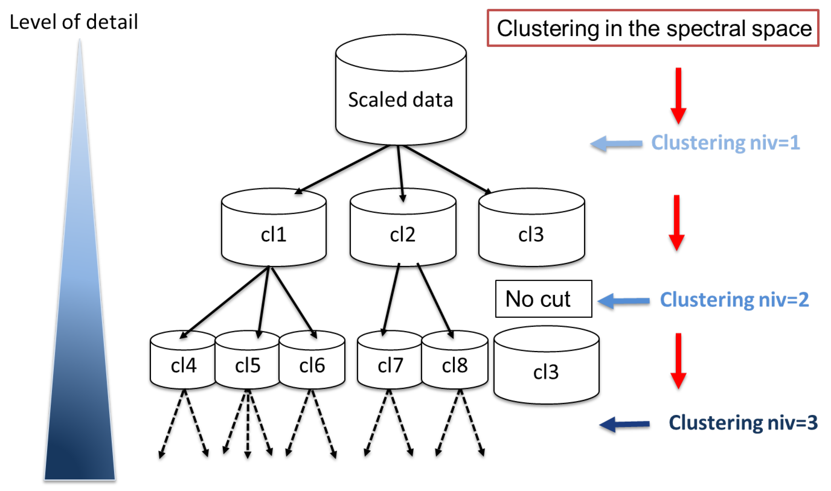
Multi-level spectral clustering. Our M-SC algorithm is a divisive spectral clustering approach use to build a multilevel implicit segmentation of a multivariate dataset [
11]. The first level is a unique cluster with all data. At each level, observations from a related cluster are cut by SC-PAM with K computed from the maximal spectral eigengap. The spectral-PAM algorithm is detailed in Reference [
11]. Here, we add a no-cut criterion (
) for homogeneous clusters according to the silhouette index. (Algorithm 1, (
Figure 1)).
The iterative segmentation of a cluster stops by not-cut criterion when it is well isolated from other clusters and has a good internal cohesion. Indeed, a cluster can be isolated at the first level. However, in the first version of the algorithm, it was systematically subdivided into deeper levels. The deeper levels thus allowed identifying clusters with extreme event characteristics but they over-segmented the more generic clusters.
This criterion is based on the Silhouette Index. Thus, the value of the silhouette of each cluster defines the conditions for stopping the segmentation. If this value is high, that is, higher than it means that our cluster is sufficiently related (i.e., point are close enough to be part of the same set) and thus sufficiently representative. In this case, the segmentation will be stopped for this cluster. Conversely, the segmentation will continue if the Silhouette of the cluster is less than .
should be tuned for the application resolution needs, knowing that the closer the Silhouette Index is to 1, the more the cluster is well-formed and well isolated. For all experiments in this paper, the stop criterion
is set at 0.7; this value is a good compromise between having well-formed cluster and extreme pattern/events.
| Algorithm 1 Multi-Level Spectral Clustering with no-cut stop criterion |
Require: X, NivMax, Kmax, sil.min, W definition of a Gram matrix
Variables : W, cl, sil, clusterToCut = 1, niv = 1, stop = false, groups, k
# Initialisation
cl[n, niv] = 1 matrix of
# Clusterings by level
while (stop! = false) do
for k in clusterToCut do
Compute similarity W of cl[n,niv] = k}
groups = Spectral-PAM(W, Kmax = card(X’))
cl[n, niv] = k, cl[n, niv + 1]= groups+card(clusterToCut) + 1
end for
# computation of silhouette of the new sub-clusters
clusterToCut = {} # empty vector
for k ∈ unique(cl[n, niv + 1]) with n ∈ [1,…,N] do
sil = silhouette() # means of point silhouette
if sil<sil.min then
clusterToCut clusterToCut,k} # insertion
end if
end for
stop = ((niv + 1)≥NivMax (card(clusterToCut) == 0)
niv = niv + 1
end while
return matrix of niv |
3. Comparison Protocol
This work aims to comparing the ability of the above mentioned methods to propose an effective clustering as a first labelling. This section details labelled datasets, the tuning of each method should this step be required, and the list of performance metrics.
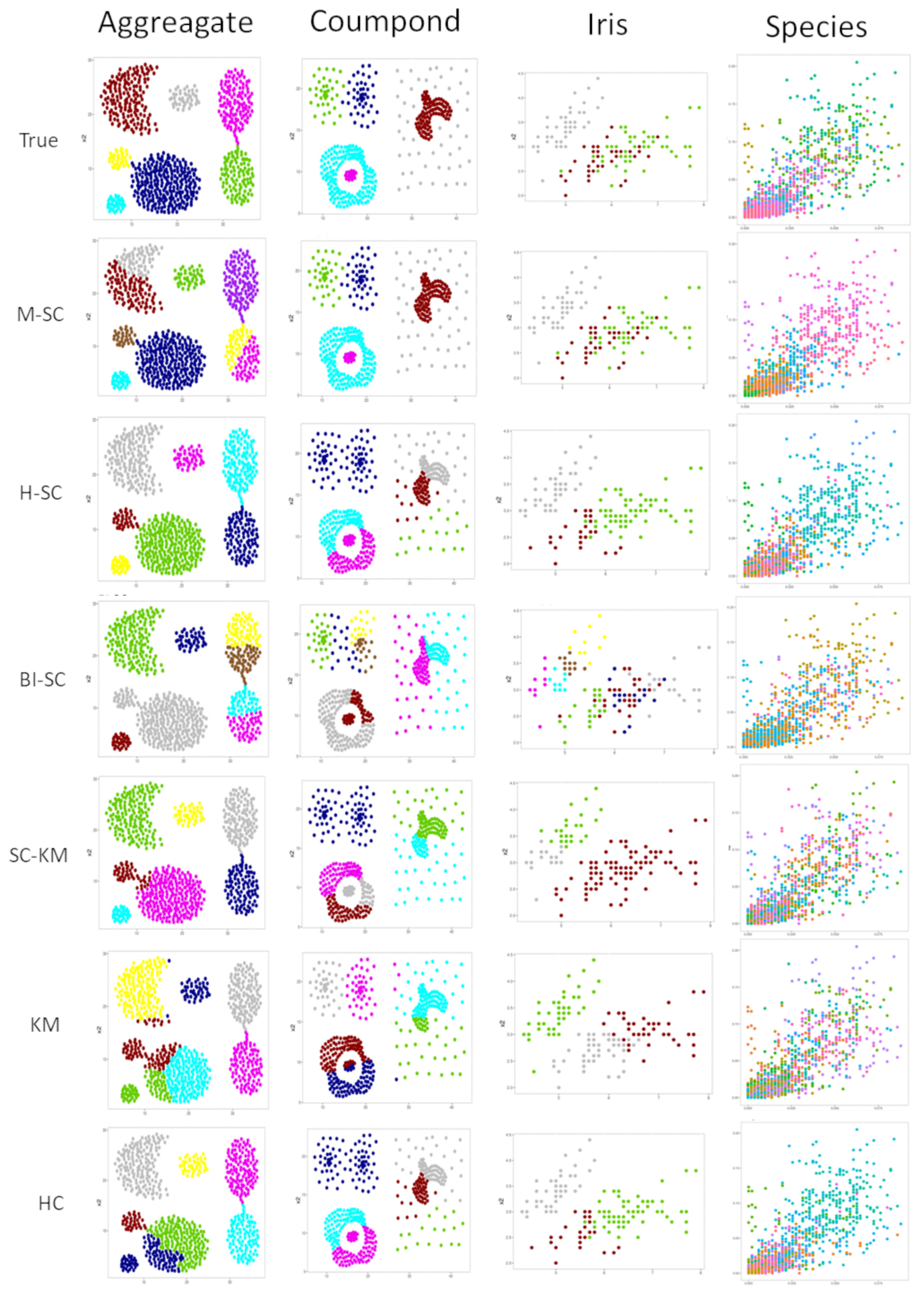
Dataset summary. For pattern discovery and time series segmentation, both selected artificial and experimental cases are briefly described in (
Table 1). From UCI benchmark [
15], two artificial datasets (“Aggregate” and “Compound”) and two experimental ones (“Iris and Species”) are chosen for their geometric characteristics. “Aggregate” has relative simple patches and “Compound” has nested patches, which are both clearly separated. They have respectively six and seven classes and both have two attributes. “Iris” and "Species" have more connected classes. Iris is a simple case because it only has three categories of plants with 50 observations per class, whereas Species has 100 classes with 16 observations per class.
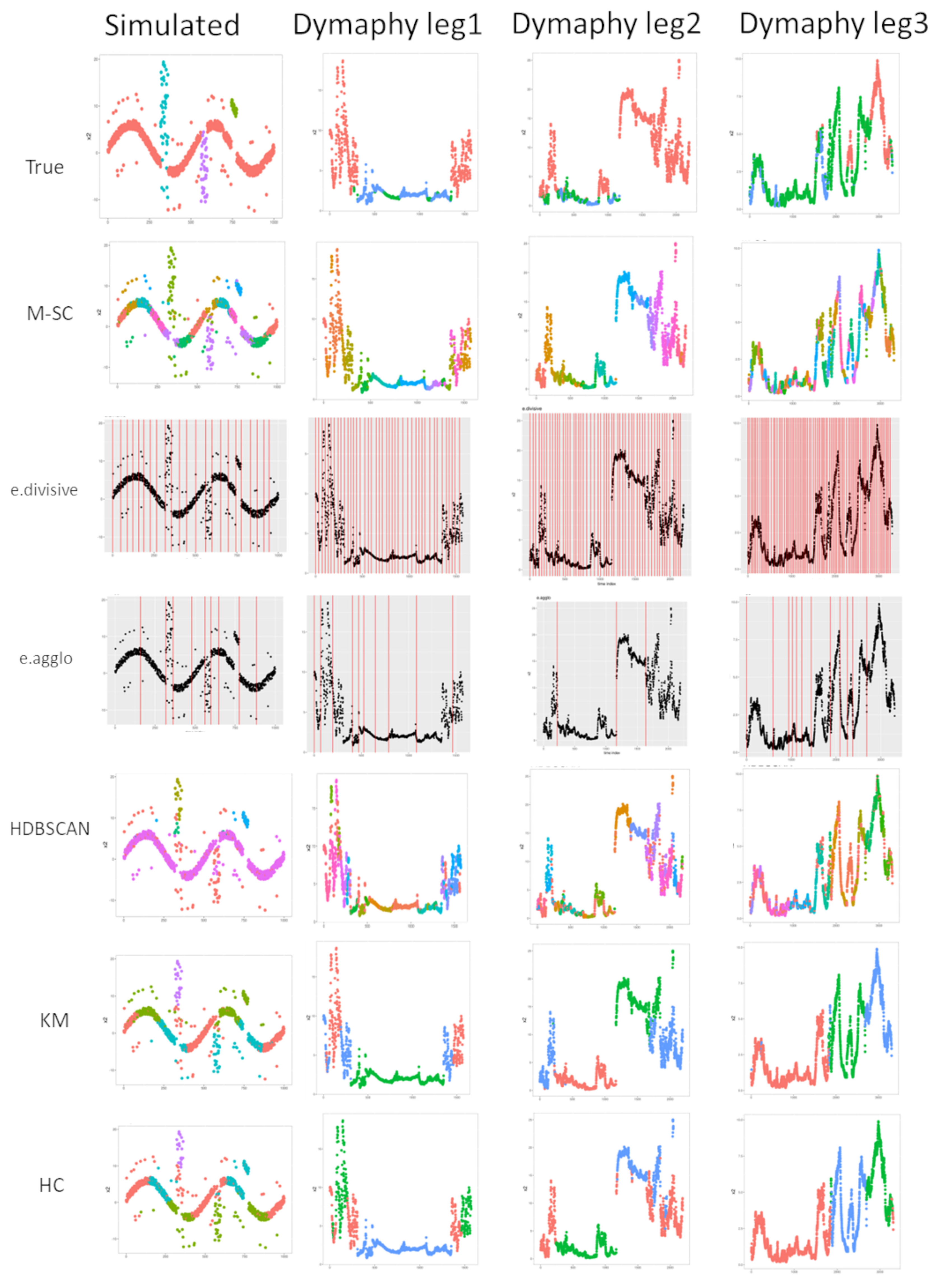
For time series segmentation, the ”Simulated” dataset was built and an experimental dataset from a cruise campaign was used. Simulated is composed of 3 signals based on 3 sinus global-shapes (gs) on which three short events have been inserted: two peaks and one offset (described in Reference [
11]). For the experimental dataset provided by DYPHYMA program [
16,
17], we used the Pocket Ferry Box data (PFB), coupled with the four algae concentrations from a multiple-fixed-wavelength spectral fluorometer (Algae Online Analyser [AOA], bbe Moldaenke). The aim of this last dataset is to identify contrasting water masses based on their abiotic and biotic characteristics (details in Reference [
17]). Each dataset is of dimension N observations × D features. The features are only the explicative variables like environmental parameters for "DYPHYMA" dataset. Time and spatial dimension are not included in clustering step.
Data processing and parameter tuning. Firstly, all dataset X have normalised to avoid the impact of varying feature ranges in the clustering process. Zelnick and Perona locally adapted gaussian kernel with the 7th neighbours sigma distance in the similarity. For M-SC, min.points is defined at 7. Direct spectral methods and M-SC and H-SC are based on Laplacian. So, all functions are computed with their default setting. But some parameters must be defined to choose the number of clusters (K). K is fixed to the ground-truth class number of direct approaches, so . Tree cut in the hierarchical methods (HC, H-SC) and level of divisive methods (Bi-SC, M-SC) are defined to obtain at least C clusters and, sil.min is fixed at 0.7. For DBSCAN the determination of clusters requires -neighbourhood. It is automatically determined by Unit Invariant Knee (UIK) estimation of the average k-nearest neighbour distance. For species dataset, the 20 principal components are retained to obtain the cumulative sum of 95% explained variance.
Comparison metrics. To assess the performance of each algorithm, two indicators are computed: the total accuracy and #Iso. Then three conventional unsupervised scores are added for interpretation: Adjusted Rand index, Dunn index and Silhouette score [
18].
Total accuracy is the percentage of well-recognised labels according to a given ground truth. It is a ratio of correctly classified observations (true positive) to the total observations. It is defined from the confusion table between the K clusters and C classes after a majority vote. The majority vote principle is applied to assign each cluster K to a class C according to the one that is the most represented.
#Iso is the number of well-isolated patterns, that is, represented by more than half of the true positive observations. This is the number of clusters with greater accuracy than 50 percents.
The Adjusted Rand index (ARI) is the corrected-for-chance version of the Rand Index (RI) available in fossil::adjustedRandIndex [
19]. ARI measures the number of agreements in two partitions (same grouping elements and same separating pairs) over the total number of pairs. Rand Index will never actually be zero. It can yield negative values if the index is less than the expected index.
The Dunn index, clValid:dunn [
20] is a ratio of the smallest distance between observations not in the same cluster to the largest intra-cluster distance. The Dunn index has a value between zero and infinity, and should be maximised. It reflects the data/cluster separability. A Dunn index close to zero shows very connected data, while a large score indicates easily separable data.
The Silhouette score, cluster:silhouette [
21] is a measure of how similar an object is to its own cluster (cohesion) compared to other clusters (separation). A large Silhouette (almost 1) is very well clustered, while a small Silhouette (around 0) means that the observations are connected between two clusters.
All indexes were computed in the raw space whatever the clustering methods used. Low Dunn index and averaged silhouette score from true label show the complexity to isolate each class, especially for DYOHYMA sets, Dunn index computed from the ground-truth labels are around .
4. Clustering Results
Table 2 summarizes the clustering methods that succeed in isolating at least 50% of ground-truth patterns. They are ordered according to first #Iso, the total accucary and then minimum
K to reduce the human labelling task.
Spectral methods succeed in discovering all spatial patterns (#Iso
C) with a high score for hierarchical approaches: they could achieve 100% of accuracy, particularly M-SC except for “species”. For example, within the “coumpound” dataset, M-SC is able to detect nested or overlaped clusters (clusters cyan and pink), while no other method makes the separation (
Figure 2). However, within the “species” dataset, methods including M-SC have low scores and only part of the
C classes are detected It could be explained by the low-class distribution and highly connected clusters (averaged silhouette = 0.1). For the time series segmentation task, hierarchical methods better isolated event patterns, particularly M-SC, e.divisive and HDBSCAN. For ”DYPHYMA-leg3”, none of the algorithms isolated 3 classes. M-SC succeeded in isolating them at level 3 with
and a total accuracy of 93%. This number of clusters to label could be too many and unreasonable for the human expert, but we considered that who can do more can do less. Who can do more can do less.The objective is to offer the expert the possibility to define its own level of relevant expertise based on the best available number of clusters.
Multi-Level Spectral clustering seems to be effective to detect pattern structure in spatial data or time series (
Figure 2 and
Figure 3). The obtained results reveal a good ability for generalisations. However, the no-cut criterion is a sensitive parameter and is not self-sufficient when the connection is too important, like the “species” or “ DYPHYMA-leg3” datasets. Moreover, the deepest level permit to detect a large number of events or patterns but leads to over-segmentation. Human experts should tune M-SC silhouette parameters and levels of clustering according to a compromise between over-segmentation and cluster number for their labelling task. For large databases, the M-SC algorithm could be easily modified to obtain a fast computation process by using a reduced prototype set and an
-nearest neighbour algorithm.
The efficiency of a given method depends on the data distribution hypothesis and capacity to include it. For simple examples, that is, linear or with low connexity data, methods such as KM or HC are relevant. However in our application these direct methods (KM or HC) are less effective for our application because they require non-convexe shapes and linearly separable clusters to be optimal. Also, segmentation by breaking points (e.divisive and e.agglo) are performing when signals have a break between 2 stationary regimes. These breaks are not so obvious in marine data where extreme events are not an intensive variation with the overall signal in mean or variance. DBSCAN and HDBSCAN consider this extreme event often as outliers.
5. Clustering for Labelling
Clustering methods rely solely on data geometry to provide data segmentation. The purpose of this last section is to test their ability to provide a first labelling. So we compare them now with supervised techniques in the task of pattern discovery in time series.
Three basic machine solutions were explored: k-Nearest Neighbours classification (k-nn), Breiman’s Random Forest algorithm (RF) [
22] and a Multi-Layer perceptron (MLP). For comparison, MLP was preferred to Time Delay Neural Networks to be fair with clustering approaches that do not take account time parameters also.
Two training databases per dataset (from 5 to 8 in
Table 1) werre built. The first database represents 20% of the volume of each class in the Table (80% for the test database) and the second 50%. Whatever the training and test base is, it covers all
temporal events. The attributes of an observation in the series are the classifier entries: for the 8th dataset, the input number
I is equal to 18. And
C is the output number of MLP and RF. For k-nn, two k values are chosen.
k is set to 1 to assign the label of the closest observation and then
to obtain a a more unified segmentation (ie. with less than one class singleton among observations of other classes). MLP-1 here has one hidden layer whose neuron number is equal to
and MLP-0 corresponds to linear perceptron (no hidden layer). Random Forest here consists of the vote of 500 trees with
variables randomly sampled as candidates at each split.
The same unsupervised and supervised scores as in
Table 2 are computed on the test databases and reported in
Table 3 in order to compare clustering and classification approaches.
Learning techniques do not over-segment the time series due to the fixed number of their classes.
RF and k-nn are able to isolate events with higher accuracy and so lead to low overlap between them for every dataset and every training cut. MLP-0 and MLP-1 are able to identify the 4 events of the simulated case but they are not efficient for in-situ cases (n = 6–8) due to a lack of observations and unequal classes.
Divisive clustering techniques like M-SC do not suffer from unequal classes and can better to detect events in the series. M-SC reached the same objective of well-isolated pattern number as supervised techniques like RF or k-nn. ARI and connectedness scores are highly dependent on the number of classes. In the supervised case, with a fixed K-number and computed from the test database only, ARI scores are higher than those of clustering approaches. However, the connectedness indices are not better.
This study has shown that the Multi-level Spectral Clustering approach is a promising way to assist an expert in a labelling task for both spatial data and time series. M-SC also provides a deep hierarchy of labels depending on the desired depth of interpretation.
6. Conclusions
In marine ecology, understanding and forecasting events and environmental states is crucial for many applications, so artificial intelligence systems should especially to facilitate understanding of ecosystem processes and dynamics. It is also important for evaluation of ecosystem health in order to qualify environmental status and to put adaptative strategies to reduce the anthropogenic pressure on marine ecosystems. So, integrate and multi-scale optimal approaches are therefore needed to effectively monitor complex and dynamic ecosystems. So, the correct detection of environment state in no-linear multivariate dataset required the right numerical methodology. It is essential to optimise the processing in order to extract relevant information for stakeholders. We propose, a Multilevel Spectral Clustering (M-SC) was proposed multivariate time series into general patterns up to extreme events by unsupervised way and demonstrate this algorithm outperforms existing algorithms for this task.
In this case, we improved the processing of the spectral method by adding hierarchical and density approaches. The deep architecture allows processing without losing key information for the detection of extreme events. In fact, this hierarchy allows eliminating the strong contributions of structuring variables linked to trends in early levels and general seasonal cycles and, to observe more specific environmental states at deeper levels while preserving all the explanatory variables. Then the no-cut criterion based on density and connexity indexes facilitates heterogeneous clustering. This allows the identification of classes of different sizes and duration. This is a significant advantage when studying processes whose phenology is highly variable, as in the case of harmful algae blooms. Thus, experts can use this criterion to find a compromise between over-segmentation and the number of classes necessary for their labelling task.
These different aspects are not present or only partially present in other clustering algorithms. The tests performed on artificial and experimental datasets with high local connexity between events and global-shape signals showed that the M-SC architecture can segment several kinds of shapes with which related algorithms struggle. M-SC often offers the most efficient segmentation. These results also reveal a good result for first labelling, it is close to the supervised machine learning techniques and includes a reasonable number of clusters with coherent structures.
Therefore, M-SC multilevel implicit segmentation will enable the implementation of nested approaches and to optimise extraction of knowledge when considering data covering different scales (temporal, frequency or spatial).
The extended M-SC approach seems well adapted for segmentation of time series or spatial datasets with coherent patterns that could appear several times or once. It combines the segmentation and clustering steps in the process and suggests different scales of interpretation, including a good detection of extreme events for an integrated observing approach.
However, M-SC has several limitations. The major drawback is that it requires a complete dataset: observations with no missing values (NA). In the case of NA values, data would not be assigned to cluster and could affect the clustering step. It is important to align the data. The choice of similarity and Laplacian operator was not studied here. The choice of Similarty matrix W or Laplacian definition L could affect the results and depend on the application. Furthermore, SC computation could be difficult for large datasets and in this case it will be replaced by Fast-NJW spectral algorithm based on a clustering after sampling (by a vector quantization). Another important point is sil.min parameter tuning. sil.min could be not been strong enough for applications with events or geographical pattern composed of very few observations.
We believe that the M-SC approach could be used for other marine applications (data from Ferry Box, gliders, etc.) and also for other applications when needing to segment data series and to identify general patterns and specific events without any a priori knowledge. For example, (I) The method could allow the characterisation of environmental states and associated phytoplankton assemblages. This would enable ecosystem dynamics studies and a better understanding at the environmental forcing (nutrient inputs, storms, ect) on multiple spatial and temporal scales. It should be of importance for eutrophication monitoring and Harmful Algal Blooms (HABs) forecasting. (II) Applied to Ferry Box data, it could permit the detection and characterisation of eco-regions and associated phytoplankton communities. This would make it possible to propose global or local assessments and could help in decision-making within the framework of the project to establish ecological status of marine waters(DCSMM, OSPAR conventions) or within the framework of the structuring of observation networks (H2020 JERICO-S3 project). From machine learning methods, it could enable the implementation of real-time sampling strategies during sea campaigns. (III) The classification could also be used to detect sensor failures and measurement anomalies on automated measuring stations. An alert system could be set up, which would speed up maintenance operations.
Author Contributions
Conceptualization, K.G., É.P.-C. and A.L.; methodology, K.G. and É.P.-C.; software, K.G. and É.P.-C.; validation, A.L., É.P.-C. and A.B.; formal analysis, K.G.; investigation, A.L., É.P.-C. and A.B.; resources, A.L.; data curation, K.G.; writing–original draft preparation, K.G., É.P.-C., A.B. and A.L.; writing–review and editing, K.G., É.P.-C., A.B. and A.L.; supervision, A.L. and É.P.-C.; project administration, A.L. and É.P.-C.; funding acquisition, A.L. All authors have read and agreed to the published version of the manuscript.
Funding
This work has been financially supported (1) by the European Union (ERDF), the French State, the French Region Hauts-de-France and Ifremer, in the framework of the project CPER MARCO 2015–2020 (Grant agreement: 2016_05867 et 2016_05866), and (2) by the JERICO-S3 project which is funded by the European Commission’s H2020 Framework Programme under grant agreement No. 871153. Project coordinator: Ifremer, France. Kelly Grassi’s PhD is funded by WeatherForce as part of its R & D program “Building an Initial State of the Atmosphere by Unconventional Data Aggregation”.
Conflicts of Interest
The authors declare no conflict of interest.
References
- Van Hoan, M.; Huy, D.; Mai, L.C. Pattern Discovery in the Financial Time Series Based on Local Trend. In Advances in Information and Communication Technology; Springer: Cham, Switzerland, 2017; Volume 538. [Google Scholar] [CrossRef]
- Längkvist, M.; Karlsson, L.; Loutfi, A. A review of unsupervised feature learning and deep learning for time-series modeling. Pattern Recognit. Lett. 2014, 42, 11–24. [Google Scholar] [CrossRef] [Green Version]
- Emonet, R.; Varadarajan, J.; Odobez, J.M. Temporal Analysis of Motif Mixtures Using Dirichlet Processes. IEEE Trans. Pattern Anal. Mach. Intell. 2014, 36, 140–156. [Google Scholar] [CrossRef] [PubMed] [Green Version]
- Dias, J.; Vermunt, J.; Ramos, S. Clustering financial time series: New insights from an extended hidden Markov model. EJOR-Eur. J. Oper. Res. 2015, 243, 852–864. [Google Scholar] [CrossRef] [Green Version]
- Tsinaslanidis, P.; Kugiumtzis, D. A prediction scheme using perceptually important points and dynamic time warping. Expert Syst. Appl. 2014, 41, 6848–6860. [Google Scholar] [CrossRef]
- Kuswanto, H.; Andari, S.; Oktania Permatasari, E. Identification of Extreme Events in Climate Data from Multiple Sites. Procedia Eng. 2015, 125, 304–310. [Google Scholar] [CrossRef] [Green Version]
- Sharma, P.; Suji, J. A Review on Image Segmentation with its Clustering Techniques. Int. J. Signal Process. Image Process. Pattern Recognit. 2016, 9, 209–218. [Google Scholar]
- Ng, A.; Jordan, M.; Weiss, Y. On Spectral Clustering: Analysis and an Algorithm; MIT Press: Cambridge, MA, USA, 2001; pp. 849–856. [Google Scholar]
- Shi, J.; Malik, J. Normalized Cuts and Image Segmentation. IEEE Trans. Pattern Anal. Mach. Intell. 2000, 22, 888–905. [Google Scholar] [CrossRef] [Green Version]
- Sanchez-Garcia, J.; Fennelly, M.; Norris, S.; Wright, N.; Niblo, G.; Brodzki, J.; Bialek, J.W. Hierarchical Spectral Clustering of Power Grids. IEEE Trans. Power Syst. 2014, 29, 2229–2237. [Google Scholar] [CrossRef] [Green Version]
- Grassi, K.; Caillault, E.P.; Lefebvre, A. Multi-level Spectral Clustering for extreme event characterization. In Proceedings of the MTS IEEE OCEANS 2019, Marseille, France, 17–20 June 2019. [Google Scholar]
- Rousseeuw, K.; Poisson Caillault, É.; Lefebvre, A.; Hamad, D. Hybrid Hidden Markov Model for Marine Environment Monitoring. IEEE JSTARS-J. Sel. Top. Appl. Earth Obs. Remote Sens. 2015, 8, 204–213. [Google Scholar] [CrossRef] [Green Version]
- Ester, M.; Kriegel, H.; Sander, J.; Xu, X. A density-based algorithm for discovering clusters in large spatial databases with noise. KDD Proc. 1996, 96, 226–231. [Google Scholar]
- James, N.; Matteson, D. ecp: An R Package for Nonparametric Multiple Change Point Analysis of Multivariate Data. J. Stat. Softw. 2015, 62, 1–25. [Google Scholar] [CrossRef] [Green Version]
- Dua, D.; Graff, C. UCI Machine Learning Repository; University of California, School of Information and Computer Science: Irvine, CA, USA, 2017. [Google Scholar]
- DYPHYMA Dataset. Continuous Phytoplankton Measurements during Spring 2012 in Eastern Channel. 2012. Available online: https://sextant.ifremer.fr/record/5dbafe69-81cf-4202-b541-9f8b564fa6f9/ (accessed on 12 September 2020).
- Lefebvre, A.; Poisson-Caillault, E. High resolution overview of phytoplankton spectral groups and hydrological conditions in the eastern English Channel using unsupervised clustering. Mar. Ecol. Prog. Ser. 2019, 608, 73–92. [Google Scholar] [CrossRef]
- Zhao, Q. Cluster Validity in Clustering Methods; University of Eastern Finland. Dissertations in Forestry and Natural Sciences: Joensuu, Finland, 2012; no 77; ISSN 1798-5676. [Google Scholar]
- Vavrek, M.J. Fossil: Palaeoecological and palaeogeographical analysis tools. Palaeontol. Electron. 2011, 14, 16. [Google Scholar]
- Brock, G.; Pihur, V.; Datta, S.; Datta, S. clValid: An R Package for Cluster Validation. J. Stat. Softw. Artic. 2008, 25, 1–22. [Google Scholar] [CrossRef] [Green Version]
- Maechler, M.; Rousseeuw, P.; Struyf, A.; Hubert, M.; Hornik, K. Cluster: Cluster Analysis Basics and Extensions; R Package Version 2.1.0; Brown Walker Press: Boca Raton, FL, USA, 2018. [Google Scholar]
- Breiman, L. Random Forests. Mach. Learn. 2001, 45, 5–32. [Google Scholar] [CrossRef] [Green Version]
© 2020 by the authors. Licensee MDPI, Basel, Switzerland. This article is an open access article distributed under the terms and conditions of the Creative Commons Attribution (CC BY) license (http://creativecommons.org/licenses/by/4.0/).


