Practical Prediction of the Boil-Off Rate of Independent-Type Storage Tanks

Abstract

Because environmentally-friendly fuels such as natural gas and hydrogen are primarily stored in the form of cryogenic liquids to enable efficient transportation, the demand for cryogenic fuel (LNG, LH) ships has been increasing as the primary carriers of environmentally-friendly fuels. In such ships, insulation systems must be used to prevent heat inflow to the tank to suppress the generation of boil-off gas (BOG). The presence of BOG can lead to an increased internal pressure, and thus, its control and prediction are key aspects in the design of fuel tanks. In this regard, although the thermal analysis of the phase change through a finite element analysis requires less computational time than that implemented through computational fluid dynamics, the former is relatively more error-prone. Therefore, in this study, a cryogenic fuel tank to be incorporated in ships was established, and the boil-off rate (BOR), measured considering liquid nitrogen, was compared with that obtained using the finite element method. Insulation material with a cubic structure was applied to the cylindrical tank to increase the insulation performance and space efficiency. To predict the BOR through finite element analysis, the effective thermal conductivity was calculated through an empirical correlation and applied to the designed fuel tank. The calculation was predicted to within 1% of the minimum error, and the internal fluid behavior was evaluated by analyzing the vertical temperature profile according to the filling ratio.

1. Introduction

The International Maritime Organization (IMO) has established emission control areas (ECAs) in the North and Baltic seas to improve the air quality and limit the presence of low-quality residual fuel (or heavy fuel oil, HFO). Marine emission legislations such as the Tier III requirements of the revised MARPOL Annex VI mandate ships to reduce NOx emissions, with an objective of reducing the greenhouse gas emissions by 20% and 50% until 2020 and 2050, respectively [1,2].

Owing to these requirements, alternative fuels such as natural gas and hydrogen gas are being used instead of HFO as ship propellants. In particular, liquefied natural gas (LNG), whose volume can be reduced by cooling natural gas to 110 K, is environmentally friendly as it can reduce the energy efficiency design index by 20% [3,4,5]. It has been predicted that ships to transport LNG and those that employ LNG as a fuel will undergo accelerated development by 2035 [6,7]. Nevertheless, to enable the efficient storage and transportation of LNG, the storage systems must be insulated to maintain the temperature. Moreover, in LNG storage tanks, boil-off gas (BOG) is generated owing to the vaporization of liquefied gas as the external heat is ingressed. The BOG can deteriorate the structural intensity owing to the pressurization of the storage system. Therefore, this gas is usually purged and subjected to reliquefaction [8,9,10]. However, because this process results in economic losses, it is desirable to predict and minimize the amount of BOG in the design stage.

LNG tanks can be categorized into membrane and independent types. Membrane-type tanks are mainly implemented in the LNG cargo hold of carriers instead of as fuel tanks [11]. IMO A and B type tanks, which are independent tanks, can resist the sloshing load owing to their stiff structure. Moreover, such tanks have a secondary barrier to prevent the leakage of liquids and equipment to process the BOG [12,13]. Therefore, such tanks are advantageous in terms of inspection and repair capacities. In contrast, type C independent tanks are designed as pressure tanks with a high inner pressure and without the equipment for BOG processing (

Table 1. IMO independent type tanks for LNG ship [14].

Type	Prismatic Type	MOSS Type	Cylindrical Type
IMO Tank Type	Type A	Type B	Type C
Schematic structure
Secondary barrier	Complete	Partial	No requirements
Characteristic	Fully refrigerated at atmospheric pressure	Fully refrigerated at atmospheric pressure	Pressurized at ambient or lower temperature
Notes	For small vessels less than approx. 20,000 m3 capacity	For large vessels	For LNG carriers

) [14]. Such tanks are mainly used as fuel tanks for LNG-propelled ships due to their low space efficiency.

In the context of the expansion of the ECAs and more stringent environmental regulations, it is necessary to examine small vessels sailing along the coast as well as large vessels. The heat transfer rate of small pressurized liquid tanks is larger than that of a large liquid tank owing to the larger surface area to volume ratio of the former [15]. However, most of the existing research pertains to large cargo holds [16,17,18], and the research on fuel tanks is limited. In particular, the research on cryogenic fuel tanks for small vessel applications is inadequate.

Several researchers have employed computational fluid dynamics (CFD) to examine the physical phenomena pertaining to the various types of BOG occurrences [19,20,21,22,23]. However, the boil-off rate (BOR) calculations are challenging owing to the complex heat transfer and fluid flow involved, owing to which, the calculation time to ensure the convergence in the case of small steps is extremely large. In particular, it is difficult to set the initial temperature considering the filling ratio (FR) of a tank because the temperature changes continuously owing to the liquid evaporation, and heat convection occurs in a complex manner [24]. Many researchers performed finite element analyses (FEA) based on the conduction model to address the complex convection behavior and reduce the calculation time compared to that required for CFD computations [25,26,27,28].

Considering these aspects, in this study, cryogenic fuel storage tanks for small ships were designed according to the rules of the IMO and ship classification, and the amount of generated BOG was measured experimentally. Based on the measurement data, a numerical analysis was performed to predict the BOR of other small tanks. The BOG was measured considering the change in mass of the cryogenic liquid inside the tank, and the numerical analysis was performed using a commercial FEA code. Variables that are boundary conditions in the process of numerical analysis were derived by empirical correlation. In the verification process of an experiment, it is possible to predict the results or variables used for calculation by the method by recent deep learning. This method can be applied to predict the phase change of cryogenic fluid, and there are cases applied to equipment such as heat exchangers [29,30]. However, in this study, BOR prediction by finite element analysis was performed, and data were verified through comparison with experimental results.

2. Experiment Details

2.1. Design and Manufacturing of the Experiment Structure

IMO type C independent tanks consist of an inner pressure tank and insulation to prevent heat ingress. In the case of the pressure tank, hemispherical parts are attached at both ends of a cylindrical tank in the horizontal orientation to resist the internal pressure. The cylindrical and hemispherical parts are manufactured using stainless steel 304L, which demonstrates excellent characteristics under cryogenic temperatures [31].

For fuel tanks operating at cryogenic temperatures, the thickness of the inner wall should be determined considering the thermal stress and internal pressure. The thickness of internal tanks under pressure is regulated by the international gas carrier (IGC) code and Korea Register (KR) [32]:

$$\begin{array}{c}{t}_c=\frac{PD}{2fJ-1.2P}+1.0\\ t_h=\frac{PR}{2fJ-0.2P}+1.0\end{array}$$

(1)

where t_c and t_h denote the minimum thickness of the cylinder plate (mm) and hemisphere plate (mm), respectively; P is the design pressure (MPa), D is the diameter of the cylinder plate (mm); R is the radius of the hemisphere (mm); f is the maximum allowable stress (MPa); and J is the weld efficiency.

The IGC code classifies tanks with an operating pressure of 0.2 MPa or higher as IMO type C independent tanks. However, as the BOR generally decreases with an increase in the internal pressure, most storage containers currently operate in environments greater than 0.5 MPa [33]. Therefore, the design pressure of the tank produced in this study was set to range from 1 MPa to 1.5 MPa, and the thickness of the pressure tank was set as 4 mm.

The insulation system was made of polyurethane foam (PUF) and manufactured as a cuboid box. In general, a saddle support is installed in the case of the conventional cylindrical tank; however, such support is unnecessary when manufacturing the support as a cuboid box, and this aspect can help prevent heat loss. PUF, synthesized with polyol and isocyanate [34,35], was expanded in a plywood box mold. The density of the applied PUF was 96 kg/m³, to ensure the required insulation performance. The specifications of the tank are listed in

Table 2. Specification for IMO Type C tank.

	IMO Type C Tank
Dimension	Length (mm)	1414
	Breadth (mm)	624
	Height (mm)	612
Pressure	Design (MPa)	1.5
	Operating	-
Insulation thickness	Maximum (mm)	224
	Minimum (mm)	100
Internal volume (m3)		0.127
Test fluid		Liquid nitrogen

.

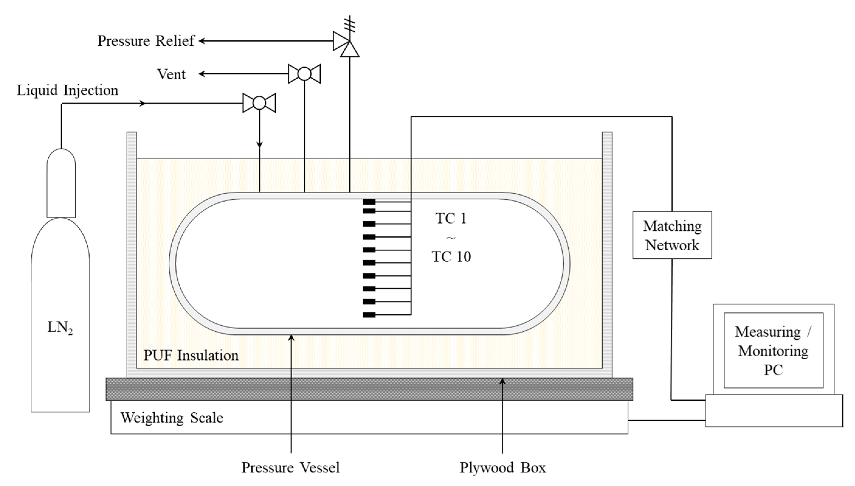
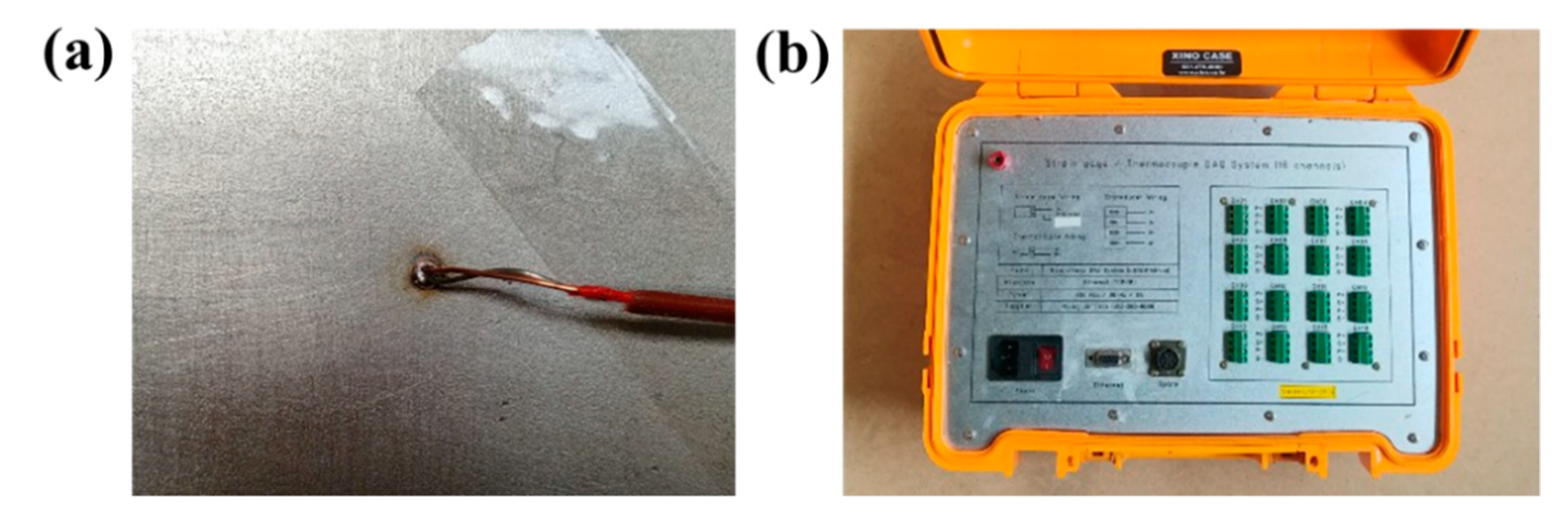
2.2. Experimental Apparatus and Procedure

Thermocouples (TCs) and a weighing scale (WS) were sed to measure the internal temperature distributions and BOR of the cuboid insulation type C tank. As shown in Figure 1, the fuel storage tank was filled with liquid nitrogen instead of cryogenic fuel to ensure safe operation. The WS (CAS Corporation, Korea) least count was 0.1 kg, and data were obtained every 10 s considering the period of the experiment. T-type TCs, which are suitable for cryogenic temperatures, were attached to the surface of the inner tank through spot welding. Subsequently, the TCs were connected to the data acquisition (DAQ) system, and the data were transferred to the main computer (Figure 2). The devices were attached at 10% FR intervals to determine the temperature distribution at the FRs at the 10% to 90% height point and further welded at the location of the maximum load (98%) after the 90% location. To avoid the damage of the TCs during the foaming of polyurethane, a coating was applied on the welded area, and an aerogel mat was placed on the inner tank to protect the tank (Figure 3).

In the experiment, the amount of spontaneous vaporization was measured by fully charging the tank fully through the pressure difference of the liquid nitrogen at a certain pressure. Ventilation valves and pressure relief valves were installed in addition to the inlet valves to ensure sufficient discharge at pressures above 1.5 MPa. Each valve operated independently, and the vent valve was installed at the 98% level to prevent 100% filling.

Pre-cooling was performed to prevent the occurrence of structural defects caused by the difference in the thermal expansion coefficient owing to the rapid temperature change in the tank. In general, the cryogenic cargo hold for ships is implemented for one or two days [36]; however, in this study, a period of 6 h was considered, to allow the temperature to converge, considering the size of the tank.

3. Numerical Analysis of the Heat Transfer

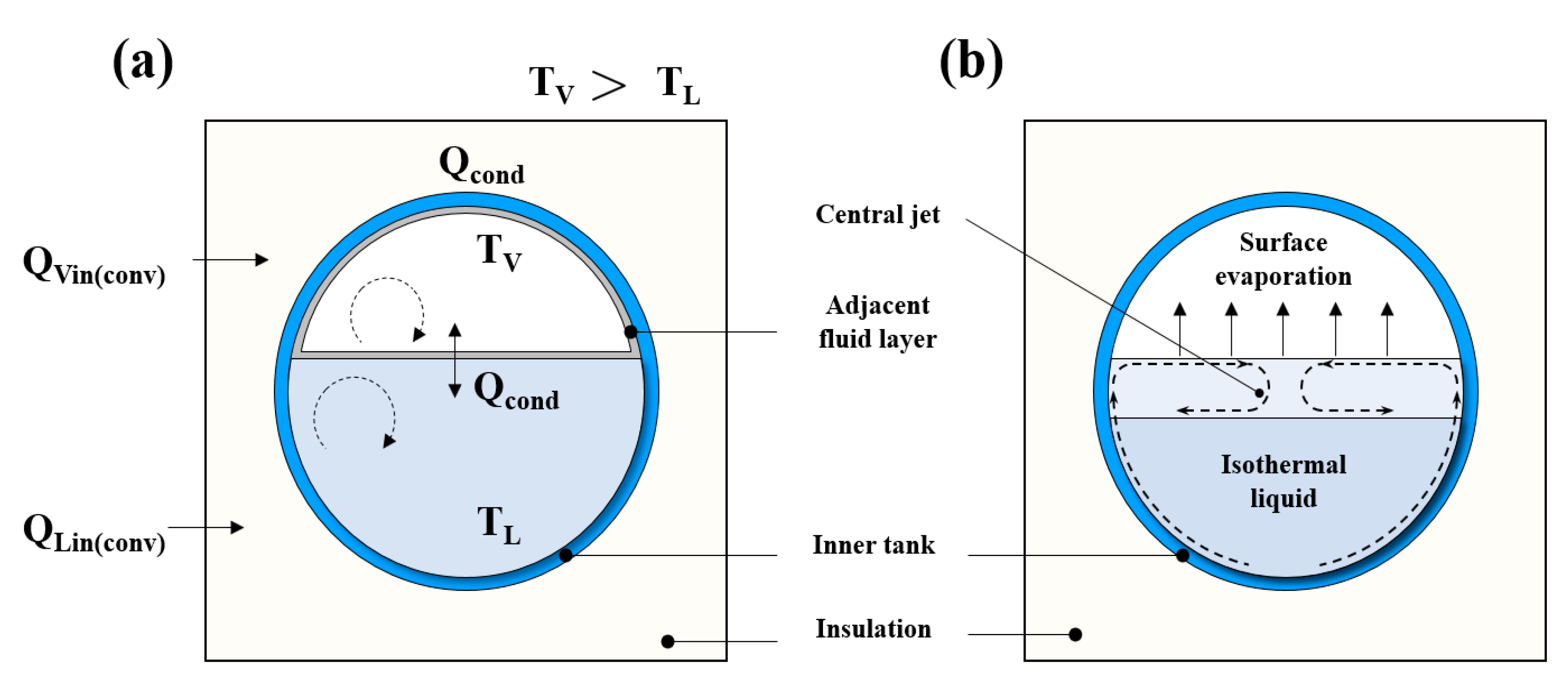
3.1. Theoretical Model

The BOR of the IMO independent-type C fuel tank was calculated using a thermal conductivity model. In general, the BOR is defined as the amount of liquid evaporated through vaporization during the day relative to the total load in the storage tank. Over time, external heat enters the cryogenic tank (Q), which causes the BOR to increase. The BOR can be calculated as follows:

$$BOR=\frac{Q_{in}\times 24\times 3600\times 10}{V\times \rho \times H_{vap}}\times 100$$

(2)

where Q_in is the heat inflow from the outside, and ρ and H_vap denote the density of the cryogenic fluid and latent heat, respectively.

As shown in Figure 3, the fluid heat transfer in a liquefied gas storage tank in a static state can be interpreted from two perspectives. First, as shown in Figure 3a, assuming that the inner fluid is a conduction model, the BOG generation can be interpreted as conduction to the inner fluid through the heat from the external environment. In the case shown in Figure 3b, the fluid dynamic behavior inside the tank is considered. A stable isothermal distribution exists in the lower part of the liquid state; however, a thermal stratification section appears due to the temperature difference in the upper part, and convection occurs owing to the temperature difference [37,38,39]. The vapor space in the tank rises upwards, the evaporation continues, and the density increases, in a process known as weathering [4,40]. In the domain of vertical storage tanks, considerable research has been performed on the thermal stratification section owing to the uniform cross-section [41,42]; nevertheless, a horizontal shape has not been applied to ships owing to the geometrical differences.

Considering these aspects, in this study, the analysis was performed using the thermal conductivity model. However, the convection phenomenon of the upper tank due to BOG can cause significant errors when calculating with the thermal conductivity model. Therefore, effective thermal conductivity was applied to increase the precision of the BOR prediction. The effective thermal conductivity was applied to the adjacent layer of gas and inner tank internal, and the heat inflow was calculated by using the empirical correlation for the effective thermal conductivity to reduce the error. The adjacent layer was assumed to be a shell and calculated by considering the geometry and FR of the tank.

3.2. Effective Thermal Conductivity of the Interface of the Liquid and Vapor

The governing equations used in the numerical analysis were derived from the energy conservation equations, and the transfer rate equations were applied. The resulting heat diffusion equation can be expressed as follows:

$$\frac{\partial }{\partial x}\left(k\frac{\partial T}{\partial x}\right)+\frac{\partial }{\partial y}\left(k\frac{\partial T}{\partial y}\right)+\frac{\partial }{\partial z}\left(k\frac{\partial T}{\partial z}\right)=\rho c_p\frac{\partial T}{\partial t}$$

(3)

where k is the thermal conductivity, c_p is the specific heat capacity, ρ is the density, and T is the reference temperature.

As the hydrodynamic behavior is not considered in the thermal conductivity model, the temperature of the fluid boundary layer can be considered to be equivalent to that of the adjacent part (no-temperature jump condition). This condition can satisfy the no-slip condition, according to which, the velocity of the fluid in the boundary layer is zero [26]. These conditions can be expressed as in Equation (4):

$$\begin{array}{c}{\dot{q}}_{conv}=h\left(T_{adj}-T_{BOG}\right)=-k_{conv}\left(\frac{\partial T}{\partial n}\right)\\ {\dot{q}}_{conv}={\dot{q}}_{cond}=-k_{fluid}{\frac{\partial T}{\partial y}}_{y=o}\end{array}$$

(4)

where h is the heat transfer coefficient of the BOG, subscript adj represents the adjacent fluid layer of the gas, and n is the normal vector.

The heat from the outside of the tank leads to convection, and the effective thermal conductivity is applied to the adjacent fluid layers to account for this aspect in the conduction model. The effective thermal conductivity can be expressed as in Equation (5):

$$k_{eff}=kNu$$

(5)

$$Nu=\frac{hL}{k}$$

(6)

Here, Nu is the Nusselt number, defined as the ratio of the convection coefficient to the conduction coefficient.

The convection coefficient depends on the structure; therefore, empirical correlations are applied to obtain the corresponding value. Migliore et al. defined the Nusselt number as in Equation (7) [4]:

$$Nu=0.116R{a}^{0.32}$$

(7)

$$Ra=Gr\cdot Pr$$

(8)

Ra, that is, the Rayleigh number, is derived from the dimensionless number defined in Equations (9) and (10):

$$Gr=\frac{g\beta \left(T_L-T_G\right)L_c{}^3}{v^2}$$

(9)

$$Pr=\frac{\mu C_p}{k}$$

(10)

where Gr and Pr represent Grashof Number and Prandtl Number, respectively. Here, g is the gravitational acceleration, β is the thermal expansion coefficient, Lc is the characteristic length, and ν and μ represent the kinetic and dynamic viscosity coefficients, respectively.

In general, as the FR decreases, the temperature difference of the gas layer increases, and the Grashof number increases, corresponding to an increase in the effective thermal conductivity. Figure 4 shows the BOR calculation process flow through the numerical analysis. In this study, the temperature obtained experimentally and the effective thermal conductivity for each FR of the tank were used as the input values. The BOR was calculated by solving the heat transfer equation, and a no-temperature jump condition and no-slip condition were implemented considering the heat conduction model.

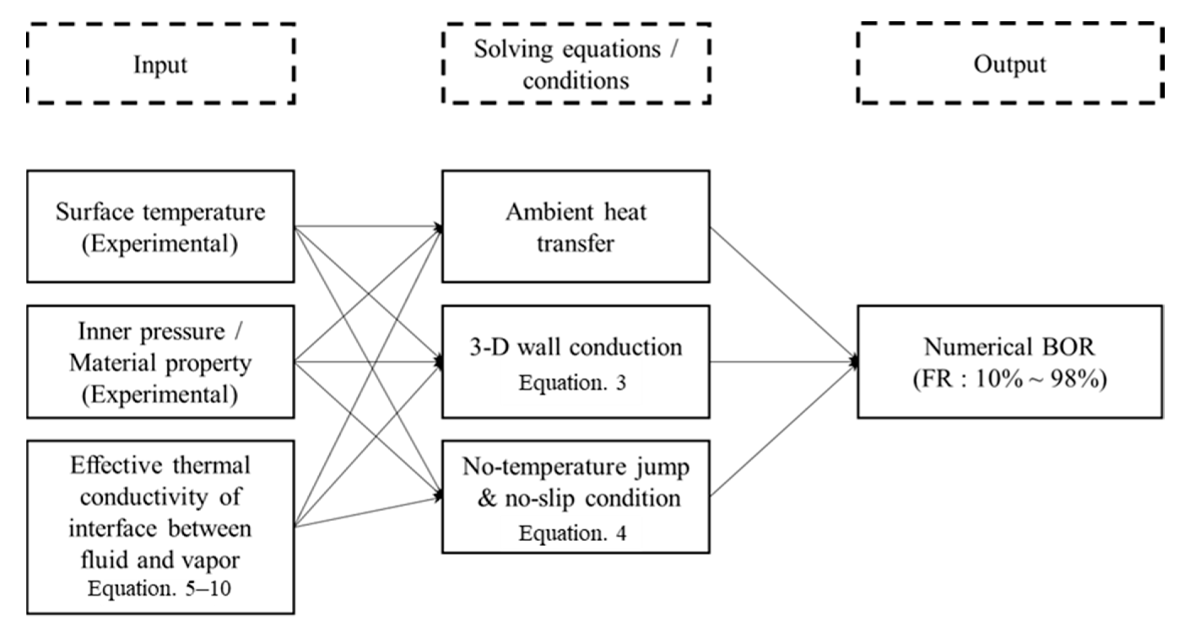
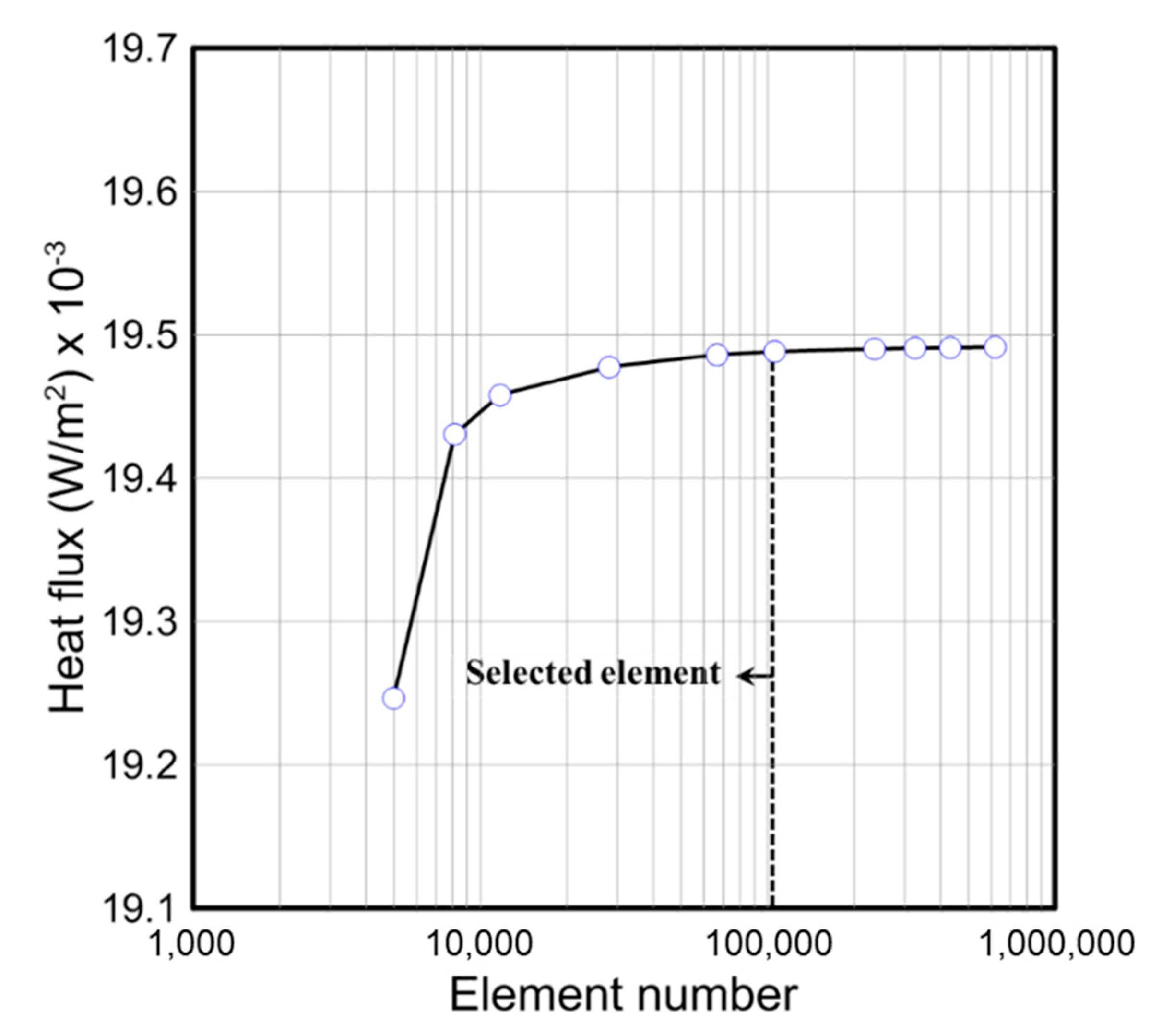
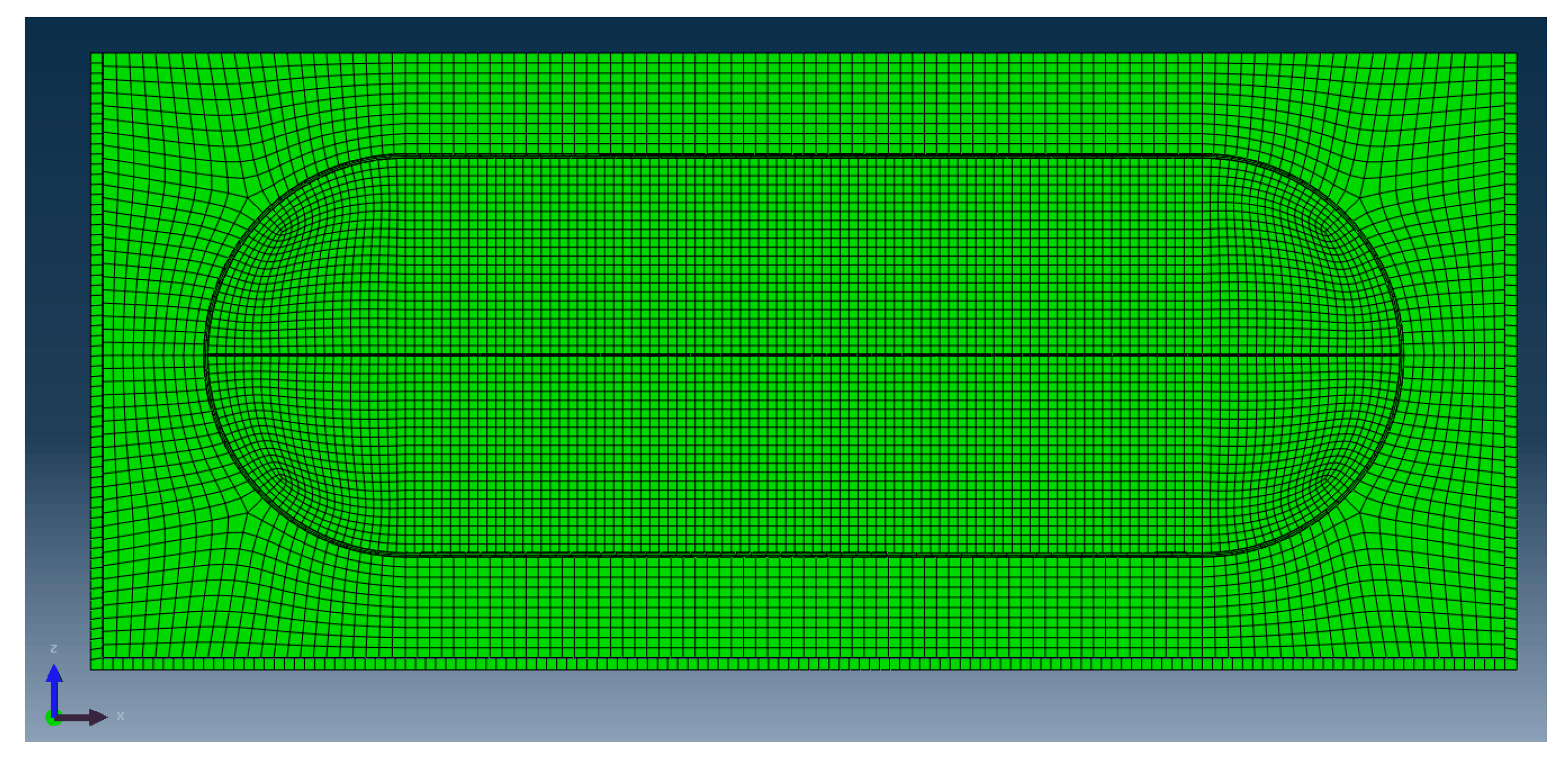
3.3. Numerical Model Description

A commercial finite element code, ABAQUS, was used to predict the BOR in the tank through a computational analysis. As the thermal conductivity model was considered, both the liquid and gas were modeled, and an extremely thin layer was implemented as the boundary layer of the gas. The effective thermal conductivity of the boundary layer, K_eff was calculated using Equation (5). Plane symmetry conditions were implemented in the model, to reduce the computation time.

PUF, with a density of 96 kg/m³, was used as the heat insulation material. The thermal conductivity of PUF according to the temperature is presented in

Table 3. Material property for thermal analysis.

Item	Temperature (K)	Thermal Conductivity (mW/m-K)	Density (kg/m3)	Specific Heat (J/kg-K)
PUF	100	0.0163	96	1500
	140	0.0212
	170	0.0246
	200	0.0266
	230	0.0248
Stainless 304L	100	9.75	7860	499
	150	11.55
	200	12.89
	250	13.9
Plywood	-	0.13	880	1260

. The physical properties for the FEA analysis are listed in

Table 4. Test results of BOR experiment.

FR (%)	Mm	Ms	BOR(%)
98	93.5	95.41	-
90	85.9		28.27
80	76.3		29.74
70	66.8		38.22
60	57.2		42.61
50	47.7		43.14
40	38.2		43.15
30	28.6		42.68
20	19.1		41.08
10	9.5		36.91

. The initial temperature was that obtained experimentally for each FR, and the natural convection condition was assigned to the outside. The BOR was predicted by calculating the aggregate heat flux flowing into the tank. The mesh convergence test was performed to determine the size of the element. The heat flux between the liquid and gas at 50% FR was compared for different mesh sizes. As shown in Figure 5, the heat flux converged for an element size of approximately 10 mm. Therefore, in the heat transfer analysis, the element type was set as DC3D8 in ABAQUS, and the generated mesh is shown in Figure 6.

4. Results and Discussion

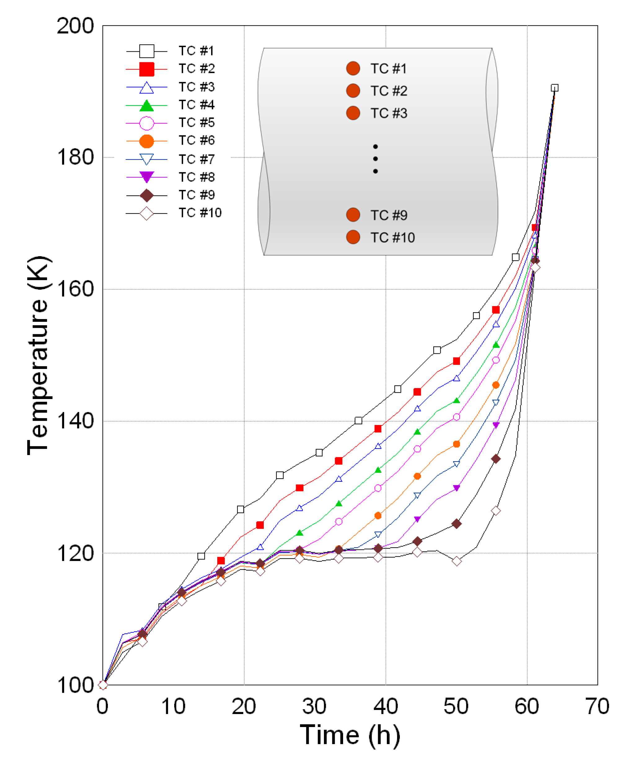
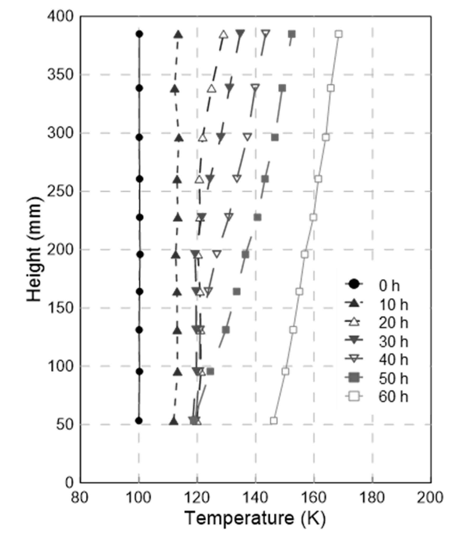
4.1. Experiment Results

As shown at Figure 7, liquid nitrogen was present at 77 K at atmospheric pressure; however, the temperature converged at 100 K owing to the increase in the saturation temperature after the pressurization process. During the initial 20 h, the pressure inside the tank increased to a set pressure of 1.5 MPa, and the temperature of the liquid increased accordingly. At this stage, because the convection of the vapor did not occur, isothermal temperature behavior was observed. Vaporized convection occurred near TC 10, corresponding to the 98% level, resulting in a rise in the temperature. Thereafter, due to the circulation caused by the temperature difference in the liquid in the upper and lower parts, the isothermal temperature distribution did not occur. In particular, the temperature variation due to the phase changes was not significant in the bounder layer, owing to the temperature distribution generated by the central jet in the stratified section. After 55 h, the temperature inside the tank rose sharply, and most of the liquid evaporated, thereby forming a pressure tank.

The initial pressurization reduced the weight loss owing to the increase in the temperature of the liquid nitrogen, thereby inhibiting the vaporization, which decreased the BOR. The WS was used to determine the difference in the BOR over time, and the changes in the mass over time were as shown in Figure 8. Except in the stages immediately after the buffering and immediately before the exhaustion, a linear behavior was observed. As time elapsed, the pressure was maintained at 1.5 MPa, and a certain amount of BOG was released. The BOR for the different mass changes was as defined in Equation (11):

$$BOR=\frac{d{M}_m/dt}{M_s}\times 24\times 100(\%)$$

(11)

where M_m is the weight of the liquid nitrogen measured in real-time, and M_s is the weight of the total liquid nitrogen.

In the context of the given period, the least count of the WS was limited; therefore, the time according to the FR for each 10% unit was set as dt, and the BOR values according to time are listed in Table 4. The BOR increased and later decreased as FR decreased, likely because of the active heat exchange with the liquids due to the augmented convection of the internal gases. As the pressure increased, the temperature of the saturated vapor increased, thereby preventing the evaporation of the liquid. Therefore, when the pressure increased after buffering, the BOR was smaller than that at the other FRs.

Figure 9 shows the temperature profile with time, for the different levels. Immediately after the liquid nitrogen buffering (0 h), the vertical temperature profile was almost identical. After 10 h, despite the formation of internal vaporization gases, the vertical temperature profile pertaining to the increase in the temperature of the liquid did not change significantly during the tank pressurization [43]. Over time, a thermal stratification region occurred at the liquid and gas boundaries, resulting in a certain temperature distribution. When half of the liquid nitrogen was exhausted at 30 h, a temperature difference occurred near the height of 200 mm, and a thermal strain was observed from the tank bottom, even though a certain amount of liquid nitrogen remained after 50 h.

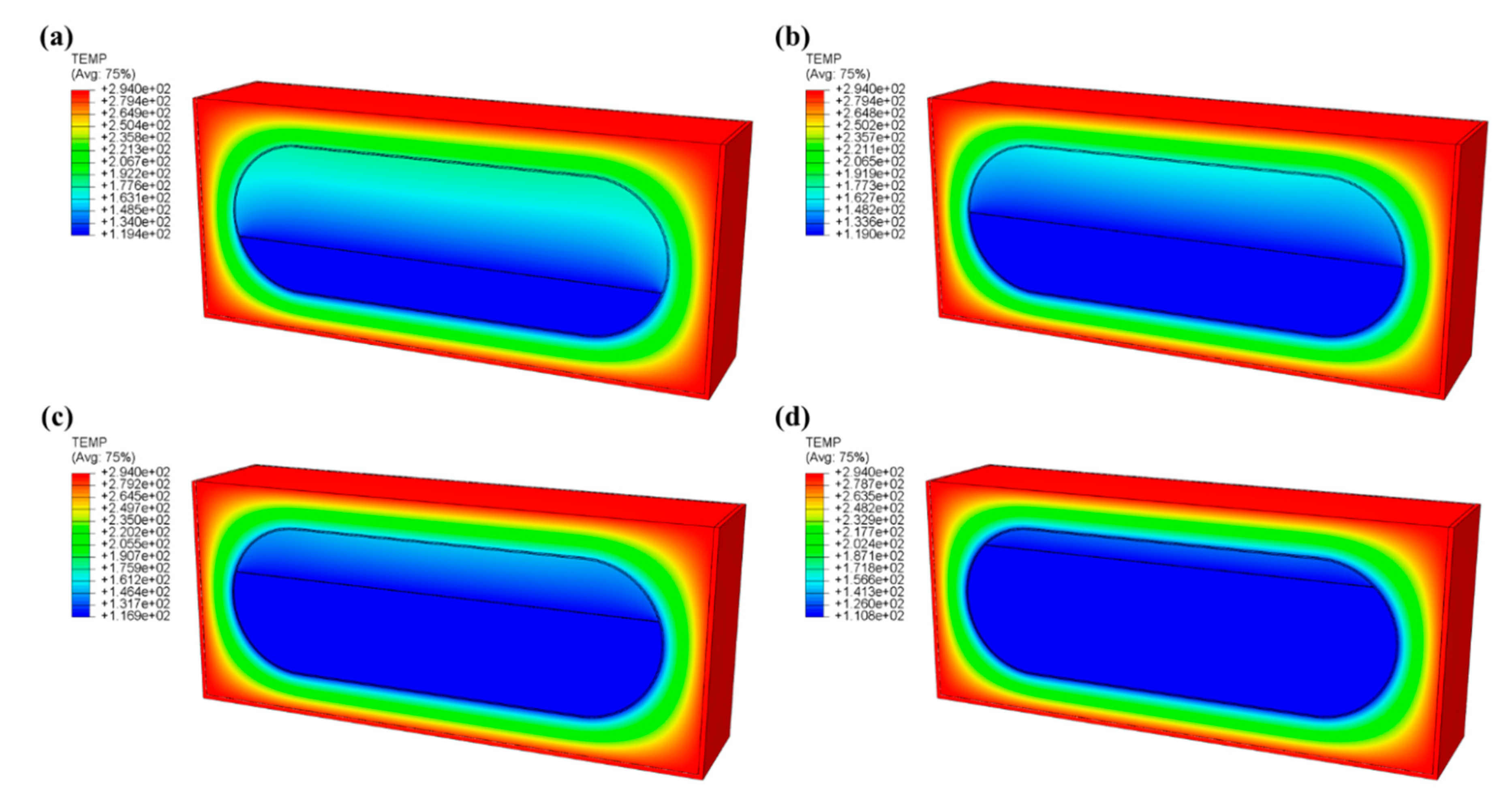
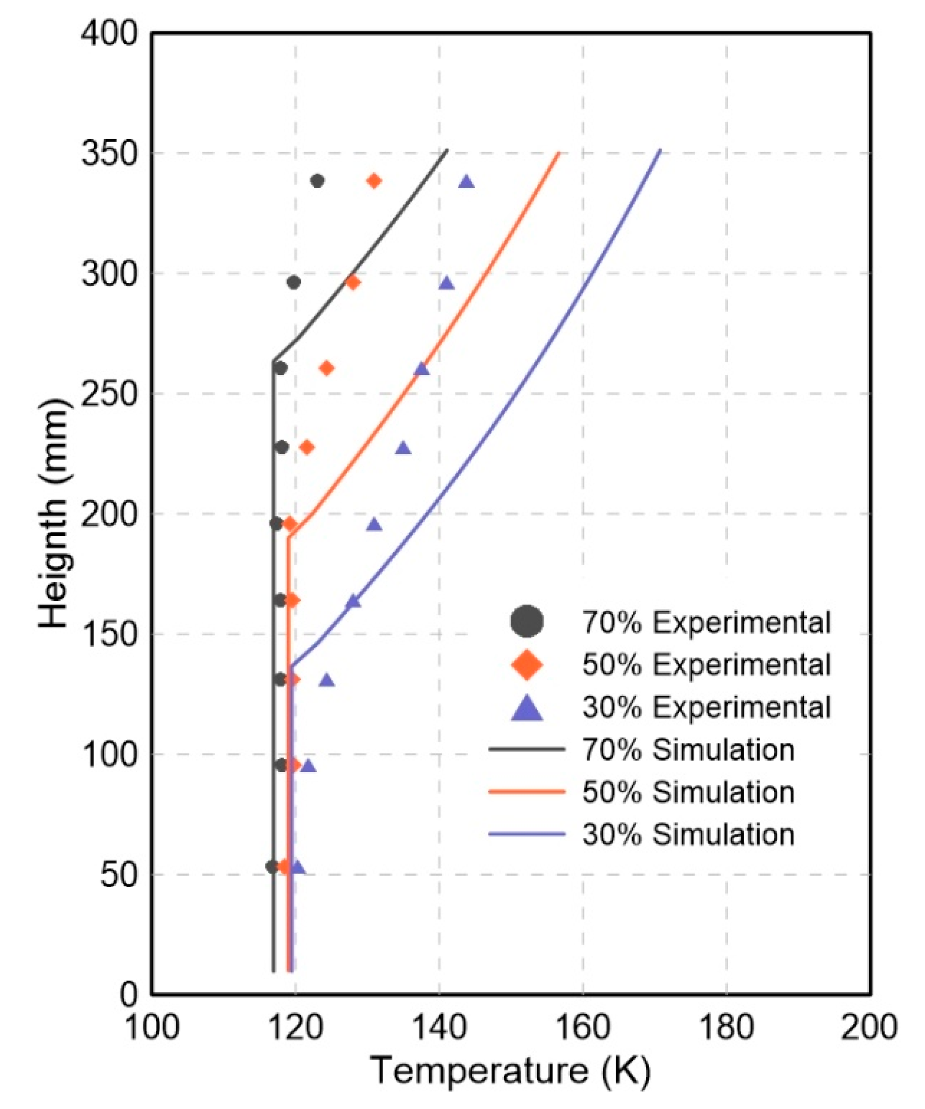
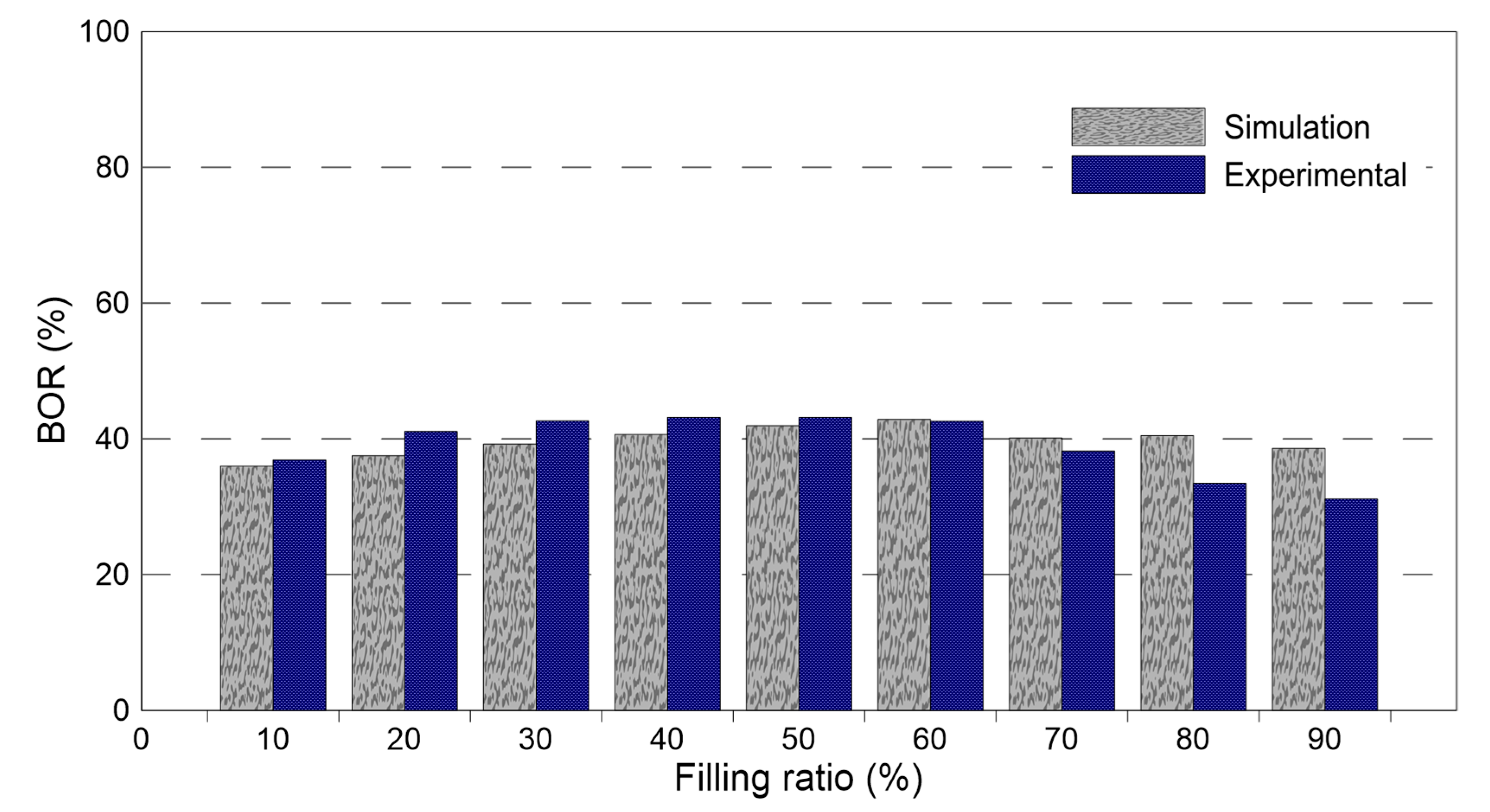
4.2. Numerical Analysis Results and Prediction of BOR

The thermal analysis of the cubic fuel tank for ships was performed using a numerical method via commercial finite element codes. The temperature of the internal liquid nitrogen was set as the initial boundary condition, as obtained experimentally. Figure 10a–d show the temperature distribution of the tank according to the numerical analysis results for each FR. As shown in Figure 10a, a large temperature gradient occurred in the vapor layer, and a temperature of 140 K was noted at the top of the tank. However, as shown in Figure 10d, the temperature gradient of the gas part was not significant, and a temperature distribution of 110 K to 130 K was observed at the top of the tank. In the insulation temperature distribution, a temperature gradient occurred along the cylindrical part of the tank. At the corners of the insulation system, the temperature was similar to the ambient temperature.

Figure 11 shows the comparison of the predicted and experimentally obtained vertical temperature profiles for each FR. The temperature gradient for the gas parts was larger than that for the liquid part, likely owing to the assumptions considered in the thermal conductivity model. Because the momentum of the gas due to the evaporation of the liquid was not considered, the temperature at the top of the tank, as obtained using the thermal conductivity model, was higher than the experimentally obtained value. This tendency was more notable at smaller FRs. Nevertheless, because the effective thermal conductivity was applied to the adjacent layers of the gas boundary to predict the BOR through FEA, a realistic heat ingress value was expected to be obtained.

The BOR was calculated by combining the heat flux from the contact surface of the tank to the gas. The BOR obtained through the simulation and experiment are shown in Figure 12. In both the settings, as the FR decreased, the BOR increased and later decreased under a certain volume. The experimental BOR was slightly lower than the simulation value for the FR ranging from 70% to 90%. As the initial design pressure was set as 1.5 MPa, the BOG was not generated immediately after the experiment commenced. The maximum error of 19% was observed at an FR of approximately 90%, likely because of the ambiguity of the buffering point in the time measurement during the experiment. As the FR decreased, K_eff increased, resulting in a higher BOR. When the FR increased to 50%, the area of contact in the liquid area reduced, and the resulting heat inflow reduced.

5. Conclusions

Experimental and numerical analyses were conducted to predict the BOR of a cubic IMO type C independent tank for small ships. In the experiment, the BOR was measured using a WS, and TCs were welded on the tank to analyze the surface temperature according to the FR. The BOR of the designed cubic tank was slightly larger than that for the LNG tank for commercial ships by approximately 35; nevertheless, this difference can likely be reduced by changing the thickness and density of the insulation material. The measured BOR using FEA is expected to have an error rate of less than 10%. The following key conclusions were derived:

(1)

In the early stage of the BOR experiment, the rise in the pressure inside the tank was dominant due to the gas generation owing to the evaporation. This phenomenon increased the saturation temperature of the liquid nitrogen, and the internal liquid temperature converged to 105 K. Therefore, under high FRs, the amount of BOG generation was the smallest.

(2)

When analyzing the finite element of the fuel tank through the thermal conductivity model, the error can be reduced by applying the effective thermal conductivity value to the boundary layer of the gas instead of considering the hydrodynamic behavior. In particular, in this work, the BOR prediction was relatively accurate during the pressure convergence period compared to that in the experiment. In this regard, it is necessary to verify the effective thermal conductivity values depending on various empirical formulas and to consider the parameters for the section in which the pressure changes.

References

1. Herdzik, J. Emissions from marine engines versus IMO certification and requirements of tier 3. J. KONES 2011, 18, 161–167. [Google Scholar]
2. Azzara, A.A.; Rutherford, D.; Wang, H. Feasibility of IMO Annex VI Tier III implementation using Selective Catalytic Reduction. Int. Counc. Clean Transp. 2014, 9, 161–167. [Google Scholar]
3. Lee, C.S.; Cho, J.R.; Kim, W.S.; Noh, B.J.; Kim, M.H.; Lee, J.M. Evaluation of sloshing resistance performance for LNG carrier insulation system based on fluid-structure interaction analysis. Int. J. Nav. Archit. Ocean Eng. 2013, 5, 1–20. [Google Scholar] [CrossRef]
4. Migliore, C.; Salehi, A.; Vesovic, V. A non-equilibrium approach to modelling the weathering of stored Liquefied Natural Gas (LNG). Energy 2017, 124, 684–692. [Google Scholar] [CrossRef]
5. Yoo, B.Y. The development and comparison of CO2 BOG re-liquefaction processes for LNG fueled CO2 carriers. Energy 2017, 127, 186–197. [Google Scholar] [CrossRef]
6. Schinas, O.; Butler, M. Feasibility and commercial considerations of LNG-fueled ships. Ocean Eng. 2016, 122, 84–96. [Google Scholar] [CrossRef]
7. Lee, H.J.; Yoo, S.H.; Huh, S.Y. Economic benefits of introducing LNG-fuelled ships for imported flour in South Korea. Transp. Res. Part D Transp. Environ. 2020, 78, 102220. [Google Scholar] [CrossRef]
8. Kwak, D.H.; Heo, J.H.; Park, S.H.; Seo, S.J.; Kim, J.K. Energy-efficient design and optimization of boil-off gas (BOG) re-liquefaction process for liquefied natural gas (LNG)-fuelled ship. Energy 2018, 148, 915–929. [Google Scholar] [CrossRef]
9. Kim, D.; Hwang, C.; Gundersen, T.; Lim, Y. Process design and economic optimization of boil-off-gas re-liquefaction systems for LNG carriers. Energy 2019, 173, 1119–1129. [Google Scholar] [CrossRef]
10. Romero Gómez, J.; Romero Gómez, M.; Lopez Bernal, J.; Baaliña Insua, A. Analysis and efficiency enhancement of a boil-off gas reliquefaction system with cascade cycle on board LNG carriers. Energy Convers. Manag. 2015, 94, 261–274. [Google Scholar] [CrossRef]
11. Krikkis, R.N. A thermodynamic and heat transfer model for LNG ageing during ship transportation. Towards an efficient boil-off gas management. Cryogenics 2018, 92, 76–83. [Google Scholar] [CrossRef]
12. Lee, J.S.; You, W.H.; Yoo, C.H.; Kim, K.S.; Kim, Y. An experimental study on fatigue performance of cryogenic metallic materials for IMO type B tank. Int. J. Nav. Archit. Ocean Eng. 2013, 5, 580–597. [Google Scholar] [CrossRef] [Green Version]
13. Kim, D.H.; Jeong, H.B.; Choi, S.H.; Jo, Y.C.; Kim, D.E.; Jeong, T. Structural assessment under sloshing impact for the IMO type b independent LNG tank. Proc. Int. Offshore Polar. Eng. Conf. 2014, 3, 180–185. [Google Scholar]
14. Kim, T.W.; Kim, S.K.; Park, S.B.; Lee, J.M. Design of Independent Type-B LNG Fuel Tank: Comparative Study between Finite Element Analysis and International Guidance. Adv. Mater. Sci. Eng. 2018, 2018. [Google Scholar] [CrossRef] [Green Version]
15. Adom, E.; Islam, S.Z.; Ji, X. Modelling of Boil-off Gas in LNG tanks: A case study. Int. J. Eng. Technol. 2010, 2, 292–296. [Google Scholar]
16. Qu, Y.; Noba, I.; Xu, X.; Privat, R.; Jaubert, J.N. A thermal and thermodynamic code for the computation of Boil-Off Gas–Industrial applications of LNG carrier. Cryogenics 2019, 99, 105–113. [Google Scholar] [CrossRef]
17. Kulitsa, M.; Wood, D.A. LNG rollover challenges and their mitigation on Floating Storage and Regasification Units: New perspectives in assessing rollover consequences. J. Loss Prev. Process Ind. 2018, 54, 352–372. [Google Scholar] [CrossRef]
18. Lee, J.-S.; Kim, K.-S.; Kim, Y. Development of an insulation performance measurement unit for full-scale LNG cargo containment system using heat flow meter method. Int. J. Nav. Archit. Ocean Eng. 2018, 10, 458–467. [Google Scholar] [CrossRef]
19. Gavelli, F.; Bullister, E.; Kytomaa, H. Application of CFD (Fluent) to LNG spills into geometrically complex environments. J. Hazard. Mater. 2008, 159, 158–168. [Google Scholar] [CrossRef]
20. Zakaria, M.S.; Osman, K.; Saadun, M.N.A.; Manaf, M.Z.A.; Mohd Hanafi, M.H. Computational simulation of boil-off gas formation inside liquefied natural gas tank using evaporation model in ANSYS fluent. Appl. Mech. Mater. 2013, 393, 839–844. [Google Scholar] [CrossRef]
21. Saleem, A.; Farooq, S.; Karimi, I.A.; Banerjee, R. A CFD simulation study of boiling mechanism and BOG generation in a full-scale LNG storage tank. Comput. Chem. Eng. 2018, 115, 112–120. [Google Scholar] [CrossRef]
22. Lee, J.H.; Kim, Y.J.; Hwang, S. Computational study of LNG evaporation and heat diffusion through a LNG cargo tank membrane. Ocean Eng. 2015, 106, 77–86. [Google Scholar] [CrossRef]
23. Ovidi, F.; Pagni, E.; Landucci, G.; Galletti, C. Numerical study of pressure build-up in vertical tanks for cryogenic flammables storage. Appl. Therm. Eng. 2019, 161, 114079. [Google Scholar] [CrossRef]
24. Scurlock, R.G. Stratification, Rollover and Handling of LNG, LPG and Other Cryogenic Liquid Mixtures; Springer: Berlin/Heidelberg, Germany, 2015. [Google Scholar]
25. Kang, M.; Kim, J.; You, H.; Chang, D. Experimental investigation of thermal stratification in cryogenic tanks. Exp. Therm. Fluid Sci. 2018, 96, 371–382. [Google Scholar] [CrossRef]
26. Lin, Y.; Ye, C.; Yu, Y.-y.; Bi, S.-w. An approach to estimating the boil-off rate of LNG in type C independent tank for floating storage and regasification unit under different filling ratio. Appl. Therm. Eng. 2018, 135, 463–471. [Google Scholar] [CrossRef]
27. Tsili, M.A.; Amoiralis, E.I.; Kladas, A.G.; Souflaris, A.T. Power transformer thermal analysis by using an advanced coupled 3D heat transfer and fluid flow FEM model. Int. J. Therm. Sci. 2012, 53, 188–201. [Google Scholar] [CrossRef]
28. Shen, Y.; Zhang, B.; Xin, D.; Yang, D.; Peng, X. 3-D finite element simulation of the cylinder temperature distribution in boil-off gas (BOG) compressors. Int. J. Heat Mass Transf. 2012, 55, 7278–7286. [Google Scholar] [CrossRef]
29. Mohanraj, M.; Jayaraj, S.; Muraleedharan, C. Applications of artificial neural networks for thermal analysis of heat exchangers–a review. Int. J. Therm. Sci. 2015, 90, 150–172. [Google Scholar] [CrossRef]
30. Giannett, N.; Redo, M.A.; Jeong, J.; Yamaguchi, S.; Saito, K.; Kim, H. Prediction of two-phase flow distribution in microchannel heat exchangers using artificial neural network. Int. J. Refri. 2020, 111, 53–62. [Google Scholar] [CrossRef]
31. Kim, J.H.; Park, W.S.; Chun, M.S.; Kim, J.J.; Bae, J.H.; Kim, M.H.; Lee, J.M. Effect of pre-straining on low-temperature mechanical behavior of AISI 304L. Mater. Sci. Eng. A 2012, 543, 50–57. [Google Scholar] [CrossRef]
32. Convention, I. 1983 Amendments to the International Convention for the Safety of Life International Code for the Construction and Equipment of Ships Carrying Liquefied Gases in Bulk; (IGC Code) International Code for the Construction and Equipment of Ships Carrying Liq: London, UK, 1998; p. 15. [Google Scholar]
33. Lee, J.; Choi, Y.; Jo, C.; Chang, D. Design of a prismatic pressure vessel: An engineering solution for non-stiffened-type vessels. Ocean Eng. 2017, 142, 639–649. [Google Scholar] [CrossRef]
34. Park, S.B.; Lee, C.S.; Choi, S.W.; Kim, J.H.; Bang, C.S.; Lee, J.M. Polymeric foams for cryogenic temperature application: Temperature range for non-recovery and brittle-fracture of microstructure. Compos. Struct. 2016, 136, 258–269. [Google Scholar] [CrossRef]
35. Kim, J.H.; Choi, S.W.; Park, D.H.; Park, S.B.; Kim, S.K.; Park, K.J.; Lee, J.M. Effects of cryogenic temperature on the mechanical and failure characteristics of melamine-urea-formaldehyde adhesive plywood. Cryogenics 2018, 91, 36–46. [Google Scholar] [CrossRef]
36. Ma, H.; Cai, W.; Zheng, W.; Chen, J.; Yao, Y.; Jiang, Y. Stress characteristics of plate-fin structures in the cool-down process of LNG heat exchanger. J. Nat. Gas Sci. Eng. 2014, 21, 1113–1126. [Google Scholar] [CrossRef]
37. Li, X.; Xie, G.; Wang, R. Experimental and numerical investigations of fluid flow and heat transfer in a cryogenic tank at loss of vacuum. Heat Mass Transf. Und. Stoffuebertragung 2010, 46, 395–404. [Google Scholar] [CrossRef]
38. Woodfield, P.L.; Monde, M.; Mitsutake, Y. Measurement of Averaged Heat Transfer Coefficients in High-Pressure Vessel during Charging with Hydrogen, Nitrogen or Argon Gas. J. Therm. Sci. Technol. 2007, 2, 180–191. [Google Scholar] [CrossRef] [Green Version]
39. Joseph, J.; Agrawal, G.; Agarwal, D.K.; Pisharady, J.C.; Sunil Kumar, S. Effect of insulation thickness on pressure evolution and thermal stratification in a cryogenic tank. Appl. Therm. Eng. 2017, 111, 1629–1639. [Google Scholar] [CrossRef]
40. Bashiri, A.; Fatehnejad, L. Modeling and simulation of rollover in LNG storage tanks. Int. Gas Union World Gas Conf. Pap. 2006, 5, 2522–2528. [Google Scholar]
41. Jazayeri, S.A.; Khoei, E.M.H. Numerical comparison of thermal stratification due natural convection in densified LOX and LN2 tanks. Am. J. Appl. Sci. 2008, 5, 1773–1779. [Google Scholar] [CrossRef] [Green Version]
42. Ludwig, C.; Dreyer, M.E.; Hopfinger, E.J. Pressure variations in a cryogenic liquid storage tank subjected to periodic excitations. Int. J. Heat Mass Transf. 2013, 66, 223–234. [Google Scholar] [CrossRef]
43. Seo, M.; Jeong, S. Analysis of self-pressurization phenomenon of cryogenic fluid storage tank with thermal diffusion model. Cryogenics 2010, 50, 549–555. [Google Scholar] [CrossRef]
Figure 1. Schematic of experiment and arrangement for TC.
Jmse 09 00036 g001
Figure 2. Data acquisition apparatus to measure inner tank surface temperature (a) Spot welding of thermal couple (b) data acquisition system
Jmse 09 00036 g002
Figure 3. Schematic diagram of (a) heat transfer model, (b) hydrodynamic model.
Jmse 09 00036 g003
Figure 4. Flow chart depicting solution procedure.
Jmse 09 00036 g004
Figure 5. Results of mesh convergence test.
Jmse 09 00036 g005
Figure 6. Elements of analysis model.
Jmse 09 00036 g006
Figure 7. Time dependent temperature distributions of inner tank at each point.
Jmse 09 00036 g007
Figure 8. Time dependent liquid nitrogen weight.
Jmse 09 00036 g008
Figure 9. Vertical temperature profile over time.
Jmse 09 00036 g009
Figure 10. Temperature distributions of analysis model at each FR (a) 30% (b) 50% (c) 70% (d) 90%.
Jmse 09 00036 g010
Figure 11. Comparison between experiments and numerical analysis for vertical temperature profile.
Jmse 09 00036 g011
Figure 12. Comparison of BOR with simulation and experimental.
Jmse 09 00036 g012