1. Introduction
During the past few decades, the interest in underwater intervention has grown exponentially as more often it is necessary to perform underwater tasks like surveying, sampling, archaeology exploration or industrial infrastructure inspection and maintenance of offshore oil and gas structures, submerged oil wells or pipeline networks, among others [
1,
2,
3,
4,
5].
Historically, scuba diving has been the prevailing method of conducting the aforementioned tasks. However, performing these missions in a harsh environment like open water scenarios is slow, dangerous, and resource consuming. More recently, thanks to technological advances such as Remotely Operated Vehicles (ROVs) equipped with manipulators, more deep and complex underwater scenarios are accessible for scientific and industrial activities.
Nonetheless, these
ROVs have complex dynamics that make their piloting a difficult and error-prone task, requiring trained operators. In addition, these vehicles require a support vessel, which leads to expensive operational costs. To mitigate that, some research centres have started working towards intervention Autonomous Underwater Vehicles (
AUVs) [
6,
7,
8]. In addition, due to the complexity of the Underwater Vehicle Manipulator Systems (UVMS), recent studies have been published towards its control [
9,
10].
Traditionally, when operating in unknown underwater environments, acoustic bathymetric maps are used to get a first identification of the environment. Once the bathymetric information is available,
ROVs or
AUVs can be sent to obtain more detailed information using short distance sensors with higher resolution. The two main perception modalities used at close range are laser and video, thanks to their high resolution. They are used during the approach, object recognition and intervention phases. Existing solutions for all perception modalities are reviewed in
Section 2.1.
The underwater environment is one of the most problematic in terms of sensing in general and in terms of object perception in particular. The main challenges of underwater perception include distortion in signals, light propagation artefacts like absorption and scattering, water turbidity changes or depth-depending colour distortion.
Accurate and robust object detection, identification of target objects in different experimental conditions and pose estimation are essential requirements for the execution of manipulation tasks.
In this work, we propose a deep learning based approach to recognise pipes and valves in multiple underwater scenarios, using the 3D RGB point cloud information provided by a stereo camera, for real-time AUV inspection and manipulation tasks.
The remainder of this paper is structured as follows:
Section 2 reviews related work on underwater perception and pipe and valve identification and highlights the main contributions of this work.
Section 3 describes the adopted methodology and materials used in this study. The experimental results are presented and discussed in
Section 4. Finally,
Section 5 outlines the main conclusions and future work.
2. Related Work and Contributions
2.1. State of the Art
Even though computer vision is one of the most complete and used perception modalities in robotics and object recognition tasks, it has not been widely used in underwater scenarios. Light transmission problems and water turbidity affect the images clarity, colouring and produce distortions; these factors have favoured the usage of other perception techniques.
Sonar sensing has been largely used for object localisation or environment identification in underwater scenarios [
11,
12]. In [
13], Kim et al. present an AdaBoost based method for underwater object detection, while Wang et al. [
14] propose a combination of non-local spatial information and frog leaping algorithm to detect underwater objects in sonar images. More recently, object detection deep learning techniques have started to apply over sonar imaging in applications such as detection of underwater bodies in [
15,
16] or underwater mine detection in [
17]. Sonar imaging also presents some drawbacks as it tends to generate noisy images, losing texture information; and are not capable of gathering colour information, which is useful in object recognition tasks.
Underwater laser scans are another perception technique used for object recognition, providing accurate 3D data. In [
18], Palomer et al. present the calibration and integration of a laser scanner on an AUV for object manipulation. Himri et al. [
19,
20] use the same system to detect objects using a recognition and pose estimation pipeline based on point cloud matching. Inzartsev et al. [
21] simulate the use of a single beam laser paired with a camera to capture its deformation and track an underwater pipeline. Laser scans are also affected by light transmission problems, have a very high initial cost and can only provide colourless point clouds.
The only perception modality that allows gathering of colour information for the scene is computer vision. Furthermore, some of its aforementioned weaknesses can be mitigated by adapting to the environmental conditions, adjusting the operation range, calibrating the cameras or colour correcting the obtained images.
Traditional computer vision approaches have been used to detect and track submerged artifacts [
22,
23,
24,
25], cables [
26,
27,
28] and even pipelines [
28,
29,
30,
31]. Some works are based on shape and texture descriptors [
28,
31] or template matching [
32,
33], while others exploit colour segmentation to find regions of interest in the images, which are later further processed [
25,
34].
On pipeline detection, Kallasi et al. in [
35] and Razzini et al. in [
7,
36] present traditional computer vision methods combining shape and colouring information to detect pipes in underwater scenarios and later project them into point clouds obtained from stereo vision. In these works, the point cloud information is not used to assist the pipe recognition process.
The first found trainable system to detect pipelines is presented in [
37] by Rekik et al. using the objects structure and content features along a Support Vector Machine to classify between positive and negative underwater pipe images samples. Later, Nunes et. al introduced the application of a Convolutional Neural Network in [
38] to classify up to five underwater objects, including a pipeline. In both of these works, no position of the object is given, but simply a binary output on the object’s presence.
The application of computer vision approaches based on deep learning in underwater scenarios has been limited to the detection and pose estimation of 3D-printed objects in [
39] or for living organisms detection like fishes [
40] or jellyfishes [
41]. Few research studies involving pipelines are restricted to damage evaluation [
42,
43] or valve detection for navigation [
44] working with images taken from inside the pipelines. The only known work addressing pipeline recognition using deep learning is from Guerra et al. in [
45], where a camera-equipped drone is used to detect pipelines in industrial environments.
To the best knowledge of the authors, there are not works applying deep learning techniques in underwater computer vision pipeline and valve recognition, nor implementing the usage of point cloud information on the detection process itself.
2.2. Main Contributions
The main contributions of this paper are composed of:
Generation of a novel point cloud dataset containing pipes and different types of valves in varied underwater scenarios, providing enough data to perform a robust training and testing of the selected deep neural network.
Implementation and testing of the PointNet architecture in underwater environments to detect pipes and valves.
Studying the suitability of the PointNet network on real-time autonomous underwater recognition tasks in terms of detection performance and inference time by tuning diverse hyperparameter values.
The datasets (point clouds and corresponding ground truths) along with a trained model are provided to the scientific community.
3. Materials and Methods
This section presents an overview of the selected network; explains the acquisition, labelling and organisation of the data; and details the studied network hyperparameters, the validation process and the evaluation metrics.
3.1. Deep Learning Network
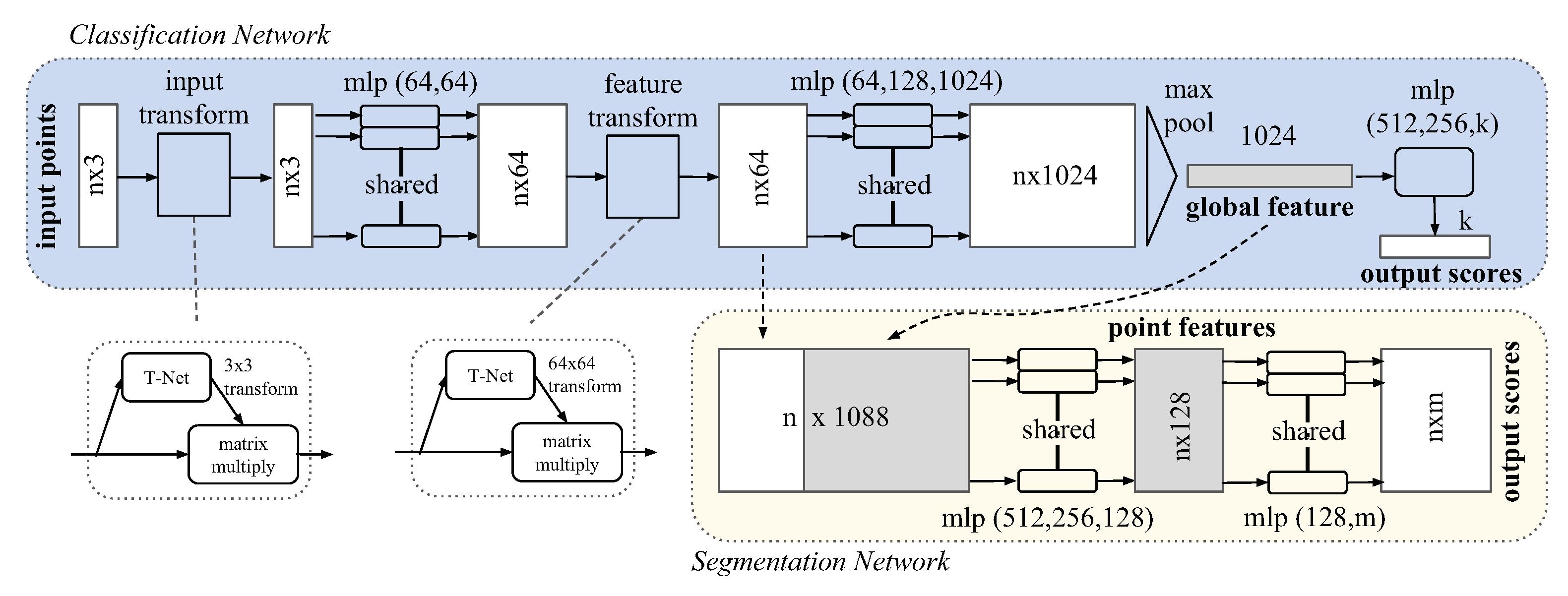
To perform the pipe and valve 3D recognition from point cloud segmentation, we selected the PointNet deep neural network [
46]. This is a unified architecture for applications ranging from object classification and part segmentation to scene semantic segmentation. PointNet is a highly efficient and effective network, obtaining great metrics in both object classification and segmentation tasks in indoor and outdoor scenarios [
46]. However, it has never been tested in underwater scenarios. The whole PointNet architecture is shown in
Figure 1.
In this paper, we use the
Segmentation Network of PointNet. This network is an extension to the
Classification Network, as it can be seen in
Figure 1. Some of its key features include:
The integration of max pooling layers as symmetric function to aggregate the information from each point, making the model invariant to input permutations.
Being able to predict per point features that rely both on local structures from nearby points and global information which makes the prediction invariant to object transformations such as translations or rotations. This combination of local and global information is obtained by concatenating the global point cloud feature vector with the local per point features.
Making the semantic labeling of a point cloud invariant to the point cloud geometric transformations by aligning all input set to a canonical space before feature extraction. To achieve this, an affine transformation matrix is predicted using a mini-network (T-net in
Figure 1) and directly applied to the coordinates of input points.
The PointNet architecture takes as input point clouds and it outputs a class label for each point. During the training, the network is also fed with ground truth point clouds, where each point is labelled with its pertaining class. The labelling process is further detailed in
Section 3.2.2.
As the original PointNet implementation, we used a softmax cross-entropy loss along an Adam optimiser. The decay rate for batch normalisation starts with 0.5 and is gradually increased to 0.99. In addition, we applied a dropout with keep ratio 0.7 on the last fully connected layer, before class score prediction. Other hyperparameters values such as learning rate or batch size are discussed, along other parameters, on
Section 3.3.
Furthermore, to improve the network performance, we implemented an early stopping strategy based on the work of Prechelt in [
47], assuring that the network training process stops at an epoch that ensures minimum divergence between validation and training losses. This technique allows for obtaining a more general and broad training, avoiding overfitting.
3.2. Data
This subsection explains the acquisition, labelling and organisation of the data used to train and test the PointNet neural network.
3.2.1. Acquisition
As mentioned in
Section 3.1, the PointNet uses pointclouds for its training and inference. To obtain the point clouds, we set up a Bumblebee2 Firewire stereo rig [
48] on an Autonomous Surface Vehicle (ASV) through a
Robot Operating System (ROS) framework.
First, we calibrated the stereo rig both on fresh and salt water using the ROS package
image_pipeline/camera_calibration [
49,
50]. It uses a chessboard pattern to obtain the camera, rectification and projection matrices along the distortion coefficients for both cameras.
The acquired synchronised pairs of left-right images (resolution: 1024 × 768 pixels) are processed as follows by the
image_pipeline/stere_image_proc ROS package [
51] to calculate the disparity between pairs of images based on epipolar matching [
52], obtaining the corresponding depth of each pixel from the stereo rig.
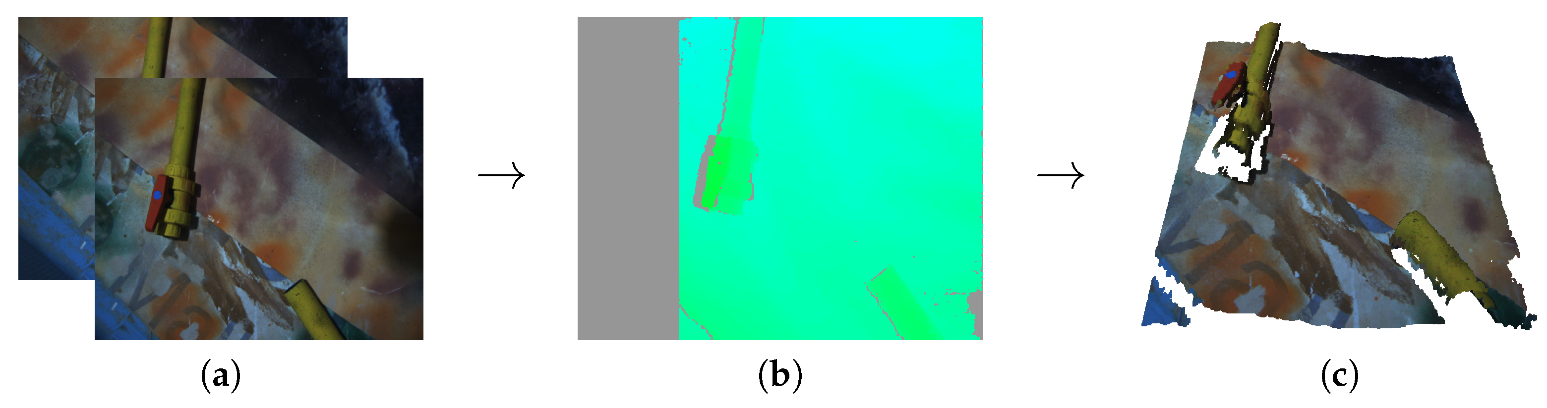
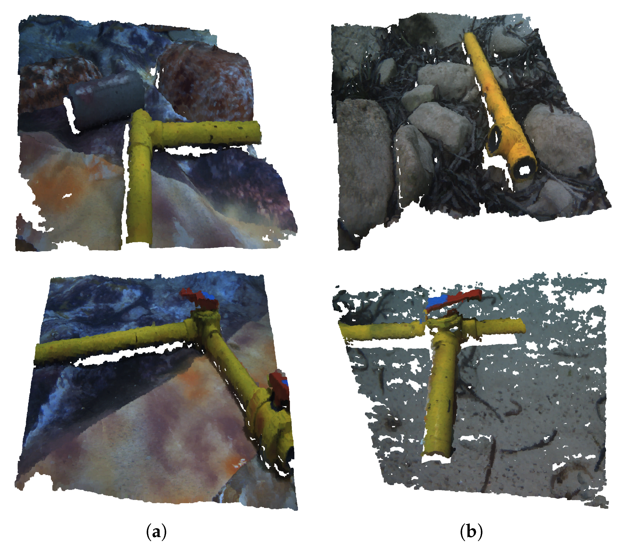
Finally, combining this depth information with the RGB colouring from the original images, we generate the point clouds. An example of the acquisition is pictured in
Figure 2.
3.2.2. Ground Truth Labelling
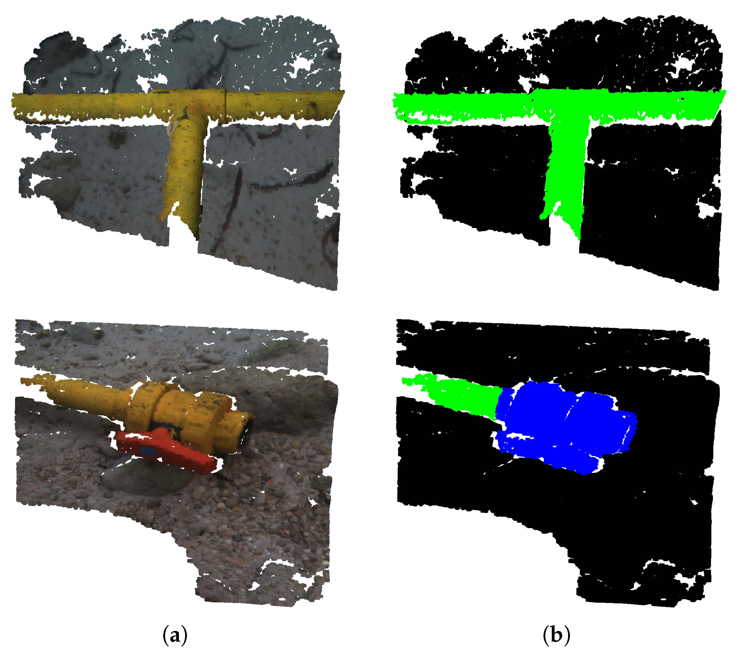
Ground truth annotations are manually built from the point clouds, where the pixels corresponding to each class are marked with a different label. The studied classes and their RGB labels are:
Pipe (0, 255, 0),
Valve (0, 0, 255) and
Background (0, 0, 0).
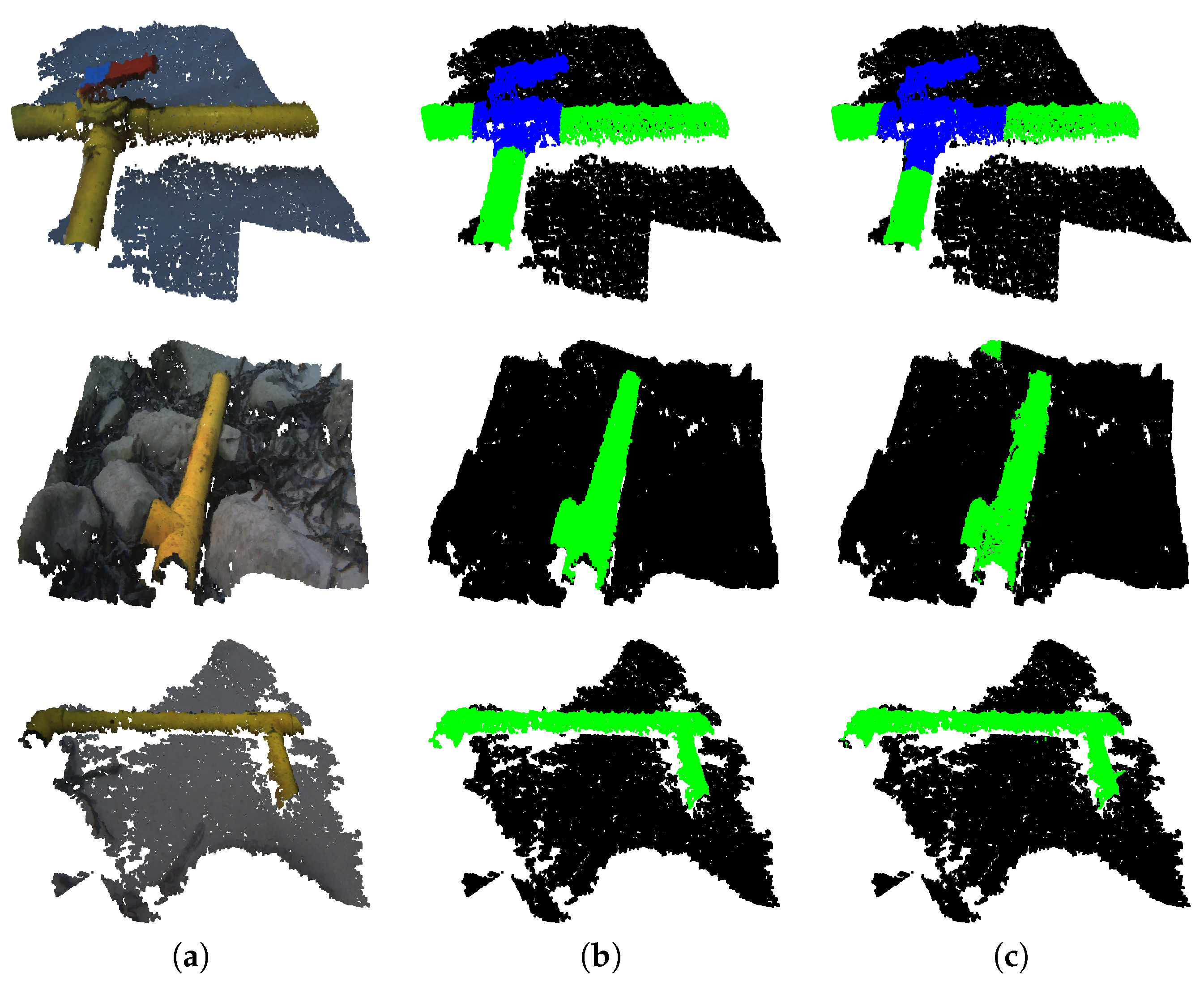
Figure 3 shows a couple of point clouds along with their corresponding ground truth annotations.
3.2.3. Dataset Managing
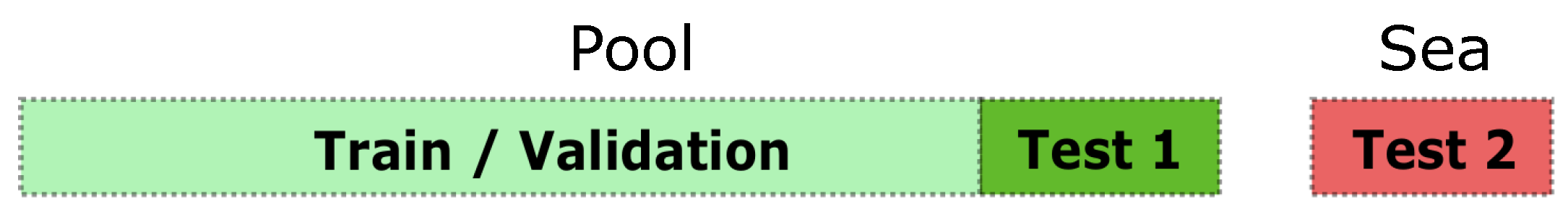
Following the steps described in the previous section, we generated two datasets. The first one includes a total of 262 point clouds along with their ground truths. It was obtained on an artificial pool and contains diverse connections between pipes of different diameters and 2/3 way valves. It also contains other objects such as cement blocks and ceramic vessels, always over a plastic sheeting simulating different textures. This dataset is split into a train-validation set (90% of the data, 236 point clouds) and a test set (10% of the data, 26 point clouds). The different combinations of elements and textures increase its diversity, helping to assure the robustness in the training and reduce overfitting. From now on, we will refer to this dataset as the Pool dataset.
The second dataset includes a total of 22 point clouds and their corresponding ground truths. It was obtained in the sea and contains different pipe connections and valves positions. In addition, these 22 point clouds were obtained over diverse types of seabed, such as sand, rocks, algae, or a combination of them. This dataset is used to perform a secondary test, as it contains point clouds with different characteristics of the ones used to train and validate the network, allowing us to assess how well the network generalises its training to new conditions. From now on, we will refer to this dataset as the Sea dataset.
Figure 4 illustrates the dataset managing, while in
Figure 5 some examples of point clouds from both datasets are shown.
3.3. Hyperparameter Study
When training a neural network, there are hyperparameters which can be tuned, changing some of the features of the network or the training process itself. We selected some of these hyperparameters and trained the network using different values to study their effect over its performance in underwater scenarios. The considered hyperparameters were:
Batch size: number of training samples utilised in one iteration before backpropagating.
Learning rate: affects the size of the matrix changes that the network takes when searching for an optimal solution.
Block (B) and stride (S) size: to prepare the network input, the point clouds are sampled into blocks of meters, with a sliding window of stride S meters.
Number of points: maximum number of allowed points per block. If it exceeds, random points are deleted. Used to control the point cloud density.
The tested values for each hyperparameter are shown in
Table 1. In total, 13 experiments are conducted, one using the hyperparameter values used in the original PointNet implementation [
46] (marked in bold in
Table 1); and 12 more, each one fixing three of the aforementioned hyperparameters to their original values and using one of the other tested values for the fourth hyperparameter. This way, the effect of each hyperparameter and its value over the performance is isolated.
3.4. Validation
3.4.1. Validation Process
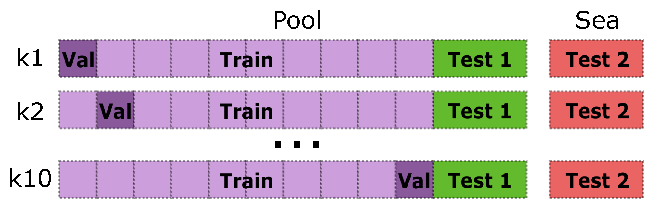
To ensure the robustness of the results generated for the 13 experiments, we used the 10 k-fold cross-validation method [
53]. Using this method, the train-validation set of the
Pool dataset is split into ten equally sized subsets. The network is trained ten times as follows, each one using a different subset as validation (23 point clouds) and the nine remaining as training (213 point clouds), generating ten models which are tested against both
Pool and
Sea test sets. Finally, each experiment performance is computed as the mean of the results of its 10 cross-validation models. This method reduces the variability of the results, as these are less dependent on the selected training and validation subsets, therefore obtaining a more accurate performance estimation.
Figure 6 depicts the k-fold cross-validation technique applied to the dataset managing described in
Section 3.2.3.
3.4.2. Evaluation Metrics
To evaluate a model performance, we make a point-wise comparison between its predictions and their corresponding ground truth annotations, generating a multi-class confusion matrix. This confusion matrix indicates, for each class: the number of points correctly identified belonging to that class,
True Positives (TP) and not belonging to it,
True Negatives (TN); the number of points misclassified as the studied class,
False Positives (FP); and the number of points belonging to that class misclassified as another one,
False Negatives (FN). Finally, the TP, FP and FN values are used to calculate the
Precision,
Recall and
F1-score for each class, following Equations (
1)–(
3):
Additionally, the mean time that a model takes to perform the inference of a point cloud is calculated. This metric is very important, as it defines the frequency that information is provided to the system. In underwater applications, it would directly affect the agility and responsiveness of the AUV that this network could be integrated in, having an impact over the final operation time.
4. Experimental Results and Discussion
This section reports the performance obtained for each experiment over the
Pool and
Sea test sets and discusses the effect of each hyperparameter over it. The notation used to name each experiment corresponds as follows: “Base” for the experiment conducted using the original hyperparameter values, marked in bold in
Table 1; the other experiments are notated as an abbreviation of the modified hyperparameter for that experiment (“Batch” for batch size, “Lr” for learning rate, “BS” for block-stride and “Np” for number of points) followed by the actual value of the hyperparameter for that experiment. For instance, experiment
Batch 24 uses all original hyperparameter values except for the batch size, which in this case is 24.
4.1. Pool Dataset Results
Table 2 shows the
F1-scores obtained for the studied classes and its mean for all experiments when evaluated over the
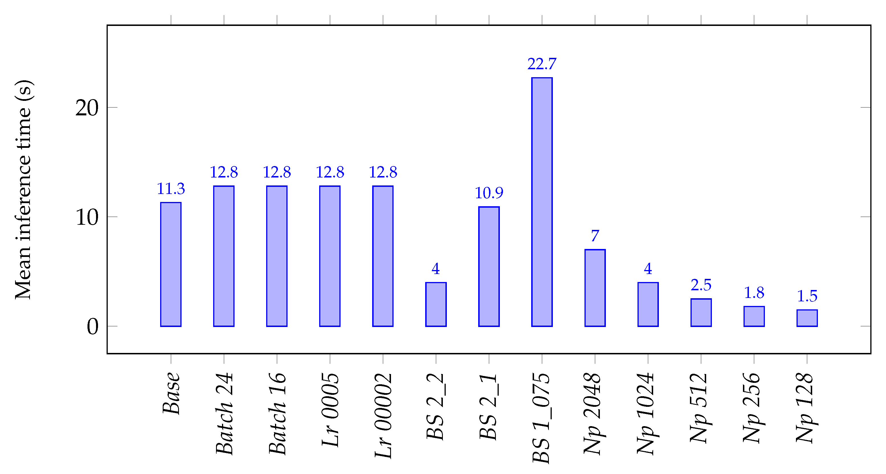
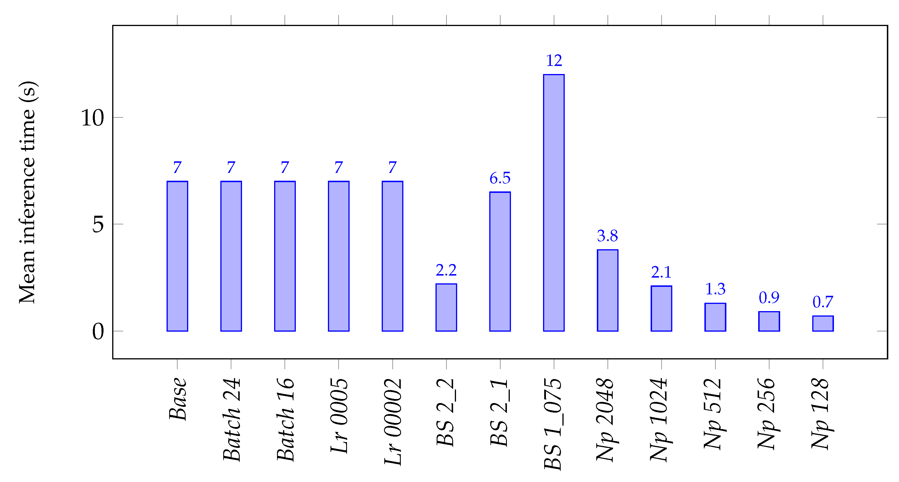
Pool test set. The mean inference time for each experiment is showcased in
Figure 7 as follows.
The results presented in
Table 2 show that all experiments achieved a mean
F1-score greater than 95.5%, with the highest value of 97.2% for the experiment
BS 1_075, which has a smaller block stride than its size, overlapping information. Considering the figures of mean
F1-score for all experiments, it is safe to say that no hyperparameter seemed to represent a major shift in the network behaviour.
Looking at the metrics presented by the best performing experiment for each class, it can be seen that the
Pipe class achieved an
F1-score of 97.1%, outperforming other state-of-the-art methods for underwater pipe segmentation: [
35]—traditional computer vision algorithms over 2D underwater images achieving an
F1-score of 94.1%, [
7]—traditional computer vision algorithms over 2D underwater images achieving a mean
F1-score over three datasets of 88.0% and [
45]—deep leaning approach for 2D drone imagery achieving a pixel-wise accuracy of 73.1%. For the valve class, the
BS 1_075 experiment achieved a
F1-score of 94.9%, being a more challenging class due to its complex geometry. As far as the authors know, no comparable work on underwater valve detection has been identified. Finally, for the more prevailing
Background class, the best performing experiment achieved an
F1-score of 99.7%.
The results on mean inference time for each experiment presented in
Figure 7 shows that the batch size and learning rate hyperparameter values do not influence the inference time or have little impact, as their value is very similar to the one obtained in the
Base experiment. On the contrary, the block and stride size highly affect the inference time, the bigger the information block or the stride between blocks, the faster the network can analyse a point cloud, and vice versa. Finally, the maximum number of allowed points per block also has a direct impact over the inference time, the lower it is, the faster the network can analyse a point cloud, as it becomes less dense. The time analysis was carried out in a computer with the following specs—processor: Intel i7-7700, RAM: 16 GB, GPU: NVIDIA GeForce GTX 1080.
Taking into account both metrics, BS 1_075 presented the best F1-score and has the highest inference time. In this experiment, the network uses a small block size and stride, being able to analyse the data and extract its features better, at the cost of taking longer. The hyperparameter values of this experiment are a good fit for a system in which quick responsiveness to changes and high frequency of information are not a priority, allowing for maximising the recognition performance.
On the other hand, experiments such as BS 2_2 or Np 1024, 512, 256, 128 were able to maintain very high F1-scores while significantly reducing the inference time. The hyperparameter values tested in these experiments are a good fit for more agile systems that need a higher frequency of information and responsiveness to changes.
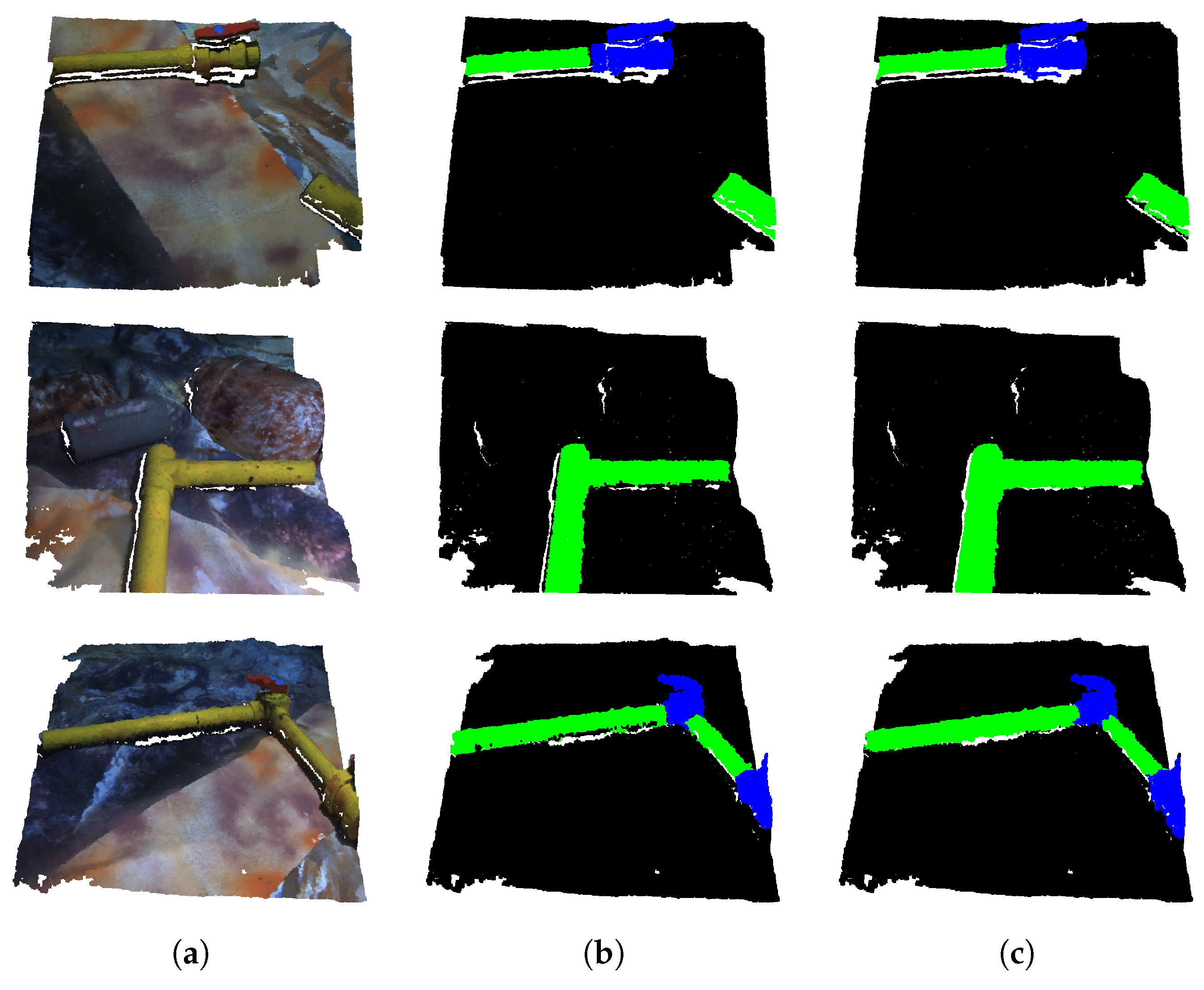
Figure 8 shows some examples of original point clouds from the
Pool test set along with their corresponding ground truth annotations and network predictions.
4.2. Sea Dataset Results
Table 3 shows the
F1-scores obtained for the studied classes and its mean, for all experiments when evaluated over the
Sea test set. The mean inference time for each experiment is showcased in
Figure 9 as follows.
The results presented in
Table 3 show that all experiments achieved a mean
F1-score greater than 84.9% with the highest value of 89.3% for the experiment
Batch 16. On average, the mean
F1-score was around 9% lower than for the
Pool test set. Even so, all experiments maintained high
F1-scores. Again, the
F1-scores of the
Pipe and
Valve classes are relatively lower than for the
Background class. Even though the
Sea test set is more challenging, as it contains unseen pipe and valve connections and environment conditions, the network was able to generalise its training and avoid overfitting.
The results on mean inference time for each experiment presented in
Figure 9 shows that the mean inference times for the
Sea test set are proportionally lower than the
Pool test set for all experiments. This occurs because the
Sea test set contains smaller point clouds with fewer points.
Figure 10 shows some examples of original point clouds from the
Sea test set along with their corresponding ground truth annotations and network predictions.
5. Conclusions and Future Work
This work studied the implementation of the PointNet deep neural network in underwater scenarios to recognise pipes and valves from point clouds. First, two datasets of point clouds were gathered, providing enough data for the training and testing of the network. From these, a train-validation set and two test sets were generated, a primary test set with similar characteristics as the training data and a secondary one containing unseen pipe and valve links and environment conditions to test the network training generalisation and overfitting. Then, diverse hyperparameter values were tested to study their effect over the network performance, both in the recognition task and inference time.
Results from the recognition task concluded that the network was able to identify pipes and valves with high accuracy for all experiments in both Pool and Sea test sets, reaching F1-scores of 97.2% and 89.3%, respectively. Regarding the network inference time, results showed that it is highly dependent on the size of information block and its stride; and to the point clouds density.
From the performed experiments, we obtained a range of models covering different trade-offs between detection performance and inference time, enabling the network implementation into a wider spectrum of systems, adapting to its detection and computational cost requirements. The BS 1_075 experiment presented metrics that fitted a slower, more still system, while experiments like BS 2_2 or Np 1024, 512, 256, 128 are a good fit for more agile and dynamic systems.
The implementation of the PointNet network in underwater scenarios presented some challenges, like ensuring its recognition performance when trained with point clouds obtained from underwater images, and its suitability to be integrated on an AUV due to its computational cost. With the results obtained in this work, we have demonstrated the validity of the PointNet deep neural network to detect pipes and valves in underwater scenarios for AUV manipulation and inspection tasks.
The datasets and code, along with one of the
Base experiment trained models, are publicly available at
http://srv.uib.es/3d-pipes-1/ (UIB-SRV-3D-pipes) for the scientific community to test or replicate our experiments.
Further steps need to be taken in order to achieve an underwater object localisation and positioning for ROV and AUV intervention using the object recognition presented in this work. We propose the following future work:
Performing an instance-based detection from the presented pixel-based one, allowing for recognition of pipes and valves as a whole object and to classify them by type (two or three way) or status (opened or closed).
Using the depth information provided by the stereo cameras along with the instance detection to achieve a spatial 3D positioning of each object. Once the network is implemented in an AUV, this would provide the vehicle with the information to manipulate and intervene with the recognised objects.
Author Contributions
Conceptualisation, G.O.-C. and Y.G.-C.; methodology, M.M.-A.; software, M.M.-A., M.P.-M. and A.M.-T.; validation, M.M.-A.; investigation, M.M.-A. and M.P.-M.; resources, G.O.-C. and Y.G.-C.; data curation, M.M.-A., M.P.-M. and A.M.-T.; writing—original draft preparation, M.M.-A. and M.P.-M.; writing—review and editing, M.M.-A., M.P.-M., A.M.-T., G.O.-C. and Y.G.-C.; supervision, Y.G.-C.; project administration, G.O.-C. and Y.G.-C.; funding acquisition, G.O.-C. and Y.G.-C. All authors have read and agreed to the published version of the manuscript.
Funding
Miguel Martin-Abadal was supported by the Ministry of Economy and Competitiveness (AEI,FEDER,UE), under contract DPI2017-86372-C3-3-R. Gabriel Oliver-Codina was supported by Ministry of Economy and Competitiveness (AEI,FEDER,UE), under contract DPI2017-86372-C3-3-R. Yolanda Gonzalez-Cid was supported by the Ministry of Economy and Competitiveness (AEI,FEDER,UE), under contracts TIN2017-85572-P and DPI2017-86372-C3-3-R; and by the Comunitat Autonoma de les Illes Balears through the Direcció General de Política Universitaria i Recerca with funds from the Tourist Stay Tax Law (PRD2018/34).
Data Availability Statement
Conflicts of Interest
The authors declare no conflict of interest.
References
- Yu, M.; Ariamuthu Venkidasalapathy, J.; Shen, Y.; Quddus, N.; Mannan, M.S. Bow-tie Analysis of Underwater Robots in Offshore Oil and Gas Operations. In Proceedings of the Offshore Technology Conference, Houston, TX, USA, 1–4 May 2017. [Google Scholar] [CrossRef]
- Costa, M.; Pinto, J.; Ribeiro, M.; Lima, K.; Monteiro, A.; Kowalczyk, P.; Sousa, J. Underwater Archaeology with Light AUVs. In Proceedings of the OCEANS 2019—Marseille, Marseille, France, 17–20 June 2019; pp. 1–6. [Google Scholar] [CrossRef] [Green Version]
- Asakawa, K.; Kojima, J.; Kato, Y.; Matsumoto, S.; Kato, N. Autonomous underwater vehicle AQUA EXPLORER 2 for inspection of underwater cables. In Proceedings of the 2000 International Symposium on Underwater Technology (Cat. No.00EX418), Tokyo, Japan, 26 May 2000; pp. 242–247. [Google Scholar] [CrossRef]
- Jacobi, M.; Karimanzira, D. Underwater pipeline and cable inspection using autonomous underwater vehicles. In Proceedings of the 2013 MTS/IEEE OCEANS—Bergen, Bergen, Norway, 10–14 June 2013; pp. 1–6. [Google Scholar] [CrossRef]
- Capocci, R.; Dooly, G.; Omerdić, E.; Coleman, J.; Newe, T.; Toal, D. Inspection-Class Remotely Operated Vehicles—A Review. J. Mar. Sci. Eng. 2017, 5, 13. [Google Scholar] [CrossRef]
- Ridao, P.; Carreras, M.; Ribas, D.; Sanz, P.J.; Oliver, G. Intervention AUVs: The Next, Challenge. Annu. Rev. Control 2015, 40, 227–241. [Google Scholar] [CrossRef] [Green Version]
- Lodi Rizzini, D.; Kallasi, F.; Aleotti, J.; Oleari, F.; Caselli, S. Integration of a stereo vision system into an autonomous underwater vehicle for pipe manipulation tasks. Comput. Electr. Eng. 2017, 58, 560–571. [Google Scholar] [CrossRef]
- Heshmati-Alamdari, S.; Nikou, A.; Dimarogonas, D.V. Robust Trajectory Tracking Control for Underactuated Autonomous Underwater Vehicles in Uncertain Environments. IEEE Trans. Autom. Sci. Eng. 2020, 1–14. [Google Scholar] [CrossRef]
- Nikou, A.; Verginis, C.K.; Dimarogonas, D.V. A Tube-based MPC Scheme for Interaction Control of Underwater Vehicle Manipulator Systems. In Proceedings of the 2018 IEEE/OES Autonomous Underwater Vehicle Workshop (AUV), Porto, Portugal, 6–9 November 2018; pp. 1–6. [Google Scholar] [CrossRef]
- Heshmati-Alamdari, S.; Bechlioulis, C.P.; Karras, G.C.; Nikou, A.; Dimarogonas, D.V.; Kyriakopoulos, K.J. A robust interaction control approach for underwater vehicle manipulator systems. Annu. Rev. Control 2018, 46, 315–325. [Google Scholar] [CrossRef]
- Jonsson, P.; Sillitoe, I.; Dushaw, B.; Nystuen, J.; Heltne, J. Observing using sound and light—A short review of underwater acoustic and video-based methods. Ocean Sci. Discuss. 2009, 6, 819–870. [Google Scholar] [CrossRef] [Green Version]
- Burguera, A.; Bonin-Font, F. On-Line Multi-Class Segmentation of Side-Scan Sonar Imagery Using an Autonomous Underwater Vehicle. J. Mar. Sci. Eng. 2020, 8, 557. [Google Scholar] [CrossRef]
- Kim, B.; Yu, S. Imaging sonar based real-time underwater object detection utilizing AdaBoost method. In Proceedings of the 2017 IEEE Underwater Technology (UT), Busan, Korea, 21–24 February 2017; Volume 845, pp. 1–5. [Google Scholar] [CrossRef]
- Wang, X.; Liu, S.; Liu, Z. Underwater sonar image detection: A combination of nonlocal spatial information and quantum-inspired shuoed frog leaping algorithm. PLoS ONE 2017, 12, e0177666. [Google Scholar] [CrossRef]
- Lee, S.; Park, B.; Kim, A. Deep Learning from Shallow Dives: Sonar Image Generation and Training for Underwater Object Detection. arXiv 2018, arXiv:1810.07990. [Google Scholar]
- Lee, S.; Park, B.; Kim, A. A Deep Learning based Submerged Body Classification Using Underwater Imaging Sonar. In Proceedings of the 2019 16th International Conference on Ubiquitous Robots (UR), Jeju, Korea, 24–27 June 2019; pp. 106–112. [Google Scholar] [CrossRef]
- Denos, K.; Ravaut, M.; Fagette, A.; Lim, H. Deep learning applied to underwater mine warfare. In Proceedings of the OCEANS 2017—Aberdeen, Aberdeen, UK, 19–22 June 2017; pp. 1–7. [Google Scholar] [CrossRef]
- Palomer, A.; Ridao, P.; Youakim, D.; Ribas, D.; Forest, J.; Petillot, Y. 3D laser scanner for underwater manipulation. Sensors 2018, 18, 1086. [Google Scholar] [CrossRef] [Green Version]
- Himri, K.; Pi, R.; Ridao, P.; Gracias, N.; Palomer, A.; Palomeras, N. Object Recognition and Pose Estimation using Laser scans for Advanced Underwater Manipulation. In Proceedings of the 2018 IEEE/OES Autonomous Underwater Vehicle Workshop (AUV), Porto, Portugal, 6–9 November 2018; pp. 1–6. [Google Scholar] [CrossRef]
- Himri, K.; Ridao, P.; Gracias, N. 3D Object Recognition Based on Point Clouds in Underwater Environment with Global Descriptors: A Survey. Sensors 2019, 19, 4451. [Google Scholar] [CrossRef] [PubMed] [Green Version]
- Inzartsev, A.; Eliseenko, G.; Panin, M.; Pavin, A.; Bobkov, V.; Morozov, M. Underwater pipeline inspection method for AUV based on laser line recognition: Simulation results. In Proceedings of the 2019 IEEE International Underwater Technology Symposium, UT 2019—Proceedings, Kaohsiung, Taiwan, 16–19 April 2019; pp. 1–8. [Google Scholar] [CrossRef]
- Olmos, A.; Trucco, E. Detecting man-made objects in unconstrained subsea videos. In Proceedings of the British Machine Vision Conference, Cardiff, UK, 2–5 September 2002; pp. 50.1–50.10. [Google Scholar] [CrossRef] [Green Version]
- Chen, Z.; Wang, H.; Xu, L.; Shen, J. Visual-adaptation-mechanism based underwater object extraction. Opt. Laser Technol. 2014, 56, 119–130. [Google Scholar] [CrossRef]
- Ahmed, S.; Khan, M.F.R.; Labib, M.F.A.; Chowdhury, A.E. An Observation of Vision Based Underwater Object Detection and Tracking. In Proceedings of the 2020 3rd International Conference on Emerging Technologies in Computer Engineering: Machine Learning and Internet of Things (ICETCE), Jaipur, India, 7–8 February 2020; pp. 117–122. [Google Scholar] [CrossRef]
- Prats, M.; García, J.C.; Wirth, S.; Ribas, D.; Sanz, P.J.; Ridao, P.; Gracias, N.; Oliver, G. Multipurpose autonomous underwater intervention: A systems integration perspective. In Proceedings of the 2012 20th Mediterranean Conference on Control Automation (MED), Barcelona, Spain, 3–6 July 2012; pp. 1379–1384. [Google Scholar] [CrossRef]
- Ortiz, A.; Simó, M.; Oliver, G. A vision system for an underwater cable tracker. Mach. Vis. Appl. 2002, 13, 129–140. [Google Scholar] [CrossRef]
- Fatan, M.; Daliri, M.R.; Mohammad Shahri, A. Underwater cable detection in the images using edge classification based on texture information. Meas. J. Int. Meas. Confed. 2016, 91, 309–317. [Google Scholar] [CrossRef]
- Narimani, M.; Nazem, S.; Loueipour, M. Robotics vision-based system for an underwater pipeline and cable tracker. In Proceedings of the OCEANS 2009-EUROPE, Bremen, Germany, 11–14 May 2009; pp. 1–6. [Google Scholar] [CrossRef]
- Tascini, G.; Zingaretti, P.; Conte, G. Real-time inspection by submarine images. J. Electron. Imaging 1996, 5, 432–442. [Google Scholar] [CrossRef]
- Zingaretti, P.; Zanoli, S.M. Robust real-time detection of an underwater pipeline. Eng. Appl. Artif. Intell. 1998, 11, 257–268. [Google Scholar] [CrossRef]
- Foresti, G.L.; Gentili, S. A hierarchical classification system for object recognition in underwater environments. IEEE J. Ocean. Eng. 2002, 27, 66–78. [Google Scholar] [CrossRef]
- Kim, D.; Lee, D.; Myung, H.; Choi, H. Object detection and tracking for autonomous underwater robots using weighted template matching. In Proceedings of the 2012 Oceans—Yeosu, Yeosu, Korea, 21–24 May 2012; pp. 1–5. [Google Scholar] [CrossRef]
- Lee, D.; Kim, G.; Kim, D.; Myung, H.; Choi, H.T. Vision-based object detection and tracking for autonomous navigation of underwater robots. Ocean Eng. 2012, 48, 59–68. [Google Scholar] [CrossRef]
- Bazeille, S.; Quidu, I.; Jaulin, L. Color-based underwater object recognition using water light attenuation. Intell. Serv. Robot. 2012, 5, 109–118. [Google Scholar] [CrossRef]
- Kallasi, F.; Oleari, F.; Bottioni, M.; Lodi Rizzini, D.; Caselli, S. Object Detection and Pose Estimation Algorithms for Underwater Manipulation. In Proceedings of the 2014 Conference on Advances in Marine Robotics Applications, Palermo, Italy, 16–19 June 2014. [Google Scholar]
- Lodi Rizzini, D.; Kallasi, F.; Oleari, F.; Caselli, S. Investigation of Vision-based Underwater Object Detection with Multiple Datasets. Int. J. Adv. Robot. Syst. 2015, 12, 1–13. [Google Scholar] [CrossRef] [Green Version]
- Rekik, F.; Ayedi, W.; Jallouli, M. A Trainable System for Underwater Pipe Detection. Pattern Recognit. Image Anal. 2018, 28, 525–536. [Google Scholar] [CrossRef]
- Nunes, A.; Gaspar, A.R.; Matos, A. Critical object recognition in underwater environment. In Proceedings of the OCEANS 2019—Marseille, Marseille, France, 17–20 June 2019; pp. 1–6. [Google Scholar] [CrossRef]
- Jeon, M.; Lee, Y.; Shin, Y.S.; Jang, H.; Kim, A. Underwater Object Detection and Pose Estimation using Deep Learning. IFAC-PapersOnLine 2019, 52, 78–81. [Google Scholar] [CrossRef]
- Jalal, A.; Salman, A.; Mian, A.; Shortis, M.; Shafait, F. Fish detection and species classification in underwater environments using deep learning with temporal information. Ecol. Informatics 2020, 57, 101088. [Google Scholar] [CrossRef]
- Martin-Abadal, M.; Ruiz-Frau, A.; Hinz, H.; Gonzalez-Cid, Y. Jellytoring: Real-time jellyfish monitoring based on deep learning object detection. Sensors 2020, 20, 1708. [Google Scholar] [CrossRef] [PubMed] [Green Version]
- Kumar, S.S.; Abraham, D.M.; Jahanshahi, M.R.; Iseley, T.; Starr, J. Automated defect classification in sewer closed circuit television inspections using deep convolutional neural networks. Autom. Constr. 2018, 91, 273–283. [Google Scholar] [CrossRef]
- Cheng, J.C.; Wang, M. Automated detection of sewer pipe defects in closed-circuit television images using deep learning techniques. Autom. Constr. 2018, 95, 155–171. [Google Scholar] [CrossRef]
- Rayhana, R.; Jiao, Y.; Liu, Z.; Wu, A.; Kong, X. Water pipe valve detection by using deep neural networks. In Smart Structures and NDE for Industry 4.0, Smart Cities, and Energy Systems; SPIE: Bellingham, WA, USA, 2020; Volume 11382, pp. 20–27. [Google Scholar] [CrossRef]
- Guerra, E.; Palacin, J.; Wang, Z.; Grau, A. Deep Learning-Based Detection of Pipes in Industrial Environments. In Industrial Robotics; IntechOpen: London, UK, 2020. [Google Scholar] [CrossRef]
- Charles, R.Q.; Su, H.; Kaichun, M.; Guibas, L.J. PointNet: Deep Learning on Point Sets for 3D Classification and Segmentation. In Proceedings of the 2017 IEEE Conference on Computer Vision and Pattern Recognition (CVPR), Honolulu, HI, USA, 21–26 July 2017; pp. 77–85. [Google Scholar] [CrossRef] [Green Version]
- Prechelt, L. Early Stopping—However, When? In Neural Networks: Tricks of the Trade, 2nd ed.; Springer: Berlin/Heidelberg, Germany, 2012; pp. 53–67. [Google Scholar] [CrossRef]
- Bumblebee 2 Stereo Rig. Available online: https://www.flir.com/support/products/bumblebee2-firewire/#Overview (accessed on 7 December 2020).
- ROS—Camera Calibration. Available online: http://wiki.ros.org/camera_calibration (accessed on 7 December 2020).
- ROS—Camera Info. Available online: http://wiki.ros.org/image_pipeline/CameraInfo (accessed on 7 December 2020).
- ROS—Stereo Image Proc. Available online: http://wiki.ros.org/stereo_image_proc (accessed on 7 December 2020).
- Hartley, R.; Zisserman, A. Multiple View Geometry in Computer Vision, 2nd ed.; Cambridge University Press: Cambridge, MA, USA, 2003. [Google Scholar]
- Geisser, S. The predictive sample reuse method with applications. J. Am. Stat. Assoc. 1975, 70, 320–328. [Google Scholar] [CrossRef]
| Publisher’s Note: MDPI stays neutral with regard to jurisdictional claims in published maps and institutional affiliations. |
© 2020 by the authors. Licensee MDPI, Basel, Switzerland. This article is an open access article distributed under the terms and conditions of the Creative Commons Attribution (CC BY) license (http://creativecommons.org/licenses/by/4.0/).

 ,
, 


