Development and Validation of Quasi-Eulerian Mean Three-Dimensional Equations of Motion Using the Generalized Lagrangian Mean Method

Abstract

This study aims at developing a new set of equations of mean motion in the presence of surface waves, which is practically applicable from deep water to the coastal zone, estuaries, and outflow areas. The generalized Lagrangian mean (GLM) method is employed to derive a set of quasi-Eulerian mean three-dimensional equations of motion, where effects of the waves are included through source terms. The obtained equations are expressed to the second-order of wave amplitude. Whereas the classical Eulerian-mean equations of motion are only applicable below the wave trough, the new equations are valid until the mean water surface even in the presence of finite-amplitude surface waves. A two-dimensional numerical model (2DV model) is developed to validate the new set of equations of motion. The 2DV model passes the test of steady monochromatic waves propagating over a slope without dissipation (adiabatic condition). This is a primary test for equations of mean motion with a known analytical solution. In addition to this, experimental data for the interaction between random waves and a mean current in both non-breaking and breaking waves are employed to validate the 2DV model. As shown by this successful implementation and validation, the implementation of these equations in any 3D model code is straightforward and may be expected to provide consistent results from deep water to the surf zone, under both weak and strong ambient currents.

1. Introduction

The interaction between waves and currents has been the subject of much research in recent decades. There are two representations of wave-averaged effects on the currents called “radiation stress” and “vortex force”. The concept of “radiation stress: was first introduced by Longuet-Higgins and Stewart [1] to explain the transfer of wave energy to a uniform current. This concept was used by Longuet-Higgins and Stewart [2] to study the changes in the mean surface level and the currents caused by gravity waves. The radiation stress concept has been successful in explaining phenomena such as wave “set-up”, “surf beats”, the steepening of the surface waves on adverse currents [3], and the generation of long-shore currents by oblique incident waves [4,5,6]. However, since “radiation stress” introduced by Longuet-Higgins and Stewart [1] is a two-dimensional horizontal tensor it is only practical for two-dimensional, depth-averaged models. In reality, the current is depth-dependent, so the vertical structure of the radiation stress should be specified.

Some scientists attempted to apply the “radiation stress” concept in three-dimensional models. Xie, Wu [7] applied radiation stress as a depth uniform body force in the Princeton ocean model, even though the radiation stress is caused by depth-varying wave velocity and hydrodynamic pressure. Therefore, their assumption for the vertical structure of radiation stress is not accurate. Xia, Xia [8] considered the vertical structure of radiation stress; however, the three-dimensional radiation stress formulation was derived from two-dimensional radiation stress.

The second representation of the wave and current interaction is expressed in terms of the vortex force. This representation was first developed by Craik and Leibovich [9] in the work of constructing a realistic theoretical model of steady Langmuir circulations. Their research focused on the near-surface layer to explain the generation of Langmuir currents as a result of the interaction between surface waves and wind-driven circulation through the action of a vortex force. Leibovich [10] extended this theory to allow vertical density stratification and slow time variation. McWilliams and Restrepo [11] developed a perturbation theory to obtain wave-averaged equations of motion. Their theory is based on the assumption of small wave slope and deep water. McWilliams, Restrepo [12] developed a system of mean equations of motion based on an asymptotic theory to account for the interaction of waves and currents. In this, the effects of waves on the current are expressed in terms of the vortex force formalism. However, the equations of McWilliams, Restrepo [12] are only valid when the ratio of mean current to the wave orbital velocity is a small quantity, and are only applicable outside the breaking zone. Newberger and Allen [13] developed a three-dimensional, hydrostatic model for surf zone applications, with applicability to linear waves interacting with a depth-uniform mean current. They divided the effect of waves on the mean currents into surface and body forces. The surface force represents the wave dissipation, and the body force represents the gradient of the Bernoulli head and vortex-force. The equations of McWilliams, Restrepo [12] were used by Uchiyama, McWilliams [14] for surf zone applications. In this, the non-conservative forcing by breaking waves, roller waves, bottom and surface streaming and wave-enhanced mixing are added through empirical formulas. Their equations were implemented in the COAWST (coupled ocean—atmosphere—wave—sediment transport) modeling system by Kumar, Voulgaris [15] with some modifications for empirical formulas of wave-induced forcing.

The relationship between “radiation stress” and “vortex force” representations was studied by Lane, Restrepo [16]. In this, the asymptotic assumption proposed by McWilliams, Restrepo [12] was used to look for the similarities and discrepancies of these two representations. They proved that these two representations are equivalent (Equations (38) and (39)). However, their work was only restricted to non-dissipative waves. All the theories mentioned above are expressed in an Eulerian-mean framework, though when finite-amplitude waves are present, the region between the wave trough and wave crest is not always filled by the fluid but by the air during part of the wave period. This poses a problem due to a large difference in density between the fluid and the air.

In the work of Mellor [17] and Mellor [18], a wave-following sigma-coordinate system was employed to couple the three-dimensional circulation models with wave models. The coupling included depth-dependent wave radiation stress terms. Their equations are inconsistent in the simple case of shoaling waves without energy dissipation [19]. Recently, Mellor [20] and Mellor [21] derived prognostic equations for Eulerian mean flow on sigma-coordinates. The three-dimensional momentum equations were inferred from the vertically integrated momentum equations by adding a term for which vertical integration is zero. Similar to the work of Xia, Xia [8], the inference of three-dimensional momentum equations from two-dimensional momentum equations is not straightforward. This inconsistency was also pointed out by Ardhuin, Suzuki [22]. Moreover, in the momentum equation of Mellor [20] and Mellor [21], there is a lack of a term related to the divergence of the vertical momentum flux [22].

The generalized Lagrangian mean (GLM) method was introduced by Andrews and McIntyre [23], hereafter referred to as AM. The basic idea of this method is to average over disturbance positions of the fluid particle. Therefore, the GLM method is valid from the bottom to the mean water surface even in conditions of finite-amplitude waves. This method provides a powerful foundation for the analysis of the wave–current interaction and gives a physical interpretation of the interaction between waves and currents. Based on the GLM method, AM developed a set of equations of mean motion in a general condition of the wave–current interaction. Their set of equations is complete and depends on thermodynamic properties such as entropy and enthalpy. However, the disturbance-related quantities, which include both wave-induced and turbulence-induced effects, are not explicitly represented through source terms. Their equations were employed by Leibovich [24] to derive Langmuir circulation equations under the assumption that the waves are dominated by their irrotational part. The GLM equations of AM were simplified by Dingemans [25] with the assumption of constant density, and removing all thermodynamic terms, yet leaving the disturbance quantities as implicit. Groeneweg [26] used an alternative method to obtain GLM equations, where the Reynolds-averaged Navier–Stokes (RANS) equations were rewritten in terms of GLM quantities. The mean quantities in RANS equations are obtained by applying the Eulerian mean method; therefore, his set of equations is not suitable to the region above the wave trough. His set of equations was implemented in the Delft3D-FLOW model by Walstra, Roelvink [27] with simplification for the wave-induced driving force. Ardhuin, Rascle [19] developed a practical set of equations of mean motion based on the work of Dingemans [25]. Their equations are written in term of quasi-Eulerian mean velocity ${\widehat{u}}_i$ defined by:

$${\widehat{u}}_i={\overline{u}}_i^L-p_i,$$

(1)

where, ${\overline{u}}_i^L$ is the ith- component of GLM velocity, and $p_i$ is the ith-component of pseudomomentum defined by:

$$p_i=\overline{\frac{\partial {\mathsf{\xi }}_j}{\partial x_i}\left\{u_j^l+{\left(\Omega \times \mathsf{\xi }\right)}_j\right\}},$$

(2)

where, $x_i$ is the ith-component of position x, $\mathsf{\xi }$ is the disturbance displacement of the fluid particle, $u_j{}^l$ is the jth-component of Lagrangian disturbance velocity, and $\Omega$ is the angular velocity of the Earth. In Equation (2) the summation convention for the indices is employed. This convention is also used throughout this paper with the indices from 1 to 3.

The equations of mean motion by Ardhuin, Rascle [19] are explicit in terms of the wave forcing and applicable outside the breaking zone; their equations provide qualitative results for surf zone applications [19]. This is due to the fact that the Stokes drift only approximates to pseudomomentum when the waves are irrotational and the mean flow is of second-order of the disturbance amplitude (AM).

In this paper, a set of equations of mean motion using the GLM method is developed. The equations are written in terms of quasi-Eulerian velocity defined as GLM velocity minus Stokes drift. The new equations are valid from offshore to coastal areas. Outside the surf zone and for non-dissipative waves, the new equations are identical to equations of Ardhuin, Rascle [19]; for dissipative waves, there are subtle differences. In the case of infinitesimal and conservative waves, the new equations reduce to the well-known classical Eulerian mean equations of motion. The new set of equations is validated with an adiabatic test, non-breaking waves propagating on a strong ambient current in a wave flume, breaking waves propagating over a barred profile in a wave flume, and obliquely incident breaking waves in a large-scale sediment transport facility (LSTF).

Figure 1 is a flowchart describing the methodology of this research. It helps readers understand the structure of this paper easier.

2. Derivation of the Quasi-Eulerian Mean Equations of Motion

The GLM method is an exact theory of nonlinear waves on a Lagrangian-mean flow proposed by AM. In the following, only some properties of the GLM operator are present. Full details of this method are given in the original paper of AM. The basic idea of the GLM method is to average over positions displaced by a certain disturbance. That is, if $\mathsf{\xi }(x,t)$ is the particle displacement of the fluid particle then the GLM of any quantity $\mathsf{\phi }(x,t)$ is defined as:

$${\overline{\mathsf{\phi }(x,t)}}^L=\overline{\mathsf{\phi }\left\{x+\mathsf{\xi }(x,t),t\right\}},$$

(3)

where, the operator $\overline{\left(\right)}$ expresses a time average over a wave period. The term on the right-hand side of the above equation is a usual Eulerian mean operator. The following notation was employed throughout this study:

$${\mathsf{\phi }}^{\mathsf{\xi }}(x,t)=\mathsf{\phi }\left\{x+\mathsf{\xi }(x,t),t\right\},$$

(4)

The Lagrangian disturbance quantity ${\mathsf{\phi }}^l$ is defined by (AM):

$${\mathsf{\phi }}^l(x,t)={\mathsf{\phi }}^{\mathsf{\xi }}(x,t)-{\overline{\mathsf{\phi }}}^L(x,t),$$

(5)

The quasi-Eulerian mean quantity $\overline{\mathsf{\phi }}$ and quasi-Eulerian disturbance quantity ${\mathsf{\phi }}^{\prime }$ are defined, respectively, by (AM):

$$\overline{\mathsf{\phi }}\left(x,t\right)={\overline{\mathsf{\phi }}}^L\left(x,t\right)-{\overline{\mathsf{\phi }}}^S\left(x,t\right),$$

(6)

$${\mathsf{\phi }}^{\prime }=\mathsf{\phi }-\overline{\mathsf{\phi }},$$

(7)

where, ${\overline{\mathsf{\phi }}}^S$ is the Stokes correction of the quasi-Eulerian mean quantity $\overline{\mathsf{\phi }}$.

Assuming that any quasi-Eulerian disturbance can be decomposed into wave and turbulence components, such as:

$${\mathsf{\phi }}^{\prime }=\tilde{\mathsf{\phi }}+{\mathsf{\phi }}^t,$$

(8)

where, $\tilde{\mathsf{\phi }}$ and ${\mathsf{\phi }}^t$ are the wave and turbulent quantities, respectively. Moreover, the turbulent and wave quantities are assumed to be uncorrelated. That is, for any $\mathsf{\phi }$ and $\psi$:

$$\overline{\tilde{\mathsf{\phi }}{\psi }^t}=0,$$

(9)

2.1. Derivation of Quasi-Eulerian Mean Equations of Motion

2.1.1. Derivation of Quasi-Eulerian Mean Momentum Equation

In this work, the fluid is assumed incompressible ($\mathsf{\rho }=const$) and the dependence of hydrodynamic processes on thermodynamic terms is neglected (Assumption 1). Let us start with the momentum equation for the total flow written in the Eulerian framework. The ith equation is expressed by:

$$\frac{\partial u_i}{\partial t}+u_j\frac{\partial u_i}{\partial x_j}+2{(\Omega \times u)}_i+\frac{\partial \mathsf{\Phi }}{\partial x_i}+\frac{1}{\mathsf{\rho }}\frac{\partial p}{\partial x_i}+X_i=0,$$

(10)

where, i and j represent for the spatial directions (i and j run from 1 to 3), the angular velocity of the Earth Ω is assumed constant, $\mathsf{\Phi }(x,t)$ is the potential of the gravitational force, p is pressure, and $X$ is a function of non-wave dissipative forcing.

Evaluating Equation (10) at the disturbance position of the fluid particle $\Xi =x+\mathsf{\xi }$ to obtain:

$${\left(\frac{\partial u_i}{\partial t}+u_j\frac{\partial u_i}{\partial x_j}\right)}^{\mathsf{\xi }}+{\left(2{(\Omega \times u)}_i\right)}^{\mathsf{\xi }}+{\left(\frac{\partial \mathsf{\Phi }}{\partial x_i}\right)}^{\mathsf{\xi }}+{\left(\frac{1}{\mathsf{\rho }}\frac{\partial p}{\partial x_i}\right)}^{\mathsf{\xi }}+{\left(X_i\right)}^{\mathsf{\xi }}=0,$$

(11)

Equation (11) is valid from the bottom to the free water surface. Assuming that the gravitational acceleration g is constant then:

$$\frac{\partial \mathsf{\Phi }}{\partial x_i}={\mathsf{\delta }}_{i3}g,$$

(12)

where, ${\mathsf{\delta }}_{i3}$ is the Kronecker delta function given by:

$${\mathsf{\delta }}_{ij}=\{\begin{array}{l}1 \mathrm{if} i=j\\ 0 \mathrm{otherwise}\end{array},$$

(13)

Taking the time-average of Equation (11) (and after some manipulation) to obtain the following momentum equation written in term of GLM quantities (see Appendix A for detail):

$$\begin{array}{l}{\overline{D}}^L{\overline{u}}_i^L+2{\left(\Omega \times {\overline{u}}^L\right)}_i+{\mathsf{\delta }}_{i3}g+\frac{1}{\mathsf{\rho }}\frac{\partial \overline{p}}{\partial x_i}+{\overline{X}}_i^L=-\frac{1}{\mathsf{\rho }}\overline{\frac{\partial }{\partial x_j}\left({\mathsf{\xi }}_j\frac{\partial p^{\prime }}{\partial x_i}\right)}\\ -\frac{1}{2\mathsf{\rho }}\overline{{\mathsf{\xi }}_j{\mathsf{\xi }}_k}\frac{{\partial }^3\overline{p}}{\partial x_i\partial x_j\partial x_k}+O({\epsilon }^3),\end{array}$$

(14)

where, $\epsilon =\left|\mathsf{\xi }\right|$ is a small parameter in the order of disturbance displacement amplitude, and ${\overline{D}}^L$ is the Lagrangian mean material derivative defined as:

$${\overline{D}}^L=\partial /\partial t+{\overline{u}}^L.\nabla ,$$

(15)

where, $\nabla =\left(\frac{\partial }{\partial x},\frac{\partial }{\partial y},\frac{\partial }{\partial z}\right)$ is the gradient operator.

In the above equation, both wave and current-induced turbulent effects are involved in the quasi-Eulerian disturbance and GLM terms. For example, quasi-Eulerian disturbance pressure $p^{\prime }$ includes wave-induced pressure $\tilde{p}$ and turbulence-induced pressure $p^t$. There is no available theory to calculate such quasi-Eulerian disturbance terms. Therefore, it is necessary to separate wave and turbulent terms from the quasi-Eulerian disturbance. In the following, Equation (14) is used to develop a quasi-Eulerian mean momentum equation in the GLM framework. The goal of this exercise is that the wave-induced velocity, the turbulence, and the mean velocity are separated.

Using the definition of quasi-Eulerian mean quantity in Equation (6), Equation (14) can be rewritten as:

$$\begin{array}{l}{\overline{D}}^L{\overline{u}}_i+2{\left(\Omega \times \overline{u}\right)}_i+{\mathsf{\delta }}_{i3}g+\frac{1}{\mathsf{\rho }}\frac{\partial \overline{p}}{\partial x_i}+{\overline{X}}_i=-{\overline{D}}^L{\overline{u}}_i^S-2{\left(\Omega \times {\overline{u}}^S\right)}_i-{\overline{X}}_i^S\\ -\frac{1}{\mathsf{\rho }}\overline{\frac{\partial }{\partial x_j}\left({\mathsf{\xi }}_j\frac{\partial p^{\prime }}{\partial x_i}\right)}-\frac{1}{2\rho }\overline{{\mathsf{\xi }}_j{\mathsf{\xi }}_k}\frac{{\partial }^3\overline{p}}{\partial x_i\partial x_j\partial x_k}+O({\epsilon }^3),\end{array}$$

(16)

After some manipulation, the right-hand side of Equation (16) can be expressed as (see Appendix B):

$$\begin{array}{l}-{\overline{D}}^L{\overline{u}}_i^S-2{\left(\Omega \times {\overline{u}}^S\right)}_i-{\overline{X}}_i^S-\frac{1}{\mathsf{\rho }}\frac{\partial }{\partial x_j}\left(\overline{{\mathsf{\xi }}_j\frac{\partial p^{\prime }}{\partial x_i}}\right)-\frac{1}{2\mathsf{\rho }}\overline{{\mathsf{\xi }}_j{\mathsf{\xi }}_k}\frac{{\partial }^3\overline{p}}{\partial x_i\partial x_j\partial x_k}\\ =-\frac{\partial \left(\overline{u_i\prime u_j\prime }\right)}{\partial x_j}+{\overline{u}}_k^S\frac{\partial {\overline{u}}_i}{\partial x_k}+O({\epsilon }^3),\end{array}$$

(17)

The first term on the right-hand side of Equation (17) can be decomposed into the wave and turbulent components, such as:

$$-\frac{\partial \left(\overline{u_i\prime u_j\prime }\right)}{\partial x_j}=-\frac{\partial \left(\overline{{\tilde{u}}_i{\tilde{u}}_j}\right)}{\partial x_j}-\frac{\partial \left(\overline{u_i^t{u}_j^t}\right)}{\partial x_j},$$

(18)

where, ${\tilde{u}}_i$ and $u_i^t$ are ith—components of wave and turbulent velocities, respectively. It is stressed that an assumption of no correlation between wave and turbulent quantities is employed in this step (see Equation (9)).

Equation (17) expresses the relationship between the Stokes drift, wave-induced pressure, and wave-radiation stress. Inserting Equations (17) and (18) into Equation (16) to obtain the following momentum equation in terms of quasi-Eulerian mean velocity:

$$\frac{D{\overline{u}}_i}{Dt}+2{\left(\Omega \times \overline{u}\right)}_i+{\mathsf{\delta }}_{i3}g+X_i=-\frac{1}{\mathsf{\rho }}\frac{\partial \overline{p}}{\partial x_i}-\frac{\partial \left(\overline{{\tilde{u}}_i{\tilde{u}}_j}\right)}{\partial x_j}+\frac{1}{\mathsf{\rho }}\frac{\partial {\overline{\tau }}_{ij}}{\partial x_j}+O({\epsilon }^3),$$

(19)

where, ${\overline{\tau }}_{ij}=-\mathsf{\rho }\overline{u_i^t{u}_j^t}$ is the turbulent stress tensor.

The momentum Equation (19) includes four variables: three components of quasi-Eulerian mean velocity $\overline{u}$ and pressure $\overline{p}$. Effects of waves and turbulence can be modeled as source terms. The momentum equation can be solved in combination with the continuity equation. The turbulent effect is expressed in the form of Reynolds turbulent stress, which can be calculated by using existing turbulent submodels, and the wave effect following an appropriate wave model.

2.1.2. Mass Conservation Equation

The mass conservation equation is necessary to close the set of equations of the mean motion. The mass conservation is simplified under the assumption of slow modulation of the waves (Assumption 2). For an incompressible fluid (Assumption 1), the mass conservation equation is expressed by (AM):

$$\frac{\partial {\overline{u}}^L}{\partial x}+\frac{\partial {\overline{v}}^L}{\partial y}+\frac{\partial {\overline{w}}^L}{\partial z}=\frac{1}{2}\left(\frac{{\partial }^3\overline{{\mathsf{\xi }}_j{\mathsf{\xi }}_k}}{\partial t\partial x_j\partial x_k}+{\overline{u}}_l^L\frac{{\partial }^3\overline{{\mathsf{\xi }}_j{\mathsf{\xi }}_k}}{\partial x_l\partial x_j\partial x_k}\right),$$

(20)

In the following, the vertical GLM velocity is assumed a small quantity, i.e., ${\overline{w}}^L=O(\epsilon )$. Using Assumption 2 the right-hand side of Equation (20) is simplified as:

$$\frac{1}{2}\left(\frac{{\partial }^3\overline{{\mathsf{\xi }}_j{\mathsf{\xi }}_k}}{\partial t\partial x_j\partial x_k}+{\overline{u}}_l^L\frac{{\partial }^3\overline{{\mathsf{\xi }}_j{\mathsf{\xi }}_k}}{\partial x_l\partial x_j\partial x_k}\right)=\frac{\partial }{\partial t}\left(\frac{1}{2}\frac{{\partial }^2\overline{{\mathsf{\xi }}_3^2}}{\partial z^2}\right)+O({\epsilon }^3),$$

(21)

Notice that quasi-Eulerian mean quantities are averaged over the wave period. Therefore, in the scale of the mean current, the right-hand side of Equation (21), generally, differs from zero. According to the definition of Stokes correction in AM, the term in brackets on the right-hand side of Equation (21) is the Stokes correction of the mean position of the fluid particle ${\overline{Z}}^S$, i.e.,

$${\overline{Z}}^S=\frac{1}{2}\frac{{\partial }^2\overline{{\mathsf{\xi }}_3^2}}{\partial z^2}+O({\epsilon }^3),$$

(22)

In stationary waves, the temporal derivative of ${\overline{Z}}^S$ is zero, so Equation (20) becomes:

$$\frac{\partial \overline{u}}{\partial x}+\frac{\partial \overline{v}}{\partial y}+\frac{\partial \overline{w}}{\partial z}=-\left(\frac{\partial {\overline{u}}^S}{\partial x}+\frac{\partial {\overline{v}}^S}{\partial y}+\frac{\partial {\overline{w}}^S}{\partial z}\right),$$

(23)

However, in nonstationary waves, the right-hand side of Equation (21) differs from zero and is also of second-order of the disturbance amplitude. In general, the continuity Equation (20) is rewritten as:

$$\frac{\partial \overline{u}}{\partial x}+\frac{\partial \overline{v}}{\partial y}+\frac{\partial \overline{w}}{\partial z}=\frac{\partial {\overline{Z}}^S}{\partial t}-\left(\frac{\partial {\overline{u}}^S}{\partial x}+\frac{\partial {\overline{v}}^S}{\partial y}+\frac{\partial {\overline{w}}^S}{\partial z}\right),$$

(24)

Equation (24) indicates that the divergence of quasi-Eulerian mean velocity is compensated by the divergence of Stokes drift and the time variation of Stokes correction of the mean position of the fluid particle. Combined with the momentum Equation (19) we had a set of four independent equations in four unknowns as long as the wave and turbulent motions are described by an appropriate wave theory and a relation to the mean flow, respectively. In principle, these equations can be solved numerically.

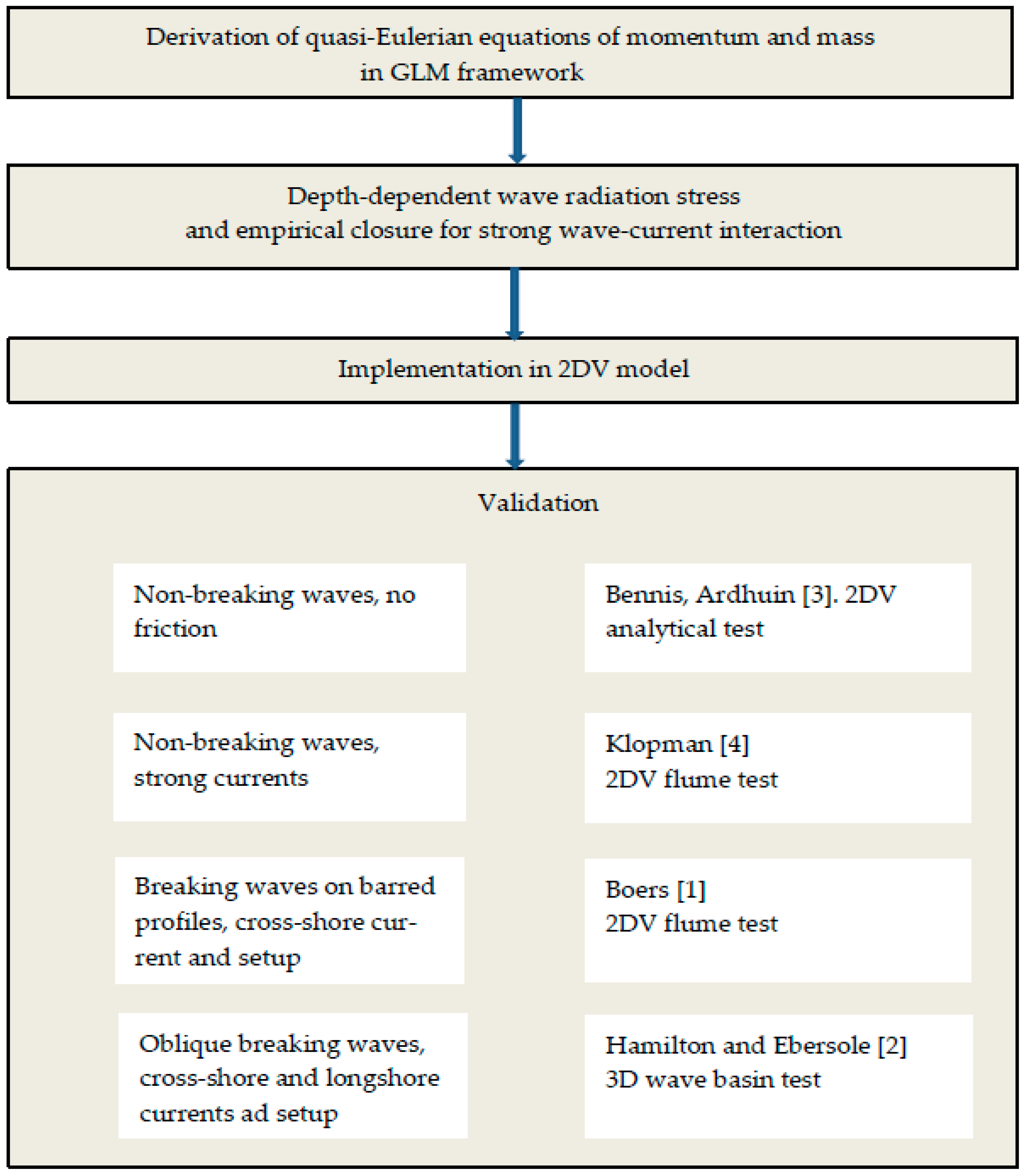
3. Validation of Quasi-Eulerian Mean Equations of Motion

3.1. Model Implementation

In this part, a two-dimensional numerical model is developed based on the quasi-Eulerian mean equations of motion, which were developed in the previous part. The model is written for the variation of hydrodynamic properties in the x- and z-directions (2DV model). All hydrodynamic properties are assumed to be uniform in the y-direction. The accelerations of mean vertical velocity and dissipative forcing are neglected in the vertical momentum equation of mean motion (hydrostatic assumption for the mean flow). The wave properties such as wave amplitude, wave energy, and wave energy dissipation are calculated by wave energy balance equation and roller energy equation given by Roelvink and Reniers [28]. Besides, the horizontal variation of the mean atmospheric pressure at the water surface and Coriolis’ effect are assumed small and neglected.

3.1.1. DV Governing Equations

The quasi-Eulerian mean momentum equations in the 2DV model are given by:

$$\frac{\partial \overline{u}}{\partial t}+\overline{u}\frac{\partial \overline{u}}{\partial x}+\overline{w}\frac{\partial \overline{u}}{\partial z}-{\upsilon }_{mol}\Delta \overline{u}=-g\frac{\partial \overline{\mathsf{\zeta }}}{\partial x}-\frac{\partial \left(\overline{{\tilde{u}}^2}-\overline{{\tilde{w}}^2}\right)}{\partial x}-\frac{\partial \overline{\tilde{u}\tilde{w}}}{\partial z}+\frac{1}{\rho }\left(\frac{\partial {\overline{\tau }}_{11}}{\partial x}+\frac{\partial {\overline{\tau }}_{13}}{\partial z}\right)+O({\epsilon }^3),$$

(25)

$$\frac{\partial \overline{v}}{\partial t}+\overline{u}\frac{\partial \overline{v}}{\partial x}+\overline{w}\frac{\partial \overline{v}}{\partial z}+X_2=-{\upsilon }_{mol}\Delta \overline{v}=-\frac{\partial \overline{\tilde{u}\tilde{v}}}{\partial x}-\frac{\partial \overline{\tilde{v}\tilde{w}}}{\partial z}+\frac{1}{\rho }\left(\frac{\partial {\overline{\tau }}_{21}}{\partial x}+\frac{\partial {\overline{\tau }}_{23}}{\partial z}\right)+O({\epsilon }^3),$$

(26)

where, only molecular viscosity is considered as non-wave dissipative forcing and ${\upsilon }_{mol}$ is molecular viscosity.

The components of turbulence stress tensor are parameterized by:

$${\overline{\tau }}_{11}=\mathsf{\rho }{\upsilon }_h^T\frac{\partial \overline{u}}{\partial x},\begin{array}{cc}& {\overline{\tau }}_{13}=\mathsf{\rho }{\upsilon }_v^T\frac{\partial \overline{u}}{\partial z}\end{array},$$

(27)

$${\overline{\tau }}_{21}=\mathsf{\rho }{\upsilon }_h^T\frac{\partial \overline{v}}{\partial x},\begin{array}{cc}& {\overline{\tau }}_{23}=\mathsf{\rho }{\upsilon }_v^T\frac{\partial \overline{v}}{\partial z}\end{array},$$

(28)

where, ${\upsilon }_h^T$ and ${\upsilon }_v^T$ are horizontal and vertical turbulent viscosities, respectively. In this study, horizontal turbulent viscosity is assumed a constant ${\upsilon }_h^T=1.0\times {10}^{-3}$ m²/s, and vertical turbulent viscosity is assumed a constant-parabolic distribution, i.e.,

$${\upsilon }_v^T(z)=\{\begin{array}{l}\kappa \delta \left(1-\frac{\delta }{h}\right)\begin{array}{cc}{\overline{u}}_{*,c}& if\left(z+h\right)\le \delta \end{array}\\ -\kappa z\left(1+\frac{z}{h}\right){\overline{u}}_{*,c}\begin{array}{cc}& otherwise\end{array}\end{array},$$

(29)

where, $\kappa =0.041$ is the Von Karman constant, ${\overline{u}}_{*,c}=\sqrt{\left|{\overline{\tau }}_c\right|/\mathsf{\rho }}$ is friction velocity, and ${\overline{\tau }}_c$ is the bed shear stress caused by the mean current.

In the condition of stationary waves, the quasi-Eulerian mean continuity equation in the 2DV model is:

$$\frac{\partial \overline{u}}{\partial x}+\frac{\partial \overline{w}}{\partial z}=\frac{\partial {\overline{Z}}^S}{\partial t}-\frac{\partial {\overline{u}}^S}{\partial x}-\frac{\partial {\overline{w}}^S}{\partial z},$$

(30)

If the bed level is fixed then the depth-integrated continuity equation is simplified as:

$$\frac{\partial \overline{\mathsf{\zeta }}}{\partial t}+\frac{\partial }{\partial x}{\displaystyle {\int }_{-h}^{{\overline{\mathsf{\zeta }}}^L}\overline{u}dz}=-\frac{\partial }{\partial x}\left({\displaystyle {\int }_{-h}^{{\overline{\mathsf{\zeta }}}^L}{\overline{u}}^{S}dx}\right),$$

(31)

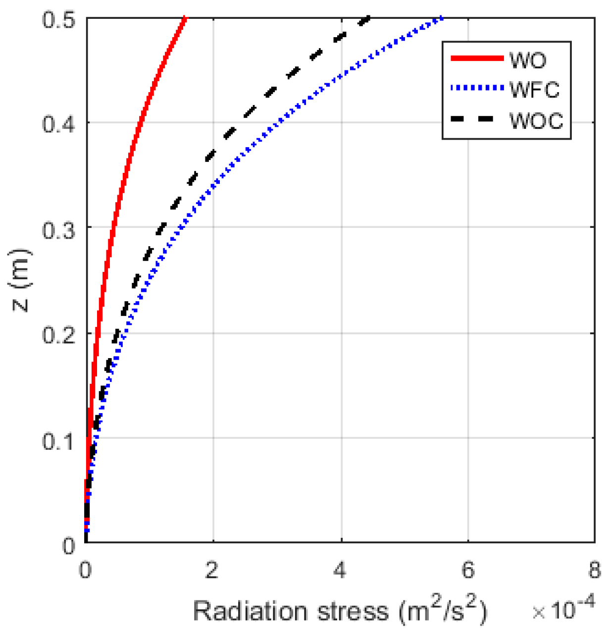
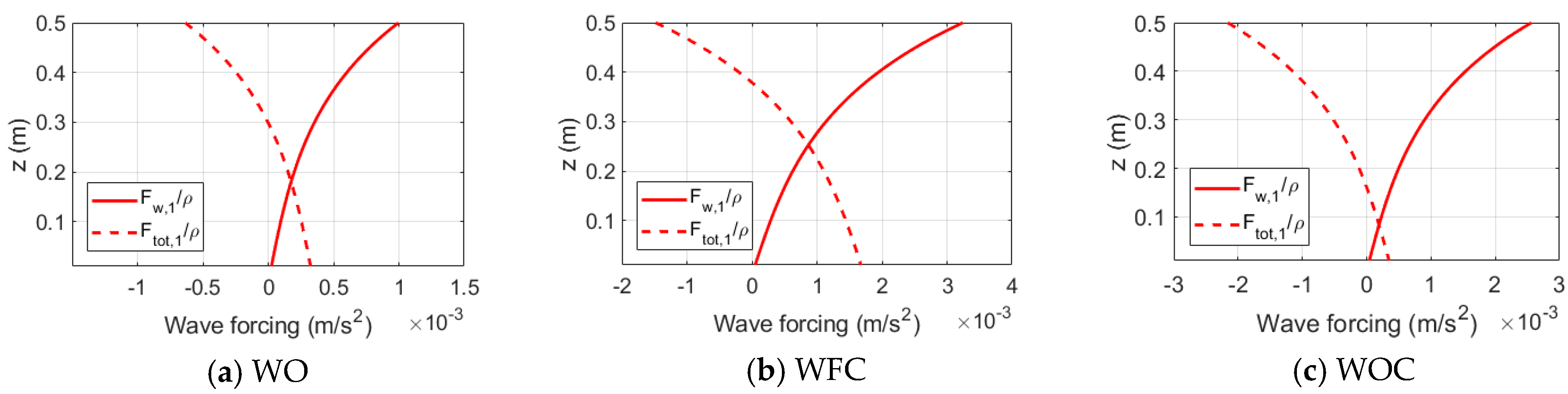
3.1.2. Depth-Dependent Wave Radiation Stress in the 2DV Model

The following formulas are derived with the assumption that all the surface waves are uniform in the y-direction. Components of wave radiation stress tensor in horizontal momentum equations are defined as:

$$S_{xx}=\mathsf{\rho }\left(\overline{{\tilde{u}}^2}-\overline{{\tilde{w}}^2}\right)\begin{array}{ccc}& & \end{array}{S}_{xz}=\mathsf{\rho }\overline{\tilde{u}\tilde{w}},$$

(32)

$$S_{yx}=\mathsf{\rho }\overline{\tilde{v}\tilde{u}}\begin{array}{ccccc}& & & & \end{array}{S}_{yz}=\mathsf{\rho }\overline{\tilde{v}\tilde{w}},$$

(33)

With the assumption of slow modulation of the waves, the shear components of radiation stress tensor can be estimated by a local linear wave theory. The horizontal components of the wave velocity are given by:

$$\tilde{u}=\frac{k_1\sigma a}{k}\frac{\cosh k\left(z+h\right)}{\sinh kh}\cos \left(k_{1}x+k_{2}y-\sigma t\right),$$

(34)

$$\tilde{v}=\frac{k_2\sigma a}{k}\frac{\cosh k\left(z+h\right)}{\sinh kh}\cos \left(k_{1}x+k_{2}y-\sigma t\right),$$

(35)

The vertical component of wave velocity is calculated from the continuity equation for the wave motion:

$$\tilde{w}=\sigma a\frac{\sinh k(z+h)}{\sinh kh}\sin (k_{1}x+k_{2}y-\sigma t)-\frac{k_1}{k^2}\sigma \frac{\partial a}{\partial x}\frac{\sinh k(z+h)}{\sinh kh}\cos (k_{1}x+k_{2}y-\sigma t),$$

(36)

Then, shear components of the wave radiation stress tensor are:

$$S_{xx}=\mathsf{\rho }gk{a}^2\left(\frac{k_1^2}{k^2}\frac{{\cosh }^{2}k(z+h)}{\sinh 2kh}-\frac{{\sinh }^{2}k(z+h)}{\sinh 2kh}\right),$$

(37)

$$S_{yx}=\mathsf{\rho }g{a}^2\frac{k_1{k}_2}{k}\frac{{\cosh }^{2}k(z+h)}{\sinh 2kh},$$

(38)

The vertical distribution of normal components of wave radiation stress in dissipative waves was analyzed by Deigaard and Fredsøe [29]. Their study is restricted to shallow water waves, where the horizontal wave velocity is assumed to be depth-independent. This results in the linear variation of $S_{xz}$ and $S_{yz}$ with depth. Usually, the horizontal wave velocity is a depth-dependent quantity (e.g., wind waves in deep water), in which case more general formulation for $S_{xz}$ and $S_{yz}$ are required. In general, the normal components of wave radiation stress can be decomposed into conservative and decay parts, such as:

$$\overline{\tilde{u}\tilde{w}}={\overline{\tilde{u}\tilde{w}}}_{CS}+{\overline{\tilde{u}\tilde{w}}}_{DC},$$

(39)

$$\overline{\tilde{v}\tilde{w}}={\overline{\tilde{v}\tilde{w}}}_{CS}+{\overline{\tilde{v}\tilde{w}}}_{DC},$$

(40)

where, the subscripts CS and DC represent the conservative and decay parts of the normal components of wave radiation stress, respectively.

(a) Conservative part of the normal component of the wave radiation stress in weak ambient current.

When the ambient current is small in comparison with the near-bed orbital velocity, the conservative part of the normal component of the wave radiation stress can be calculated from Equations (34)–(36) to obtain:

$${\overline{\tilde{u}\tilde{w}}}_{CS}=-\frac{g{k}_1^{2}a\sinh \left(2k(z+h)\right)}{2k^2\sinh 2kh}\frac{\partial a}{\partial x},$$

(41)

$${\overline{\tilde{v}\tilde{w}}}_{CS}=-\frac{g{k}_1{k}_{2}a\sinh \left(2k(z+h)\right)}{2k^2\sinh 2kh}\frac{\partial a}{\partial x},$$

(42)

The above formulas agree with the results obtained by You [30] and Groeneweg [26] when the incident angle of the wave is zero ($\theta =0^0$).

(b) Conservative part of the normal component of the wave radiation stress in a strong ambient current.

As pointed out by Supharatid, Tanaka [31], and Nielsen and You [32], the ambient current has a significant impact on the vertical distribution of wave radiation stress. Therefore, Equations (41) and (42) are no longer suitable in the presence of a strong ambient current. The normal component of the wave radiation stress is enhanced by a factor $C_{WR}=\left(C_{WR,1},C_{WR,2}\right)$ representing the effect of the ambient current. Equations (41) and (42) become:

$${\overline{\tilde{u}\tilde{w}}}_{CS}=-\frac{C_{WR,1}g{k}_1^{2}a\sinh \left(2k(z+h)\right)}{2k^2\sinh 2kh}\frac{\partial a}{\partial x},$$

(43)

$${\overline{\tilde{v}\tilde{w}}}_{CS}=-\frac{C_{WR,2}g{k}_1{k}_{2}a\sinh \left(2k(z+h)\right)}{2k^2\sinh 2kh}\frac{\partial a}{\partial x},$$

(44)

For regular waves, the empirical factors $C_{WR,1}$ and $C_{WR,2}$ are calculated based on the formula, which was proposed by Nielsen and You [32], i.e.,

$$C_{WR,1}=1+100\frac{\overline{u_{*}}}{\sigma a}\frac{\left(z+h\right)}{D},$$

(45)

$$C_{WR,2}=1+100\frac{\overline{v_{*}}}{\sigma a}\frac{\left(z+h\right)}{D},$$

(46)

where, $\left(\overline{u_{*}},\overline{v_{*}}\right)$ is the friction velocity caused by waves and currents, a is the wave amplitude, and $D=h+\overline{\mathsf{\zeta }}$ the mean of total water depth.

As indicated by Ockenden and Soulsby [33], for a substantial part of the time, the bottom shear stresses caused by random waves exceed those of the corresponding regular waves. In this study, Formulas (43) and (44) are modified to apply for random waves as follows:

$$C_{WR,1}=1+100\sqrt{2}\frac{\overline{u_{*}}}{\sigma a}\frac{\left(z+h\right)}{D},$$

(47)

$$C_{WR,2}=1+100\sqrt{2}\frac{\overline{v_{*}}}{\sigma a}\frac{\left(z+h\right)}{D},$$

(48)

where, $a=0.5H_{rms}$ with $H_{rms}$ is the root mean square wave height. The empirical coefficient approximates unity when the ambient current is small in comparison with the near-bed orbital velocity. The friction velocity components caused by waves and currents are calculated by:

$$\overline{u_{*}}=\sqrt{{\overline{\tau }}_{b,1}/\mathsf{\rho }}\begin{array}{ccc}& & \end{array}\overline{v_{*}}=\sqrt{{\overline{\tau }}_{b,2}/\mathsf{\rho }},$$

(49)

where, ${\overline{\tau }}_b=\left({\overline{\tau }}_{b,1},{\overline{\tau }}_{b,2}\right)$ is the total bed-shear stress caused by waves and currents. Simply, the instantaneous total bed shear stress can be decomposed as:

$${\tau }_b={\tau }_w+\left|{\overline{\tau }}_{cw}\right|,$$

(50)

where, ${\tau }_w$ is the wave-induced bed shear stress and ${\overline{\tau }}_{cw}$ is the bed-shear stress caused by the mean current in the presence of waves. In this work, ${\tau }_w$ is calculated based on the formula introduced by Soulsby [34].

For monochromatic waves, shear stress ${\overline{\tau }}_{cw}$ is calculated by:

$${\overline{\tau }}_{cw}=-\frac{1}{2}\mathsf{\rho }{f}_{cw}{\overline{u}}_b\sqrt{{\overline{u}}_b^2+\frac{1}{2}{\left|u_{orb}\right|}^2},$$

(51)

where, $f_{cw}$ is the friction factor of the mean current in the presence of waves [35], $u_b=\left(u_b,v_b\right)$ is the near-bed horizontal velocity, and $\left|u_{orb}\right|$ is the near-bed orbital velocity amplitude.

For random waves, the Formula (51) is modified based on the approximate practical formula of Feddersen, Guza [36], i.e.,

$${\overline{\tau }}_{cw}=-\frac{1}{2}\mathsf{\rho }{f}_{cw}{\overline{u}}_b\sqrt{{(1.16s)}^2+{\overline{u}}_b{}^2},$$

(52)

(c) Decay-related parts of the normal component of the wave radiation stress.

Outside the bottom boundary layer, the decay-related part of wave radiation stress gradient is caused by the dissipative forcing, i.e.,

$$\frac{\partial {\overline{\tilde{u}\tilde{w}}}_{DC}}{\partial z}=-\frac{F_{br,1}(z)}{\mathsf{\rho }}-\frac{F_{mx,1}(z)}{\mathsf{\rho }},$$

(53)

$$\frac{\partial {\overline{\tilde{v}\tilde{w}}}_{DC}}{\partial z}=-\frac{F_{br,2}(z)}{\mathsf{\rho }}-\frac{F_{mx,2}(z)}{\mathsf{\rho }},$$

(54)

where, $F_{br}=\left(F_{br,1},F_{br,2}\right)$ represents the effect of breaking wave and roller wave, and $F_{mx}=\left(F_{mx,1},F_{mx,2}\right)$ represents the wave-induced mixing. In this work, the vertical distribution of the wave-induced forcing terms $F_{br}$ and $F_{mx}$ is estimated by empirical formulas proposed by Uchiyama, McWilliams [14].

At the bottom, the wave energy is dissipated due to bottom friction. According to Longuet-Higgins [37]:

$${\overline{\tilde{u}\tilde{w}}}_{DC}(-h)=-\frac{k_1{D}_f}{\mathsf{\rho }\sigma },$$

(55)

$${\overline{\tilde{v}\tilde{w}}}_{DC}(-h)=-\frac{k_2{D}_f}{\mathsf{\rho }\sigma },$$

(56)

Defining $F_{tot}$ as the total of wave-induced mixing and current-induced turbulent forcing, i.e.,

$$\frac{F_{tot,1}}{\mathsf{\rho }}=\frac{1}{\mathsf{\rho }}\left(F_{mx,1}+\frac{\partial {\overline{\tau }}_{11}}{\partial x}+\frac{\partial {\overline{\tau }}_{13}}{\partial z}\right),$$

(57)

$$\frac{F_{tot,2}}{\mathsf{\rho }}=\frac{1}{\mathsf{\rho }}\left(F_{mx,2}+\frac{\partial {\overline{\tau }}_{21}}{\partial x}+\frac{\partial {\overline{\tau }}_{23}}{\partial z}\right),$$

(58)

The total of wave-induced forcing caused by the conservative part of the wave radiation stress and breaking wave and roller wave-induced forcing $F_w$ is:

$$\frac{F_{w,1}}{\mathsf{\rho }}=-\left[\frac{\partial \left(\overline{{\tilde{u}}^2}-\overline{{\tilde{w}}^2}\right)}{\partial x}+\frac{\partial {\overline{\tilde{u}\tilde{w}}}_{CS}}{\partial z}\right]+\frac{F_{br,1}}{\mathsf{\rho }},$$

(59)

$$\frac{F_{w,2}}{\mathsf{\rho }}=-\left[\frac{\partial \overline{\tilde{u}\tilde{v}}}{\partial x}+\frac{\partial {\overline{\tilde{v}\tilde{w}}}_{CS}}{\partial z}\right]+\frac{F_{br,2}}{\mathsf{\rho }},$$

(60)

Then, the sum $\left(F_w+F_{tot}\right)$ represents the total effects of wave and turbulence on the mean current.

3.1.3. Bottom Boundary Layer Thickness in the Wave–Current Interaction Condition

In the condition of waves combined with current, Van Rijn [35] proposed the following formula:

$$\mathsf{\delta }=0.2A_{orb}{\left(A_{orb}/k_n\right)}^{-0.25},$$

(61)

where, $k_n=30z_0$ is the Nikuradse roughness.

However, Equation (61) does not account for the effect of near-bed mean current on the bottom boundary layer thickness. Therefore, it is only suitable if the near-bed mean current is small in comparison with the near-bed orbital velocity. When the near-bed current is significant and is comparable to the orbital velocity the following formula is proposed:

$$\mathsf{\delta }=0.2A_{orb}{\left(A_{orb}/k_n\right)}^{-0.25}\left(1+\left|{\overline{u}}_b\right|/\left|u_{orb}\right|\right),$$

(62)

It is clear that when $\left|{\overline{u}}_b\right|\ll \left|u_{orb}\right|$ the Formula (62) reduces to Formula (61).

3.2. Numerical Approximation

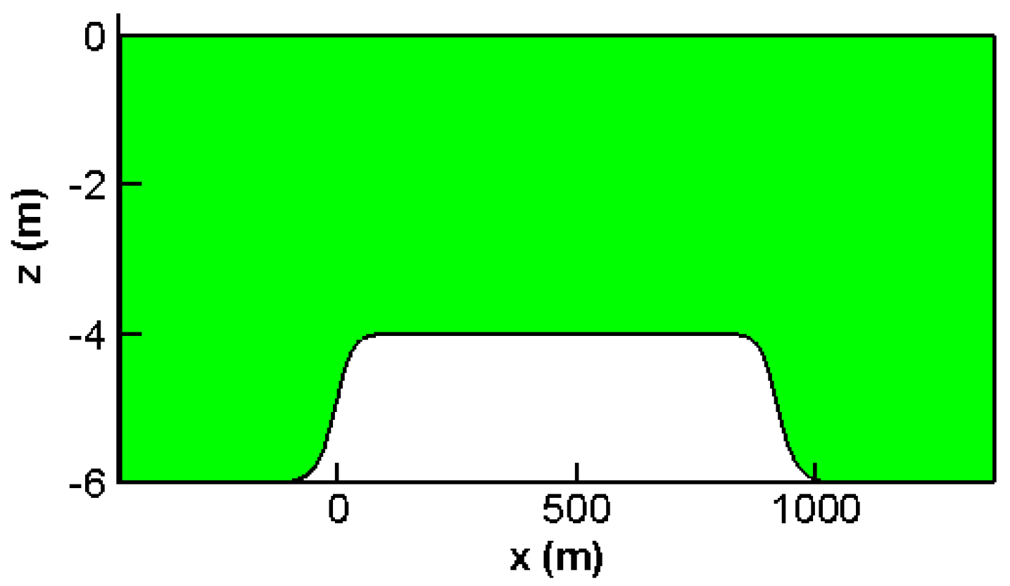
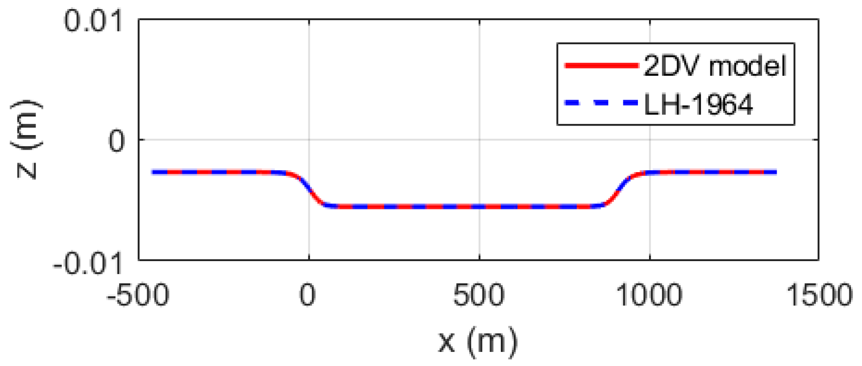
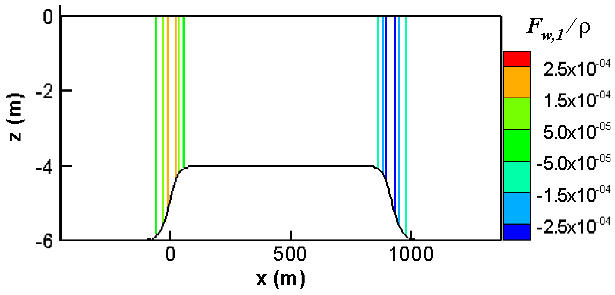
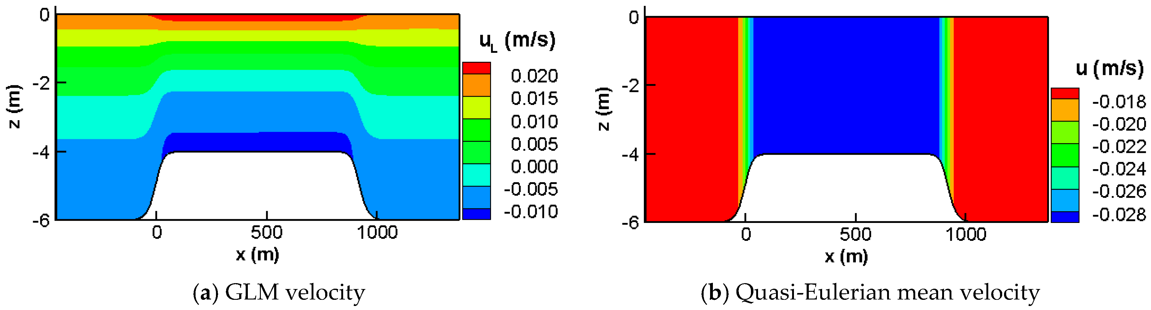
The 2DV equations of mean motion are discretized based on the finite difference method on a fully staggered grid (C-grid). An implicit numerical scheme has been used to discretize the equations. Finally, the tridiagonal matrix algorithm (Thomas algorithm) has been used to solve these equations. In the model, the water level is approximated at the grid point $\left(i,k\right)$, the horizontal component of velocity at $\left(i+1/2,k\right)$, and the vertical component of velocity at $\left(i,k+1/2\right)$. The advection terms are approximated following the principles described in Stelling and Busnelli [38]. This method ensures the conservation of properties near large local gradient areas. The 2DV model developed in this study is a time-domain model starting from rest and simulating to equilibrium in all cases.

3.3. Adiabatic Test

The adiabatic test, described in Bennis, Ardhuin [39], is a seemingly simple but challenging test of the derived equations since any imbalance leads to strong spurious circulations. This test was applied firstly by Ardhuin, Rascle [19]. In this, a steady monochromatic small-amplitude wave propagates over a slope without dissipation. This test has an exact solution by solving Laplace’s equation for the instantaneous velocity potential with given bottom, surface, and lateral boundary conditions [19]. In the work of Ardhuin, Rascle [19], the adiabatic test was solved by using the NTUA-nl2 model (National Technical University of Athens numerical model) developed by Belibassakis and Athanassoulis [40]. The quasi-Eulerian mean current is depth-uniform.

3.3.1. Bathymetry

The bathymetry was symmetrical and varied slowly from 4 to 6 m in the x-direction, and was uniform in the y-direction (Figure 2). The maximum bottom slope was 2.6 × 10⁻², and the reflection coefficient was $R=1.4\times {10}^{-9}$, so the reflected wave in the momentum balance could be neglected [19].

3.3.2. Boundary Conditions

At the boundary, a regular wave with a height of 1.02 m and a period of 5.26 s was imposed. This is also the wave that was used by Ardhuin, Rascle [19], and Bennis, Ardhuin [39] to test their models in the adiabatic condition. The mean water level at the outflow boundary is given by:

$$\overline{\mathsf{\zeta }}=-\frac{k{a}^2}{2\sinh 2kD},$$

(63)

At the inflow boundary, the quasi-Eulerian mean velocity is vertical uniform and given by:

$$\overline{u}(z)=-\frac{1}{h+{\overline{\mathsf{\zeta }}}^L}{\displaystyle {\int }_{-h}^{{\overline{\mathsf{\zeta }}}^L}{\overline{u}}^S(z)dz},$$

(64)

At the outflow boundary, the Neumann boundary condition is applied, i.e.,

$$\frac{\partial \overline{u}}{\partial x}=-\frac{\partial {\overline{u}}^S}{\partial x},$$

(65)

3.3.3. Numerical Results

Figure 3 shows the spatial distribution of Stokes drift in the x-direction. It shows that the Stokes drift was constant over the horizontal bed and the magnitude of the Stokes drift increased with a decrease in water depth and vice versa.

The comparison of the mean water level calculated by the numerical model and calculated by the formula of Longuet-Higgins and Stewart [3] is given in Figure 4. It shows a perfect agreement between the two calculation methods.

In the adiabatic condition, the total forcing $F_{tot,1}$ was zero. The vertical distribution of wave forcing term $F_{w,1}/\mathsf{\rho }$ is presented in Figure 5. It shows that wave-induced forcing $F_{w,1}/\mathsf{\rho }$ was zero when the waves propagated over a flat bed. On a sloping bed, this forcing was not nil and was distributed uniformly over depth. Then, the total forcing $\left(F_{w,1}+F_{tot,1}\right)$ was depth-uniform in the adiabatic condition.

When the wave propagated over a slope, the change of the wave height led to the change of Stokes drift. Due to the conservation of mass and momentum, the quasi-Eulerian mean velocity also changed. However, the vertical integration of total flow was still unchanged, and in this case, it equaled zero:

$${\displaystyle {\int }_{-h}^{{\overline{\mathsf{\zeta }}}^L}{\overline{u}}^{L}dz}=0,$$

(66)

Since all dissipative forcing was absent, the quasi-Eulerian mean horizontal velocity was uniformly distributed over the vertical. However, the GLM velocity inherited the non-uniformity from the Stokes drift (Figure 6a). Figure 6b presents the quasi-Eulerian mean velocity calculated with the 2DV model. It proves that quasi-Eulerian mean equations of motion passed the adiabatic test.

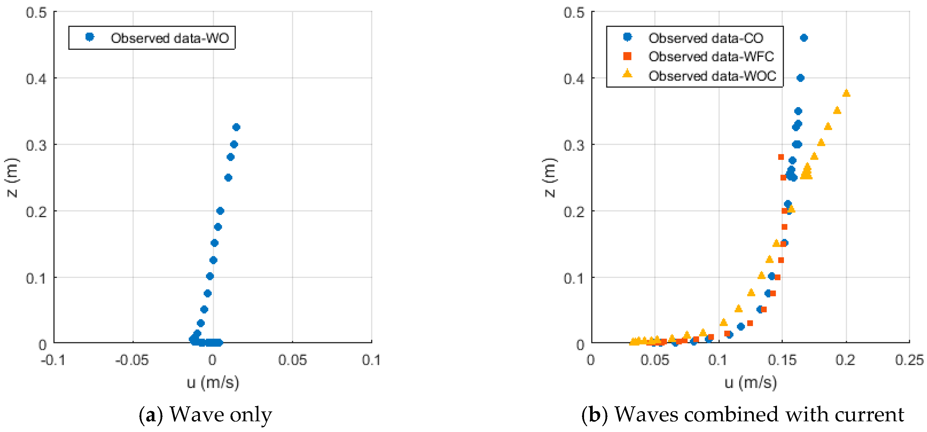
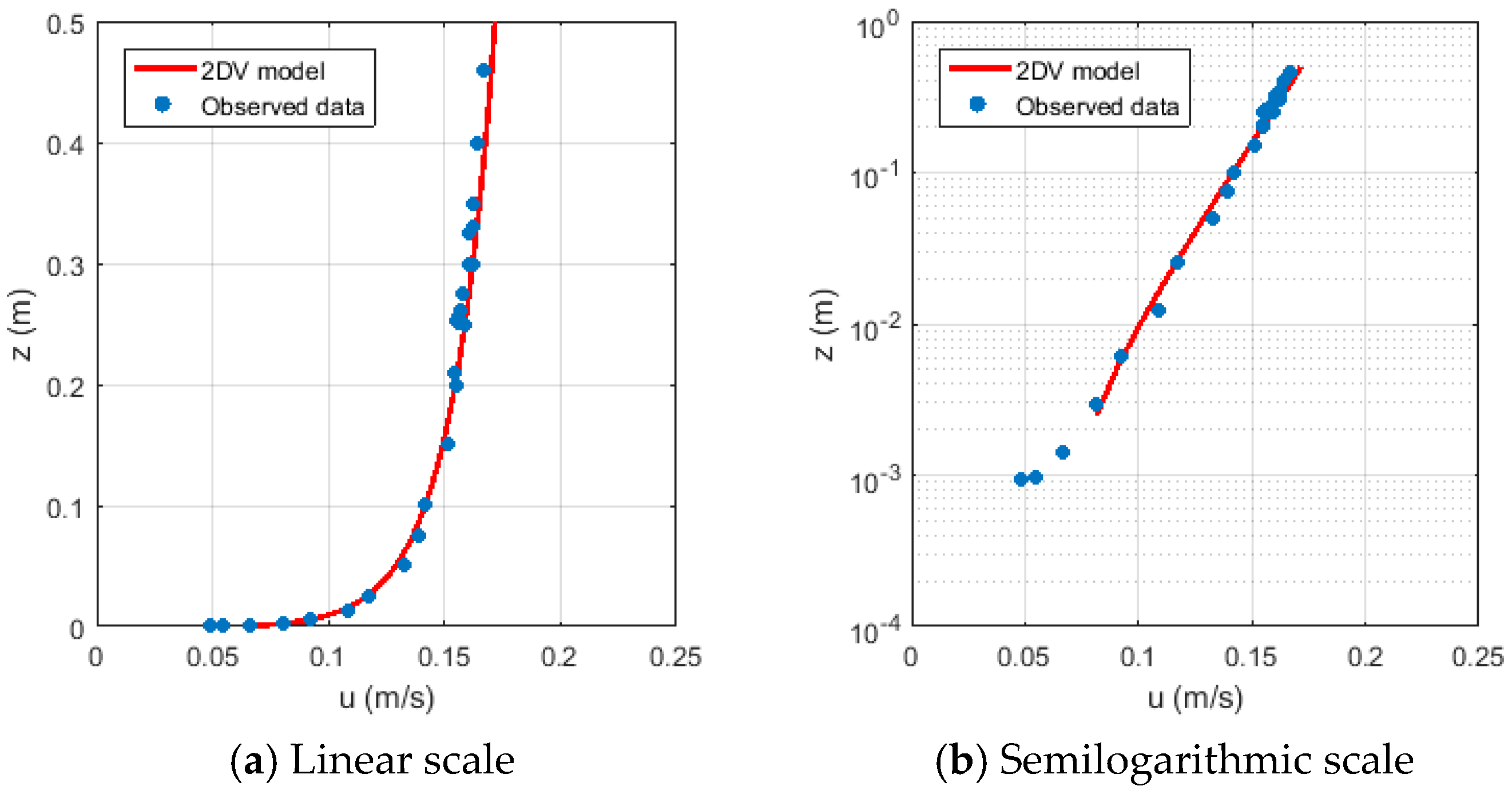
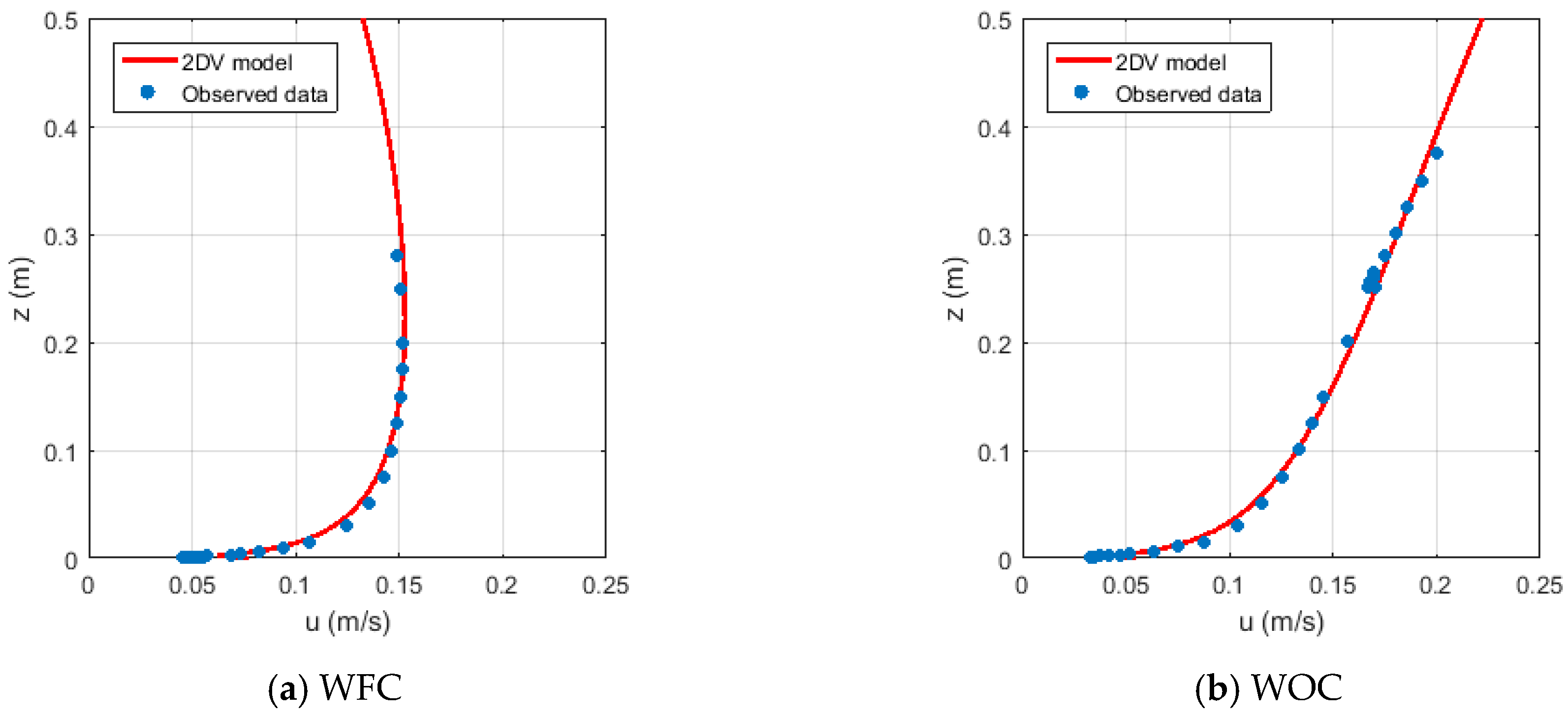
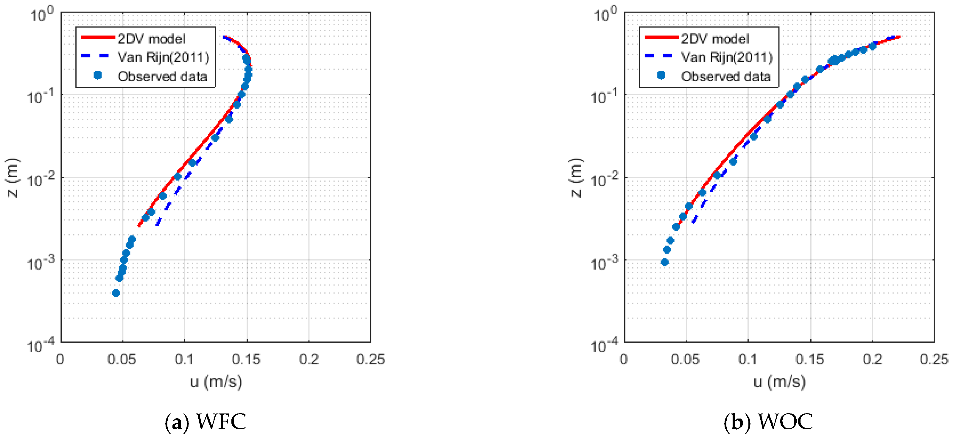
3.4. Mean Current in the Presence of Non-Breaking Waves

In the experiment of Klopman [41], the vertical distribution of the mean current was measured in three different types of waves: monochromatic waves, bichromatic waves, and random waves. The experiments were performed for four conditions of ambient currents: currents only (CO), waves only (WO), waves following currents (WFC), and waves opposing currents (WOC). The wave height was chosen so that no wave breaking took place. Therefore, the bottom friction plays an important role in the vertical distribution of the mean current. In the following, the experimental data for random waves were employed to validate the 2DV numerical model.

3.4.1. Input Parameters

The experiment was performed in a wave flume that has a horizontal flat bottom. The flume was 45 m long, 1 m wide, and 0.5 m deep. The total discharge was kept constant: $Q=0$ m³/s for the case of wave-only, and $Q=0.08$ m³/s for the remaining cases. The properties of the random waves at the wave paddle are given in

Table 1. Wave properties at the paddle.

Wave Type	Tp (s)	Hrms (m)	h (m)
Random	1.7	0.1	0.5

.

The flow velocities were measured at the center of the channel, i.e., 22.5 m from the wave paddle. Two laser-Doppler velocimetry flow meters (LDVs) were used to measure flow velocity components. The vertical distributions of Eulerian-mean velocities measured at the center of the flume are presented in Figure 6.

In the WO condition (Figure 7a), the wave propagated from the right-hand side to the left-hand side. It shows that the wave-induced streaming near the bed was in the same direction as the propagation of the surface waves. The horizontal mean velocity changes sign at a height of approximately 0.13 m from the bed [41]. Outside the bottom streaming layer, the mean velocity varied almost linearly. In Figure 7b, the vertical distribution of horizontal mean velocity is presented in three conditions: CO, WFC, and WOC. It shows that vertical profiles of the mean current changed significantly in the presence of surface waves. In the WFC condition, the velocity shear $\partial \overline{u}/\partial z$ was negative in the upper part of the water column (z/h > 0.4). In the WOC condition, the mean velocity decreased near the bed (z/h < 0.4), and increased near the surface (z/h > 0.4) in comparison with the current-only condition.

By linear extrapolation of the velocities in a semilogarithmic scale, Klopman [41] obtained the friction velocity $u_{*}\approx 7.3\times {10}^{-3}$ m/s. The vertical distribution of the Reynolds shear stress $\overline{-u^t{w}^t}$ is present in Figure 8. The bottom shear stress was estimated by Klopman [41] about ${\overline{\tau }}_b/\mathsf{\rho }=4.6\times 10^{-5}$ m²/s², corresponding to the friction velocity of $u_{*}=\sqrt{{\overline{\tau }}_b/\mathsf{\rho }}\approx 6.7\times {10}^{-3}$ m/s. Then, the friction velocity calculated from the bed shear stress was slightly smaller than obtained from the velocity profile.

3.4.2. Boundary Conditions

In the model, the shear stress is assumed to vanish at the mean water surface, since non-breaking waves are considered, i.e.,

$${\left[\left({\upsilon }_v+K_{fr}\right)\frac{\partial \overline{u}}{\partial z}\right]}_{z=\overline{\mathsf{\zeta }}}=0,$$

(67)

where, ${\upsilon }_v={\upsilon }_v^T+{\upsilon }_{mol}$. At the bottom, the bottom boundary condition is given by:

$${\left[\left({\upsilon }_v+K_{fr}\right)\frac{\partial \overline{u}}{\partial z}\right]}_{z=-h+\mathsf{\delta }}=-\frac{k{D}_f}{\mathsf{\rho }\sigma }-\frac{{\overline{\tau }}_{cw}}{\mathsf{\rho }},$$

(68)

At the outflow boundary, the boundary condition for the mean water level and the mean current is given by:

$$\overline{\mathsf{\zeta }}=-\frac{k{a}^2}{2\sinh 2kh},$$

(69)

$$\frac{\partial \overline{u}}{\partial x}=-\frac{\partial {\overline{u}}^S}{\partial x},$$

(70)

At the inflow boundary, the quasi-Eulerian mean velocity is given by:

$$\overline{u}(z)=\frac{1}{h+{\overline{\mathsf{\zeta }}}^L}{\overline{Q}}^L-{\overline{u}}^S(z),$$

(71)

where, ${\overline{Q}}^L$ is the mean of total discharge through the pipe.

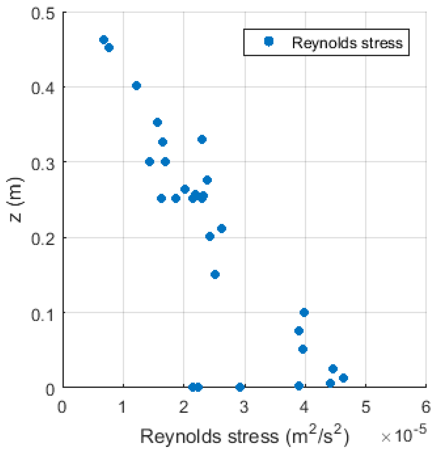
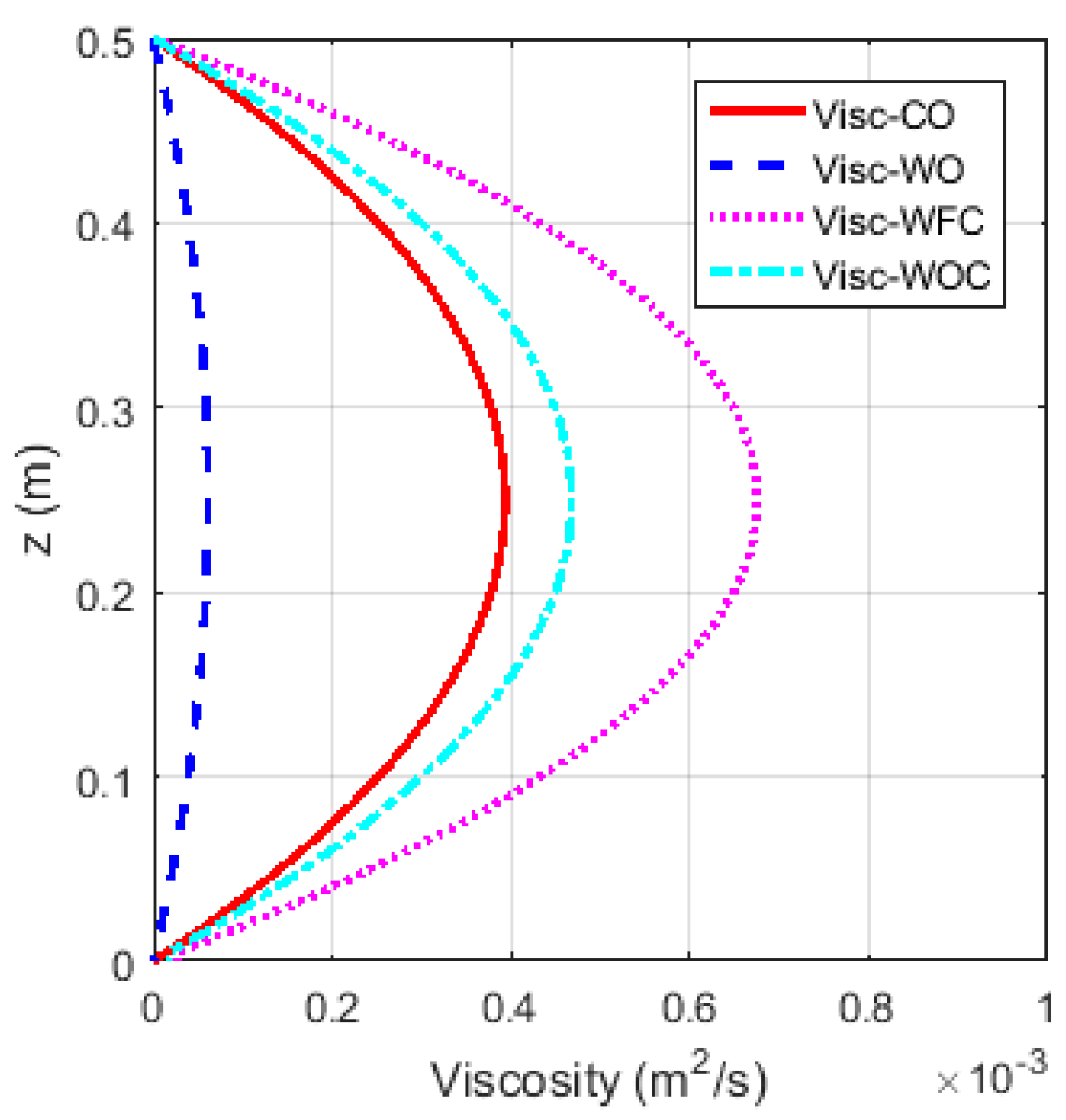
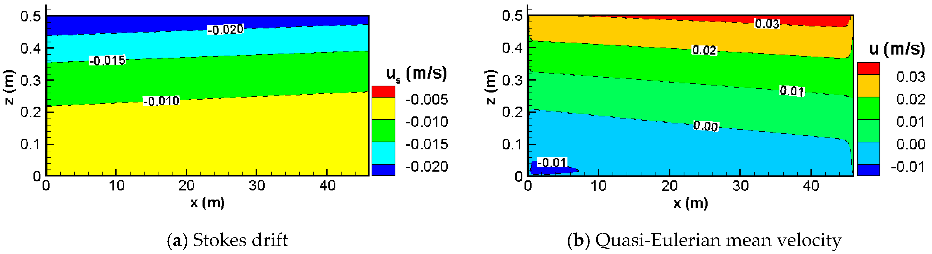
3.4.3. The Numerical Results

The experiment of Klopman [41] is simulated by the 2DV model with spatial steps of $\Delta x=0.15 \mathrm{m}$, $\Delta z=0.0025 \mathrm{m}$, and a time step of $\Delta t=0.5 \mathrm{s}$. In the experiment, due to small technical issues, there was uncertainty in the measured discharge (see Klopman [41] for more detail). However, these errors were not corrected in his document. Generally, the measured discharge is expressed as a total of the real discharge and error discharge, i.e.,

$$Q_{measured}=Q_{real}+Q_{err},$$

(72)

where, $Q_{real}$ is the real discharge through the wave flume, $Q_{measured}$ is the measured discharge, and $Q_{err}$ is the error of flow discharge. In CO condition, it found that when $Q_{err}$ approximates to 0.003 m³s⁻¹ (3.75% of the real discharge) a good agreement between numerical results and experimental data was obtained. In waves combined with current conditions, the error of flow discharge is assumed similar to the current only condition. In the WO condition, flow discharge $Q_{err}$ is zero by definition. In all tests, the bed roughness is kept constant $z_0=4.0\times {10}^{-5}$ m, corresponding to a Nikuradse roughness of $k_n=1.2\times {10}^{-3}$ m. In

Table 2. Bottom boundary thickness $\delta$ in different waves and current conditions.

Conditions	Formula (62) $(\times {10}^{-3} \mathbf{m})$	Van Rijn [35] $(\times {10}^{-3} \mathbf{m})$
CO	0.1	0.1
WO	1.3	1.3
WFC	5.3	3.6
WOC	4.9	3.6

, the bottom boundary thickness is presented. In the condition of waves combined with current, bottom boundary thickness $\delta$ was calculated by two methods: the formula of Van Rijn [35] and its modified Formula (62). The results are presented in Table 2.

Table 3. Characteristics of the near-bed mean flow.

Conditions	$\left|{\overline{\mathit{u}}}_{\mathit{b}}\right|$ $(\times {10}^{-2} \mathbf{m}/\mathbf{s})$	$\left|{\overline{\mathit{\tau }}}_{\mathit{b}}\right|$ $(\times {10}^{-2} {\mathbf{kgm}}^2/{\mathbf{s}}^2)$	${\mathit{u}}_{\ast }$ $(\times {10}^{-2} \mathbf{m}/\mathbf{s})$
CO	8.16	5.4	0.74
WO	0.9	0.21	0.13
WFC	8.10	37.67	1.94
WOC	5.86	24.6	1.56

presents the characteristics of the mean flow near the bed calculated by the 2DV model. It shows that bottom stress in conditions of waves combined with the current was much higher than that in conditions of WO and CO. This is because momentum mixing under wave-current interaction conditions was much higher than in conditions of both WO and CO (see for instance the discussion in Chapter 3 of [42]).

The vertical distribution of Reynolds turbulent viscosity is presented in Figure 9.

It shows that the viscosity in the WFC condition was bigger than in the WOC condition, and viscosity in waves combined with current conditions was bigger than in the CO condition. Moreover, the viscosity in the WO condition was much smaller than for other conditions.

In Figure 10, the conservative part of $\overline{\tilde{u}\tilde{w}}$ in different conditions of waves combined with the current was plotted. It clearly shows that the ambient current had a significant impact on the normal component of the wave radiation stress. Moreover, the conservative part of the normal component of wave radiation stress $\overline{\tilde{u}\tilde{w}}$ in the condition of the following waves was slightly bigger than that in the condition of the opposing waves.

In non-breaking waves, the wave-induced forcing term $F_{w,1}/\mathsf{\rho }$ only represents the effect of the conservative part of the wave radiation stress. Figure 11a–c show the vertical distributions of forcing term $F_{w,1}/\mathsf{\rho }$ and mixing term $F_{tot,1}/\mathsf{\rho }$ at the center of the wave flume. In all three tests, i.e., WO, WFC, and WOC, the forcing $F_{w,1}$ is completely compensated by total mixing $F_{tot,1}$ at any water depth level. The total of these two forcing terms, i.e., $\left(F_{w,1}+F_{tot,1}\right)$, is depth-uniform in the non-breaking wave condition.

Figure 12 shows the vertical distribution of the Reynolds turbulent stress at the center of the wave flume. Near the bed, the turbulent stress calculated by the 2DV numerical model was about ${\overline{\tau }}_b/\mathsf{\rho }\approx 54.4\times {10}^{-6}$ m²/s², and the corresponding friction velocity was $7.4\times {10}^{-3}$ m/s (

Table 4. Wave properties at the offshore boundary.

Experiment	Hs (m)	Tp (s)
Test 1B	0.206	2.03
Test 1C	0.103	3.3.3

), which was in good agreement with the friction velocity obtained from the mean velocity profile by Klopman [41], i.e., $7.3\times {10}^{-3}$ m/s.

The spatial distribution of the quasi-Eulerian mean velocity calculated with the 2DV model in the condition of CO is given in Figure 13. The (vertically uniform) inflow boundary was specified at position $x=0$ m.

The comparison between numerical results and experimental data in the middle of the flume is given in Figure 14. The comparison is given in both the linear scale and semilogarithmic scale. It shows that the mean current profile calculated with the 2DV model closely followed the experimental data. The agreement was good not only in the upper part of the water column but also close to the bed.

In Figure 15, the spatial distributions of Stokes drift and quasi-Eulerian mean velocity in the WO condition are presented. In this, surface waves are imposed at $x=45$ m and propagated towards the left. The Stokes drift was in the direction of the waves, whereas the quasi-Eulerian mean velocity was in the opposite direction. The magnitude of Stokes drift and quasi-Eulerian mean velocity decreased in the wave propagation direction due to the effect of bottom friction. However, the momentum transport of total flow through any vertical section was zero.

The comparison between the quasi-Eulerian mean velocity calculated with the 2DV model and experimental data in the WO condition is given in Figure 16. It shows a very good agreement between model results and experimental data in the whole vertical section even on both linear scale and semilogarithmic scale. The near-bed wave-induced streaming is in the wave propagation direction. The mean horizontal velocity varied near-linearly from above the bottom streaming layer up to the mean surface level.

The spatial distribution of quasi-Eulerian mean velocity in conditions of WFC and WOC are presented in Figure 17a,b. In the case of WFC, the magnitude of the mean velocity was not the biggest at the water surface but located inside the water column. In the case of WOC, the magnitude of velocity increased from the bottom to the water surface.

Figure 18a,b shows the comparisons between experimental data and numerical model results under the condition of waves combined with the current in a linear scale. It shows that the vertical profile of the mean velocity calculated by the 2DV model fit well with experimental data in the whole water column. The agreement holds for both WFC and WOC conditions.

In Figure 19a,b, the semilogarithmic scale is employed to see the agreement between the 2DV model results and experimental results. It shows that the agreement between the 2DV model results and experimental data was very good even in the area very close to the bed. Besides, the mean current velocity profiles using the boundary layer thickness formulation proposed by Van Rijn [35] (Equation (61)) were also plotted (dashed line). The result calculated by the modified formulation (62) was better than the result calculated by the formulation of Van Rijn [35], especially in the region close to the bed. It is noticed that the formula to calculate boundary layer thickness $\mathsf{\delta }$, i.e., Formula (62), is an extension of the formula proposed by Van Rijn [35] (Formula (61)). In Formula (38), the effect of near-bed current is accounted for when calculating $\mathsf{\delta }$. Table 2 presents boundary layer thickness $\mathsf{\delta }$ in different conditions of waves combined with the current. In the wave-only condition, Formulas (38) and (37) are identical. However, the difference between them is significant in cases of a strong ambient current. Comparison presents in Figure 18 suggest that near-bed current should be accounted for to calculate bottom boundary layer thickness, especially in the case of a strong ambient current.

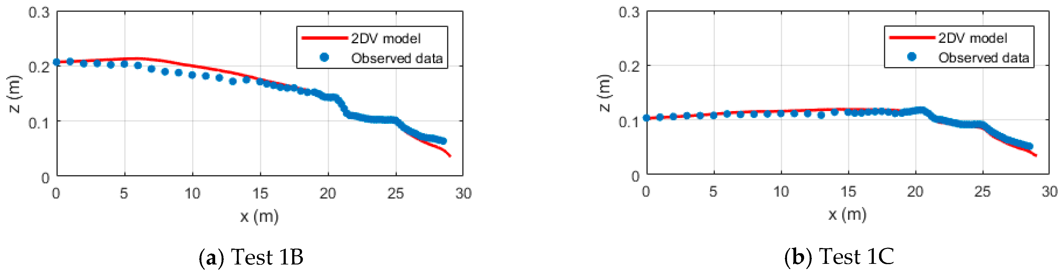
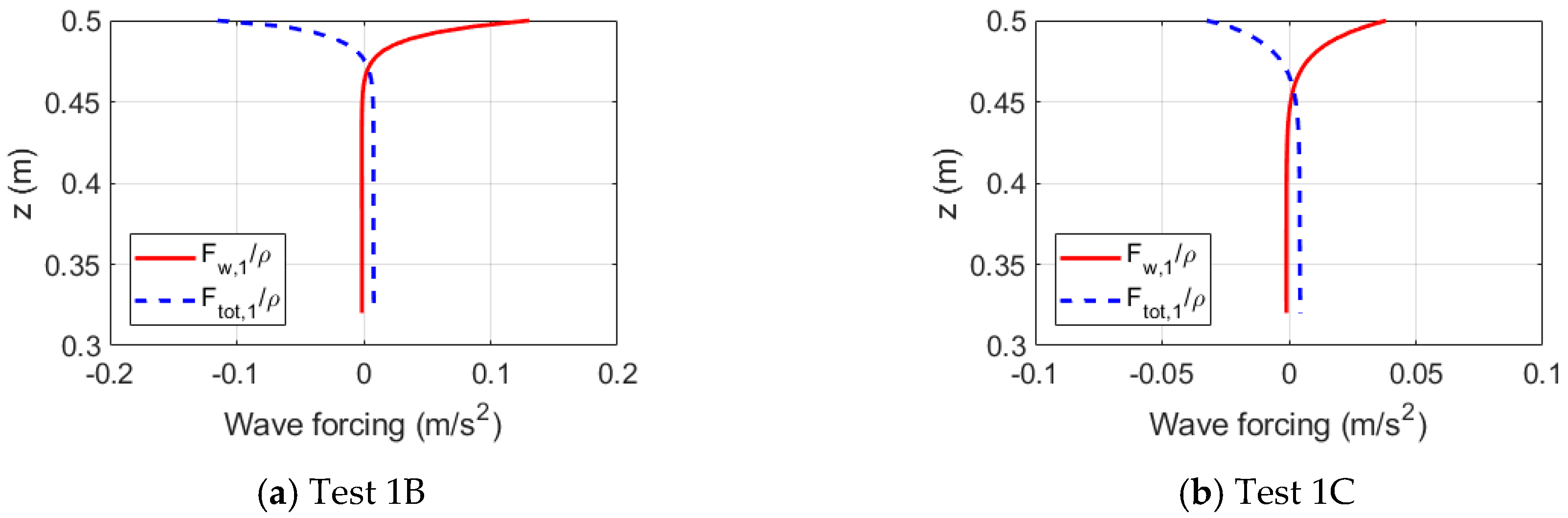
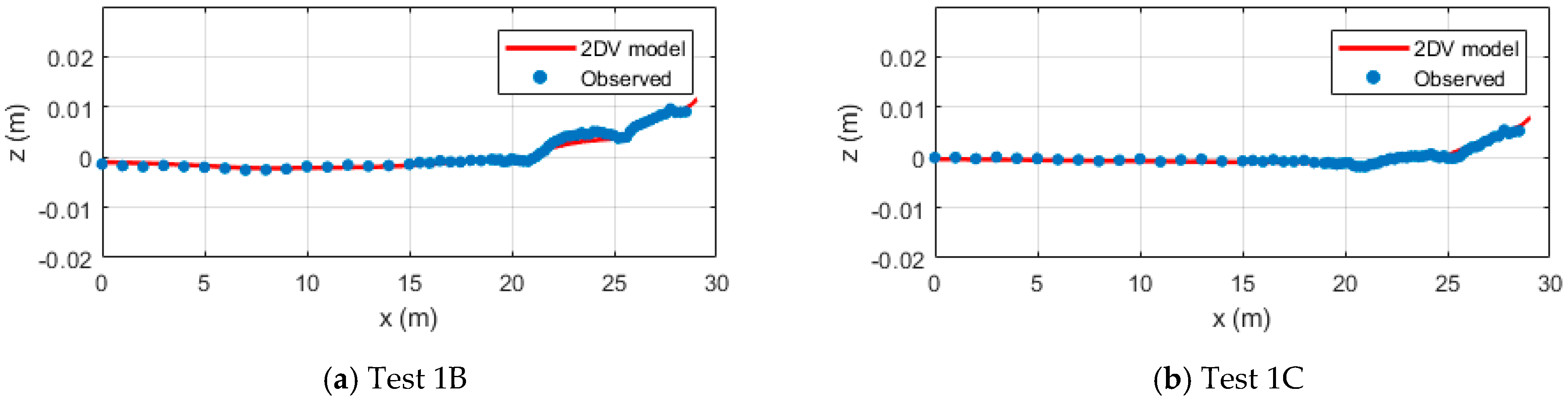
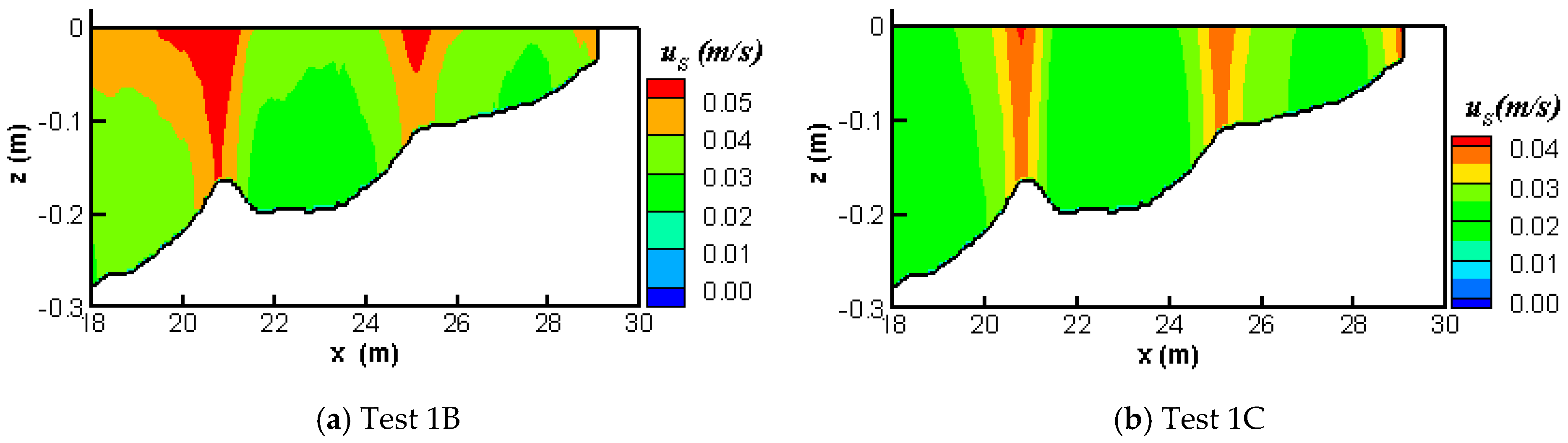
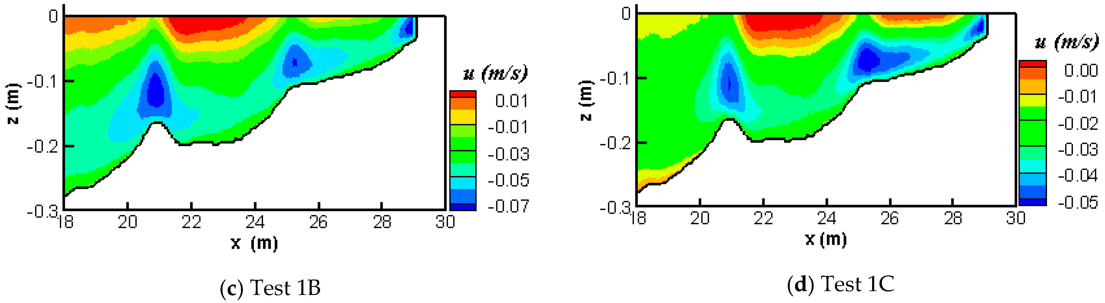
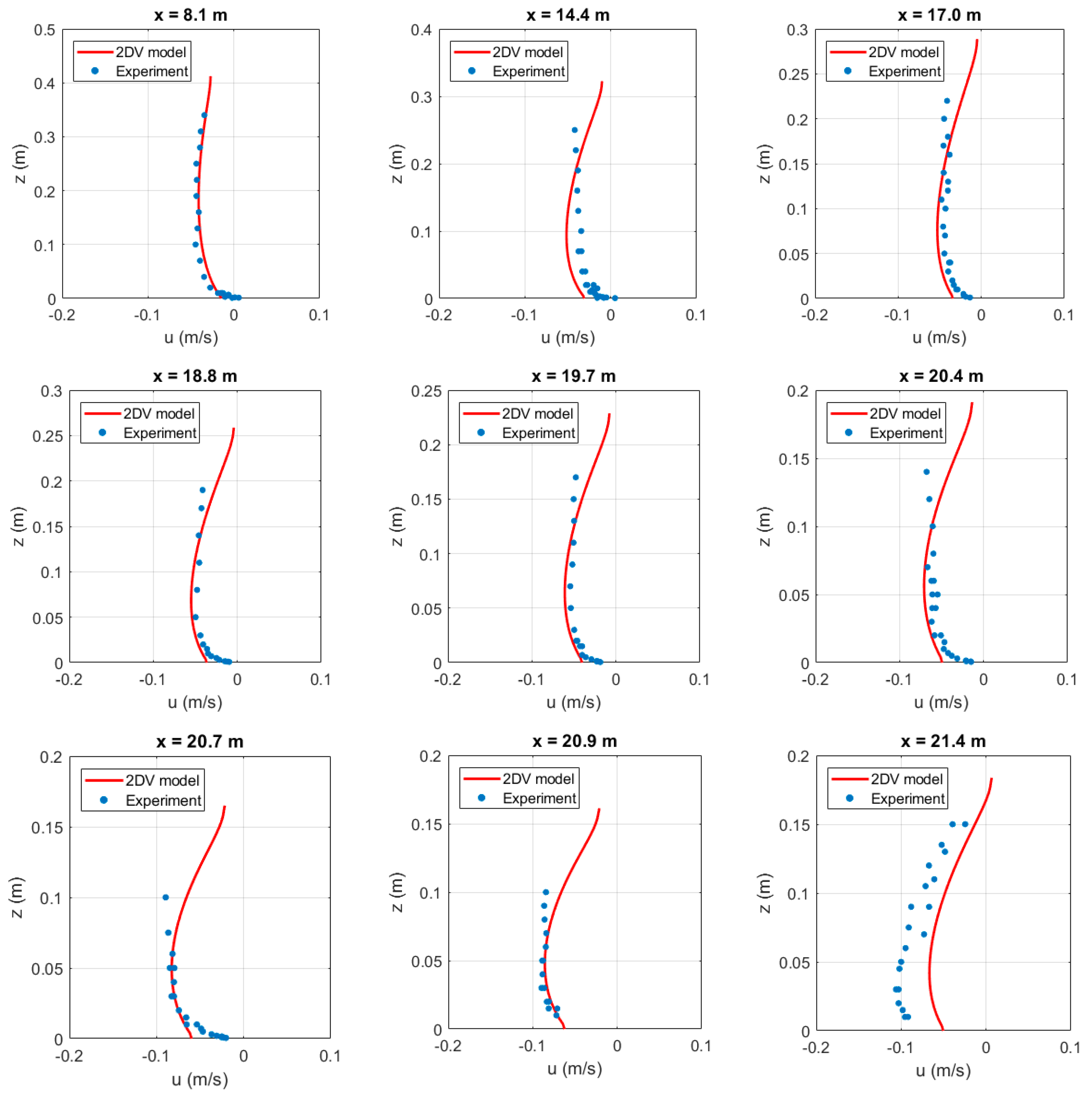
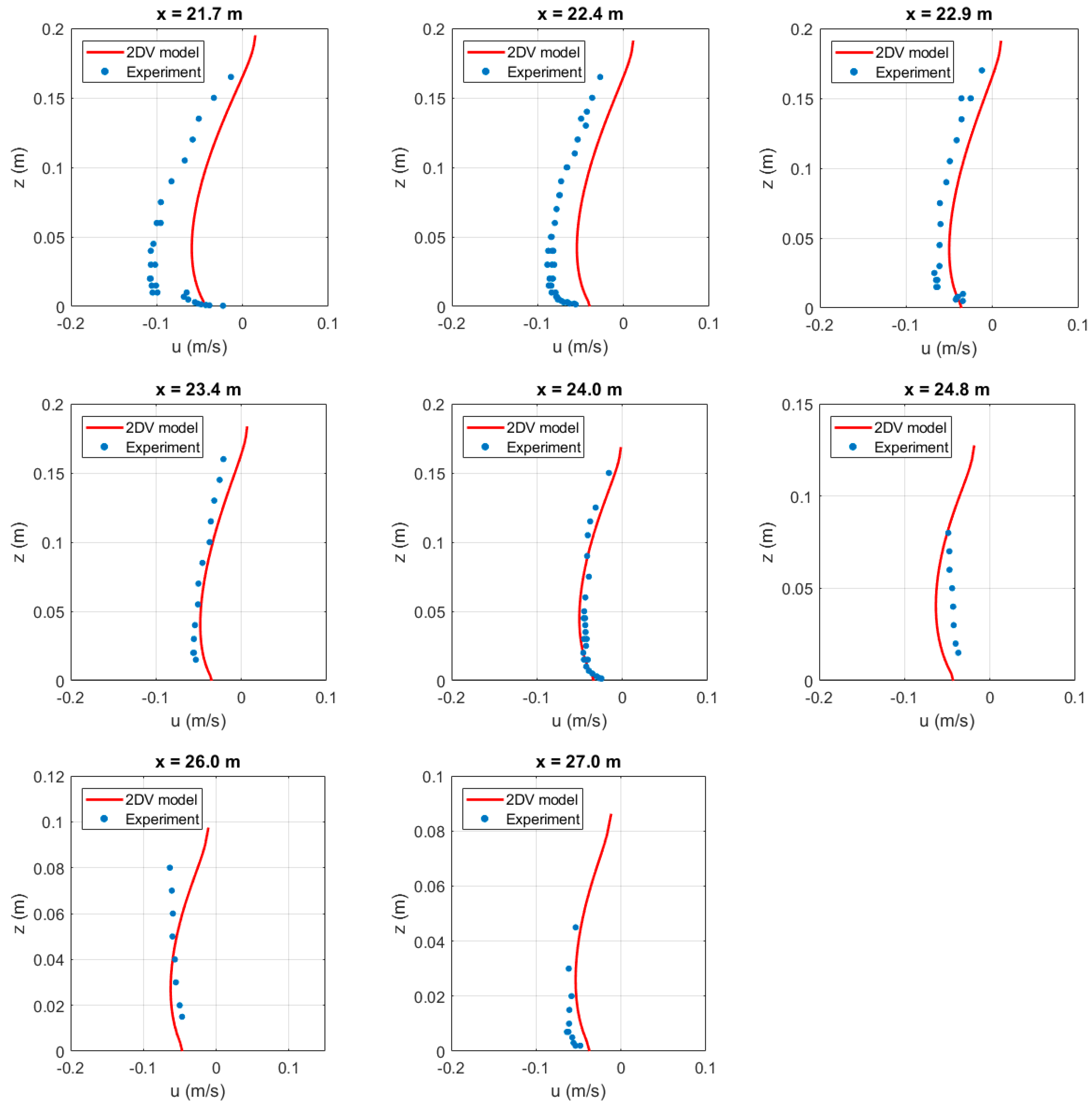
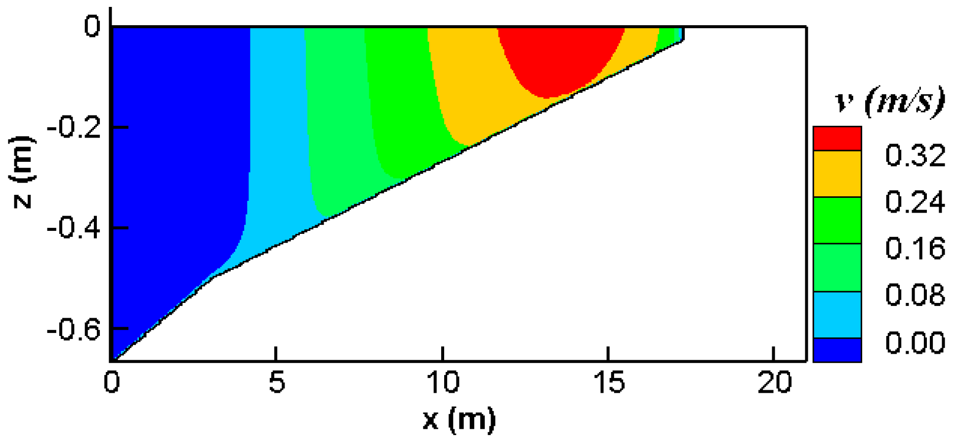
3.5. Breaking Waves Propagating in a Wave Flume

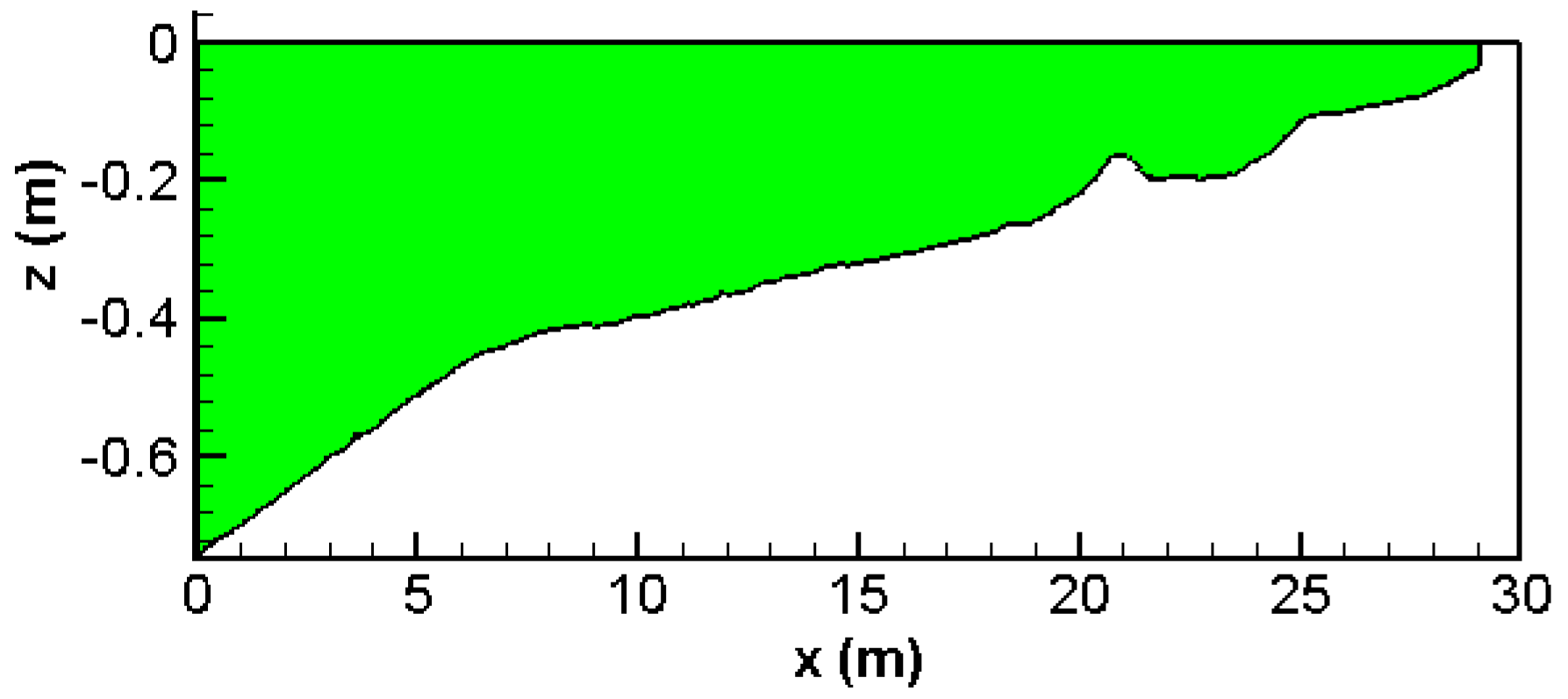
3.5.1. Bathymetry and the Wave Properties at the Boundary

The experiment of Boers [43] was carried out in a wave flume with dimensions of 40 m long, 1.05 m high, and 0.8 m wide. The bottom of the flume is filled with sand and mortar on the top layer. Two breaker bars are designed at the bottom. The still water level was fixed at the level z = 0 m. The bottom profile of the calculation area is depicted in Figure 20.

Two wave conditions with the highest and lowest wave height at the boundary in the experiment of Boers [43] were employed in this work (tests 1B and 1C). The properties of the waves at the offshore boundary are given in Table 4, where $H_s$ was the significant wave height of the waves.

3.5.2. Boundary Conditions

(a) Surface and bottom boundary conditions:

At the GLM water surface, the total shear stress is assumed to vanish, i.e.,

$${\left[\left({\upsilon }_v+K_{fr}+K_b\right)\frac{\partial \overline{u}}{\partial z}\right]}_{z={\overline{\mathsf{\zeta }}}^L}=0,$$

(73)

where, ${\upsilon }_v={\upsilon }_{mol}+{\upsilon }_v^T$

At the bed, the momentum dissipated by bottom friction is assumed to be transferred to the vertical mixing, i.e.,

$${\left[\left({\upsilon }_v+K_{fr}+K_b\right)\frac{\partial \overline{u}}{\partial z}\right]}_{z=-h+\mathsf{\delta }}=-\frac{k_1{D}_f}{\mathsf{\rho }\sigma }-\frac{{\overline{\tau }}_{cw,x}}{\mathsf{\rho }},$$

(74)

(b) Lateral boundary conditions:

The quasi-Eulerian mean water level at the offshore boundary is:

$$\overline{\mathsf{\zeta }}=-\frac{k{a}^2}{2\sinh 2kD},$$

(75)

The quasi-Eulerian mean velocity at the offshore boundary is:

$$\overline{u}(z)=-\frac{1}{h+{\overline{\mathsf{\zeta }}}^L}{\displaystyle {\int }_{-h}^{{\overline{\mathsf{\zeta }}}^L}{\overline{u}}^S(z^{\prime })d{z}^{\prime }},$$

(76)

At the land boundary, the GLM velocity in the cross-shore direction is zero then:

$$\overline{u}(z)=-{\overline{u}}^S(z),$$

(77)

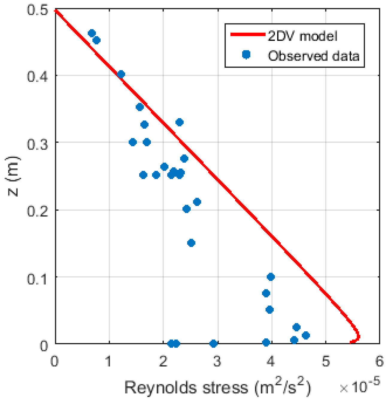
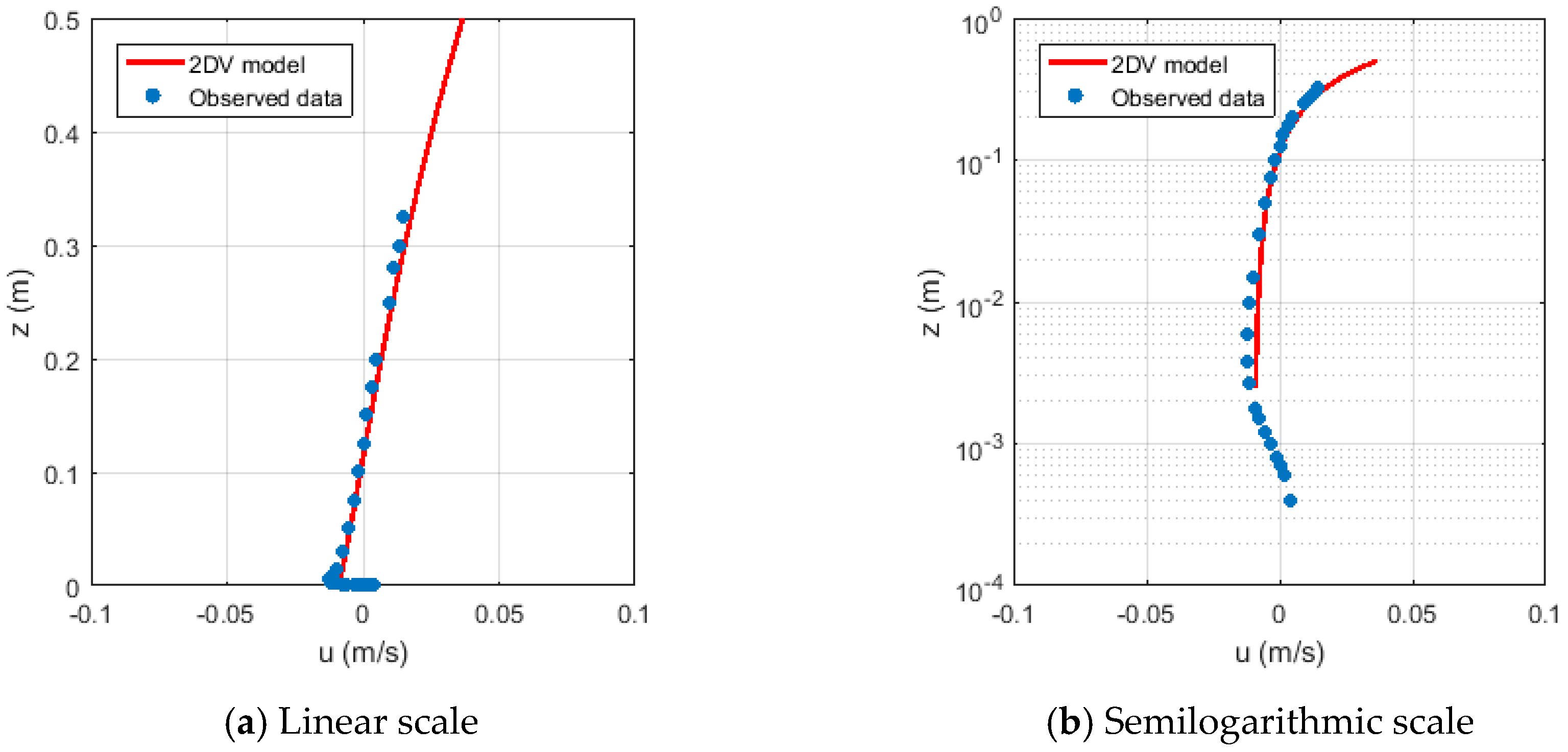
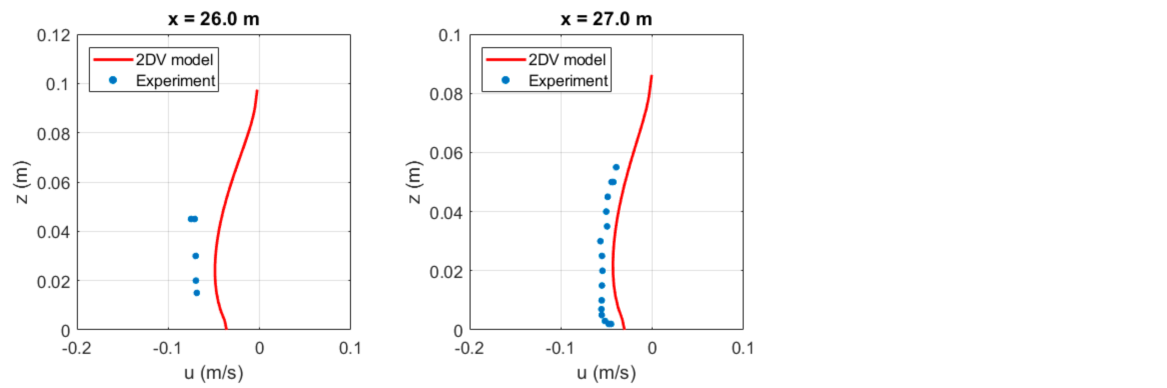
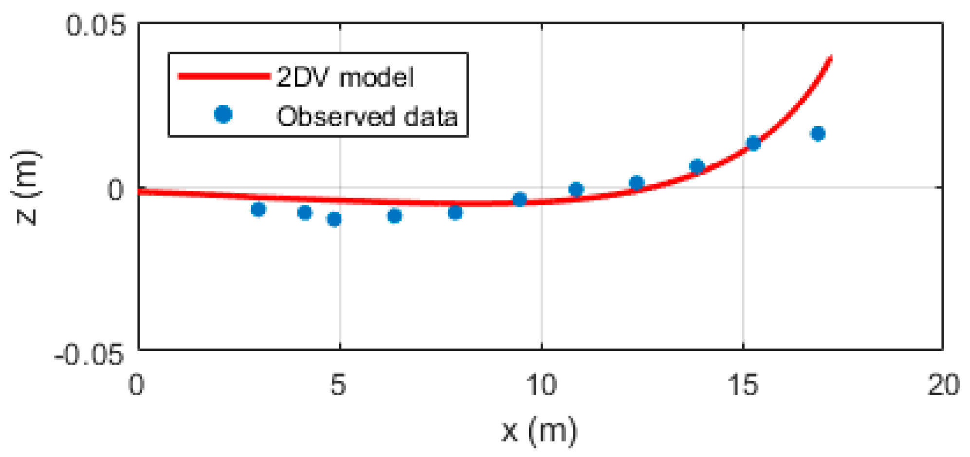
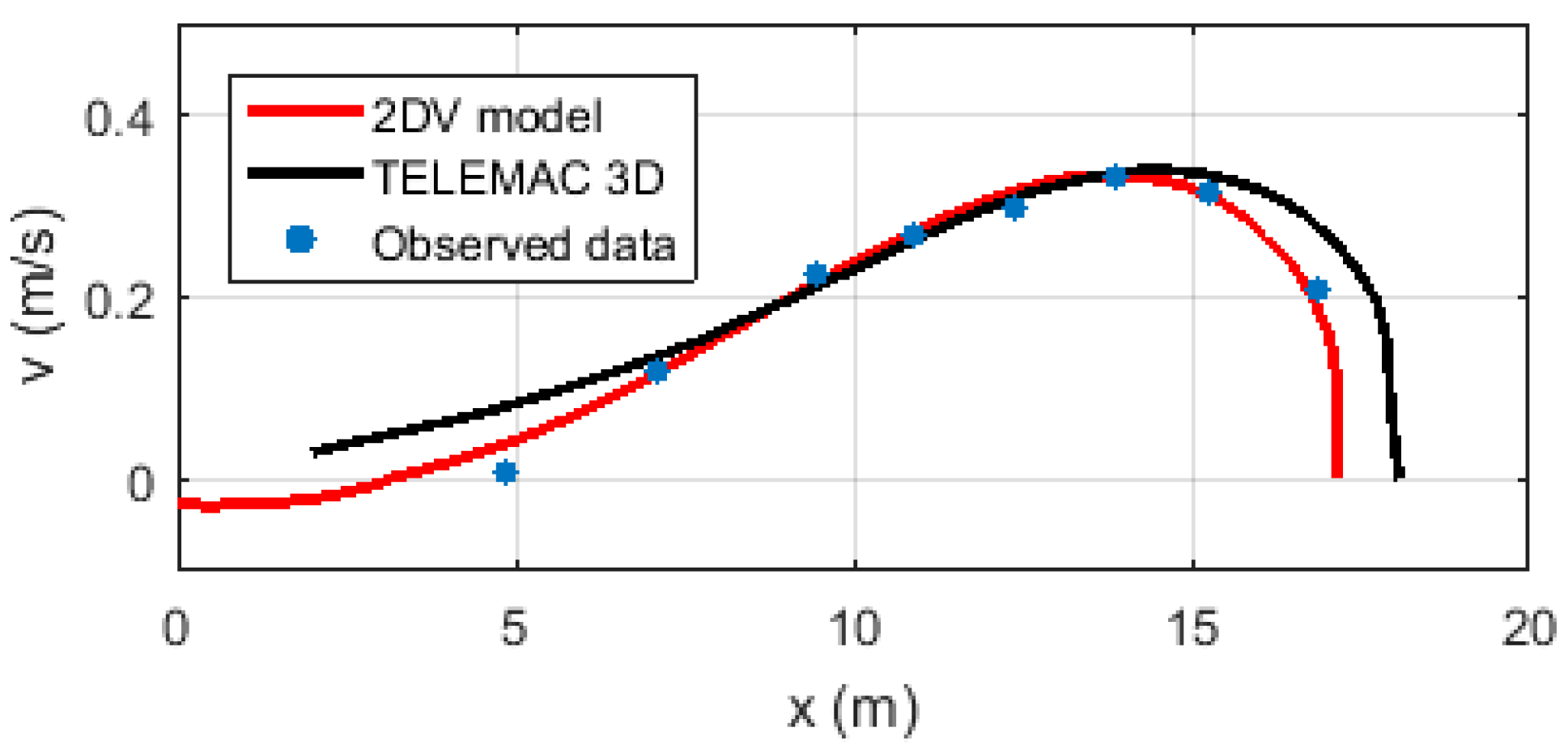
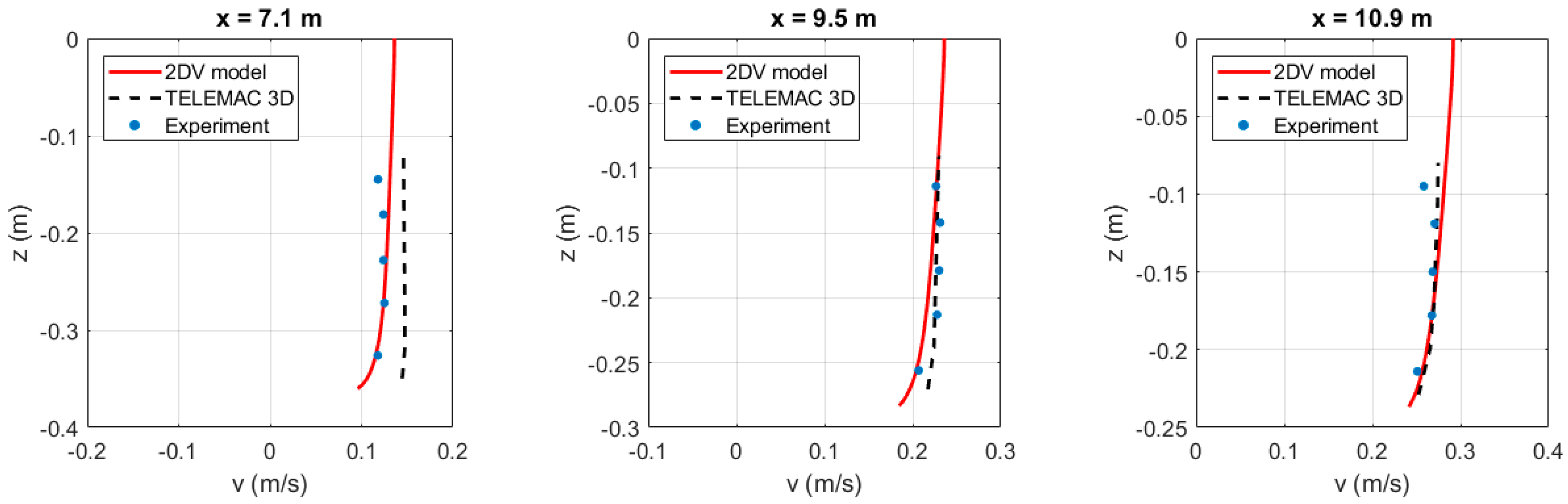
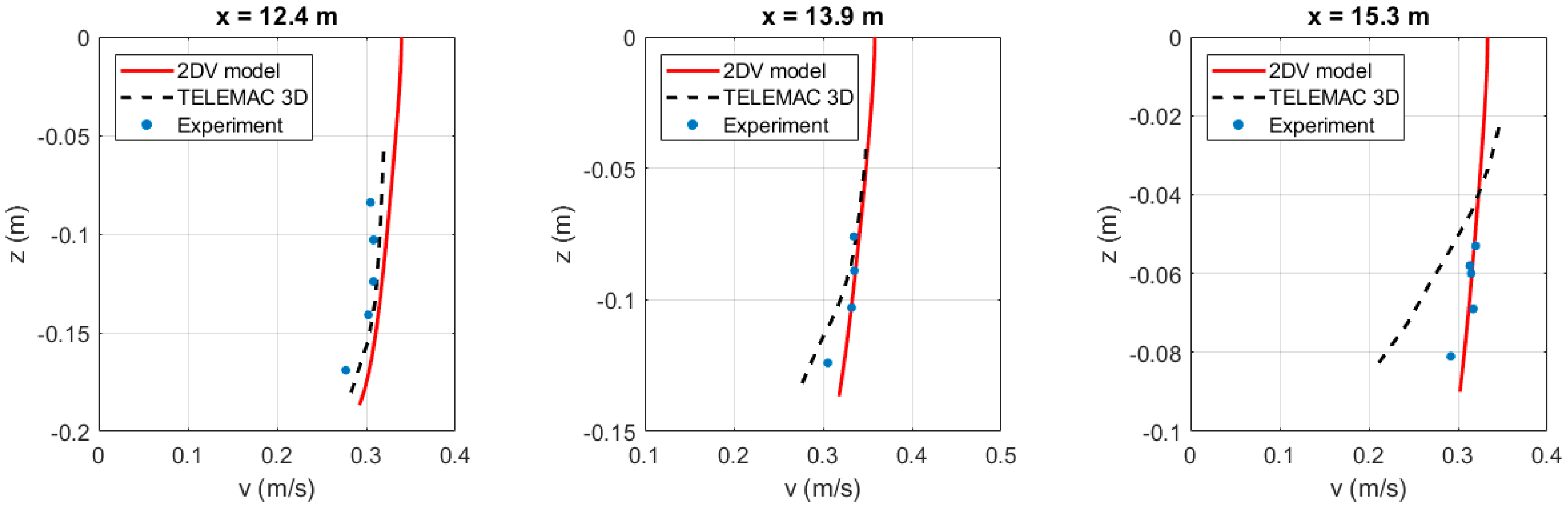
3.5.3. Model Validation

In the experiment, the cross-shore distribution of significant wave height was calculated from the zeroth-order spectral moment of surface elevation [43], that is:

$$H_s=4\sqrt{{\displaystyle {\int }_0^{f_N}S(f)df}},$$

(78)

where, $S(f)$ is the spectral energy density, and $f_N$ is Nyquist frequency of the measurements ($\approx 10 \mathrm{Hz}$).

The significant wave height in the 2DV numerical model is calculated from the wave energy balance equation. In Figure 21, the spatial distributions of significant wave height in tests 1B and 1C are presented. In this, the dots present the experimental data, and the solid line presents the numerical model results. It shows that the numerical model results fit well with measured data. In test 1B, the experimental data was slightly lower than the model results in the region from x = 5 m to x = 14 m. In test 1C, the recirculation was rather small then a better agreement between two kinds of data was obtained.

Figure 22a,b show the vertical distribution of forcing term $F_{w,1}/\mathsf{\rho }$ and total mixing term $F_{tot,1}/\mathsf{\rho }$ at $x=22.9 \mathrm{m}$. It shows that the wave-induced forcing $F_{w,1}/\mathsf{\rho }$ is completely balanced by total mixing $F_{tot,1}/\mathsf{\rho }$. Total forcing $\left(F_{w,1}+F_{tot,1}\right)$ is depth—uniform in breaking wave conditions.

The comparison of the mean water level calculated by the 2DV numerical model with measured data is given in Figure 23. In both tests, the calculated mean water level fits well with measured data even in the breaking wave area.

The horizontal distribution of Stokes drifts and quasi-Eulerian mean velocities calculated by the 2DV model is presented in Figure 24. At the locations near the sandbars, it shows that the quasi-Eulerian mean velocity was increased in the shoreward direction. This is due to the increase of Stokes drift in the onshore direction. In the breaking wave area, it shows a large vertical shear of the quasi-Eulerian mean velocity.

The comparison between quasi-Eulerian mean velocities calculated by the 2DV numerical model and measured data along the wave flume is given in Figure 25 and Figure 26.

Overall, the 2DV model simulated quite well the vertical distribution of the mean velocity. In comparison with test 1B, the model results for the test 1C show a better agreement with experimental data, especially near the sandbars. It suggests that empirical formulas of Uchiyama, McWilliams [14] can be applied well for small-amplitude waves. For the waves of high-amplitude, these empirical formulas just give qualitative results in the breaking zone and further research on the wave forcing in breaking wave areas is needed.

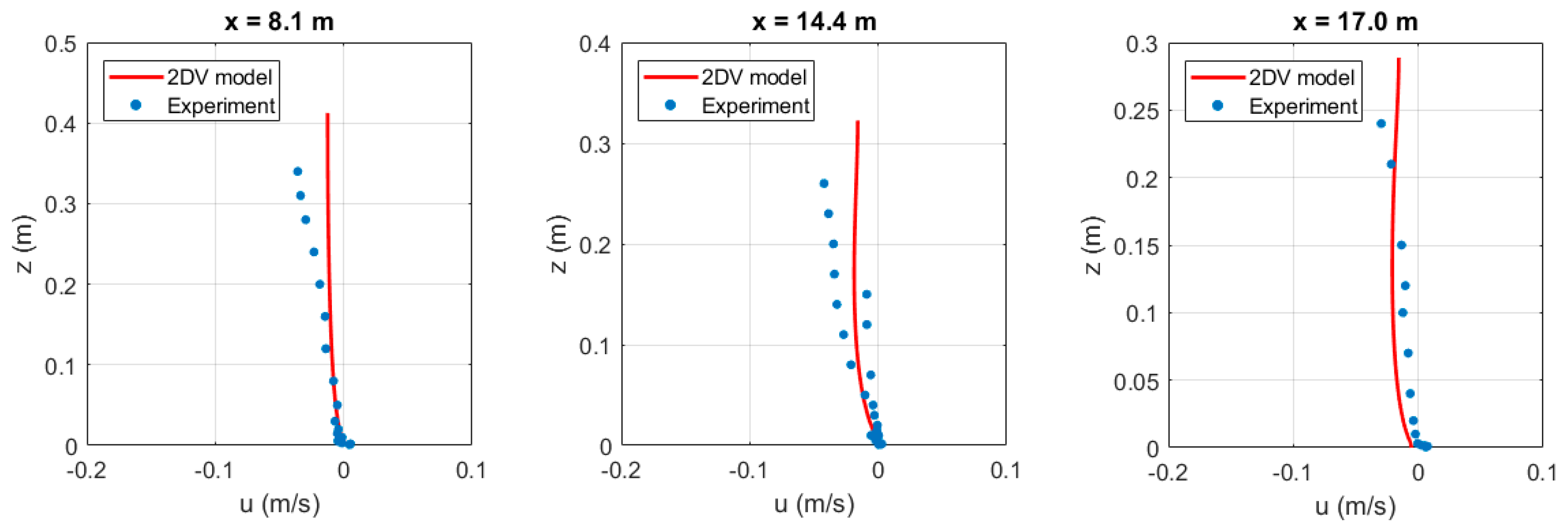
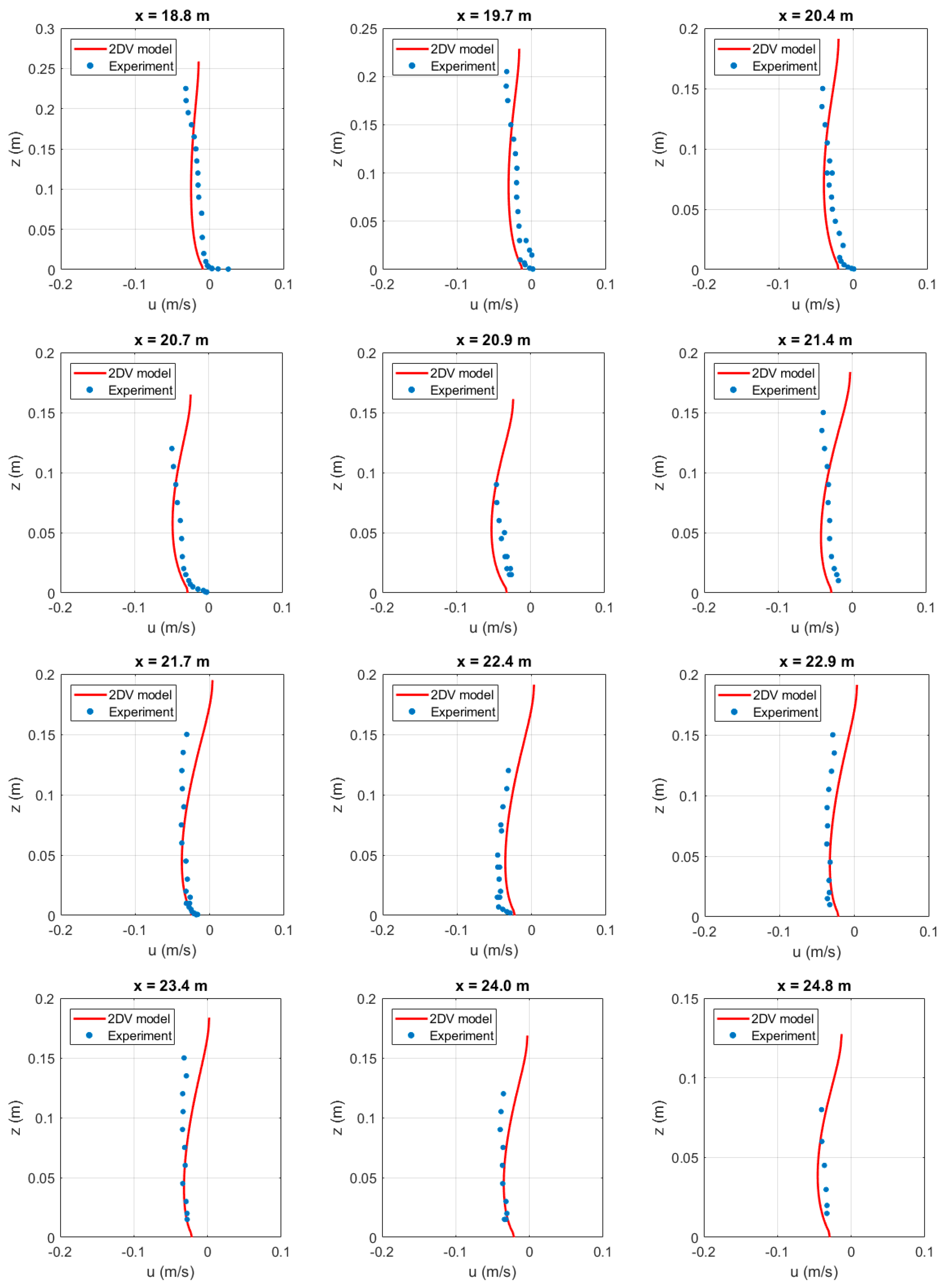
3.6. Breaking Waves Propagating in a Large-Scale Facility

3.6.1. Laboratory Setup and Boundary Conditions

(a) Laboratory setup:

In this section, the 2DV model was employed to simulate the cross-shore and the longshore currents with the input data obtained from the large-scale sediment transport facility (LSTF). The design of the LSTF is presented in detail in the paper of Hamilton and Ebersole [44]. The facility has dimensions of approximately 30 m cross-shore by 50 m longshore by 1.4 m deep. The concrete beach has a longshore dimension of 31 m and a cross-shore dimension of 21 m, with a slope of 1:30. Unidirectional long-crested waves were generated with four piston-type wave generators. An active pumping and recirculation system comprised of 20 independent pumps and pipelines were used to control the cross-shore distribution of mean longshore current. Pumping rates were adjusted iteratively to converge toward the proper setting, based on the measurements along the beach.

The wave conditions at the offshore boundary are given in

Table 5. Incident wave properties at the boundary.

Wave Type	Tp (s)	Hs (m)	$\mathit{\theta }\left({}_{}^0\right)$	h (m)
Irregular	2.5	0.225	10	0.667

. The TMA spectrum (self-similar spectral shape) with the width parameter of 3.3 was employed. It is an extension of deep water spectrum JONSWAP for applications in shallow water.

(b) Surface and bottom boundary conditions:

At the mean water surface, the total shear stress is assumed to vanish, i.e.,

$${\left[\left({\upsilon }_v+K_{fr}+K_b\right)\frac{\partial \overline{u}}{\partial z}\right]}_{z={\overline{\mathsf{\zeta }}}^L}=0,$$

(79)

$${\left[\left({\upsilon }_v+K_{fr}+K_b\right)\frac{\partial \overline{v}}{\partial z}\right]}_{z={\overline{\mathsf{\zeta }}}^L}=0,$$

(80)

where, ${\upsilon }_v={\upsilon }_{mol}+{\upsilon }_v^T$.

The bottom boundary condition in the cross-shore direction is given by:

$${\left[\left({\upsilon }_v+K_{fr}+K_b\right)\frac{\partial \overline{u}}{\partial z}\right]}_{z=-h+\mathsf{\delta }}=-\frac{k_1{D}_f}{\mathsf{\rho }\sigma }-\frac{{\overline{\tau }}_{cw,x}}{\mathsf{\rho }},$$

(81)

According to Longuet-Higgins [4], the bed shear stress in the longshore direction can be calculated based on the local rate of energy dissipation. Therefore:

$${\overline{\tau }}_{cw,y}=-\frac{k_2\left[\left(1-{\alpha }_r\right)D_w+D_r+D_f\right]}{\sigma },$$

(82)

From Equations (52) and (82) the bottom boundary condition in the longshore direction is given by:

$${\overline{v}}_b=\frac{2k_2\left[\left(1-{\alpha }_r\right)D_w+D_r+D_f\right]}{\mathsf{\rho }\sigma f_{cw}\sqrt{{(1.16s)}^2+{\left|{\overline{u}}_b\right|}^2}},$$

(83)

(c) Lateral boundary conditions:

At the offshore, boundary conditions for quasi-Eulerian mean water level and quasi-Eulerian mean velocity components are:

$$\overline{\mathsf{\zeta }}=-\frac{k{a}^2}{2\sinh 2kD},$$

(84)

$$\overline{u}=-\frac{1}{h+{\overline{\mathsf{\zeta }}}^L}{\displaystyle {\int }_{-h+\mathsf{\delta }}^{{\overline{\mathsf{\zeta }}}^L}{\overline{u}}^{S}dz},$$

(85)

$$\overline{v}=\overline{u}\tan \theta ,$$

(86)

At the land boundary, the GLM velocity in the x-direction is zero. Besides, the no-slip boundary condition is assumed for quasi-Eulerian velocity in the y-direction. Then:

$$\overline{u}(z)=-{\overline{u}}^S(z),$$

(87)

$$\overline{v}(z)=0,$$

(88)

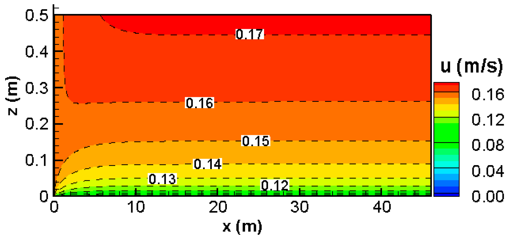
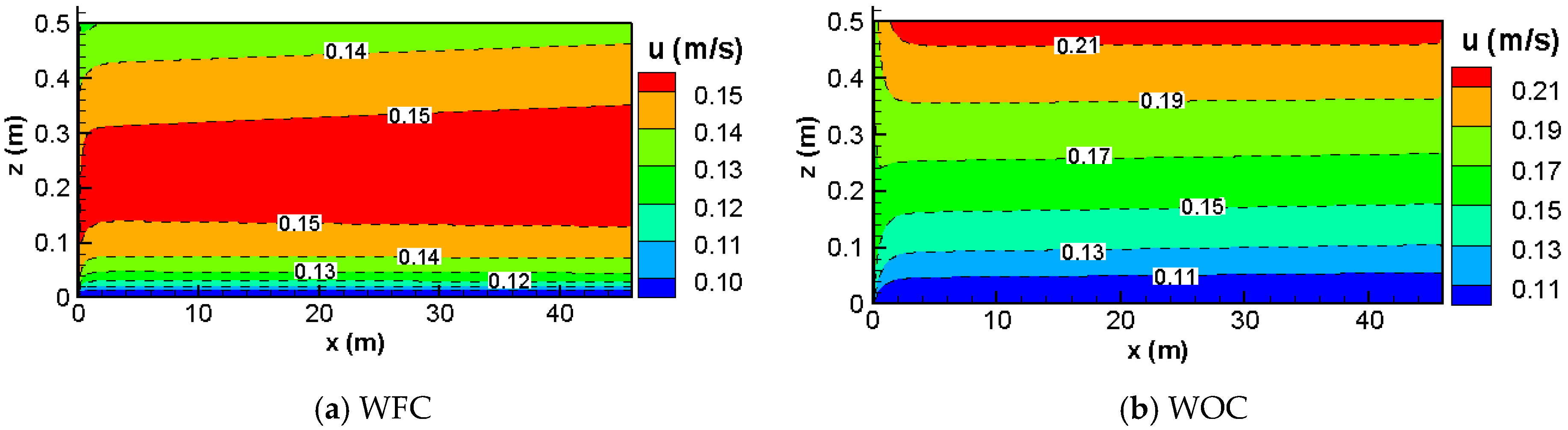
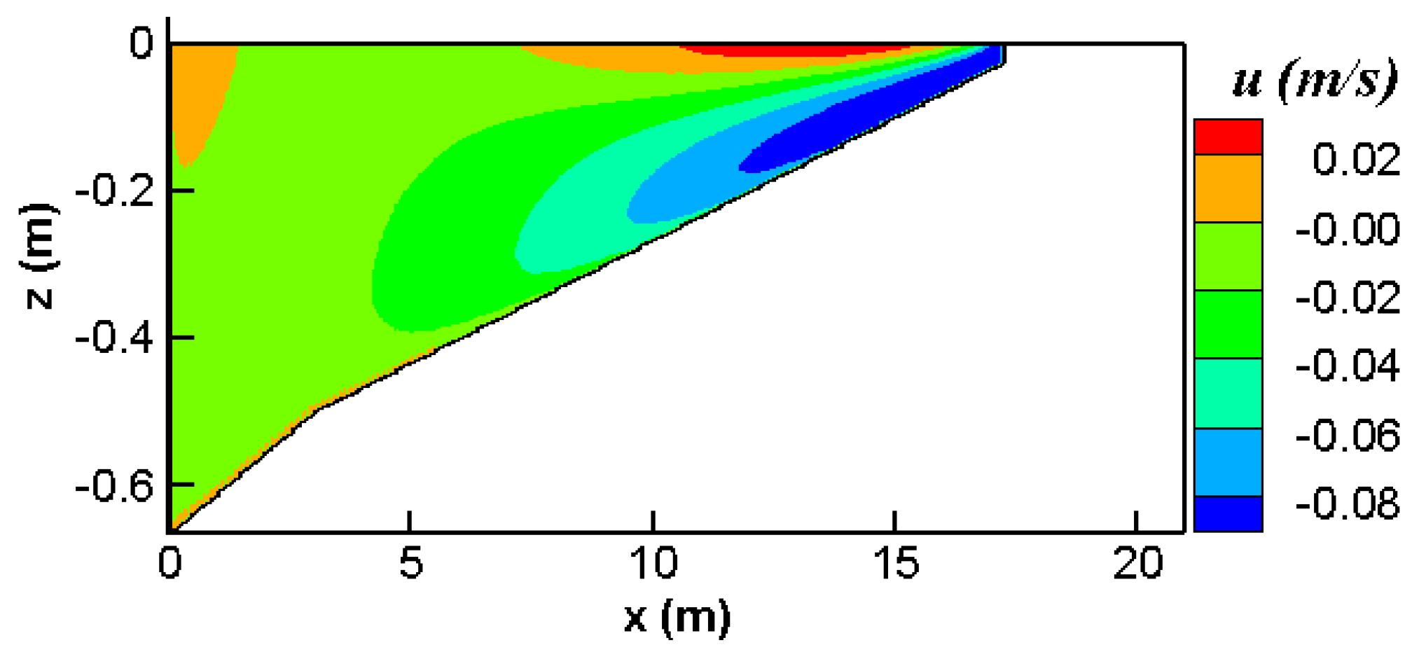
3.6.2. Numerical Results and Discussion

Figure 27 shows the comparison of significant wave height between experimental data and numerical results calculated by the 2DV model. The comparison shows a very good agreement between experimental data and model results.

In Figure 28, a comparison of the mean water level between experimental data and the 2DV model result is given. There was a small difference of about a few millimeters outside the breaking zone. The difference between these two kinds of data was bigger in the area closer to the coastline. It might be due to the recirculation system of the facility or because the experimental data was for a closed basin, so the volume of water in the setup was taken from offshore.

(a) Cross-shore direction:

Figure 29 presents the vertical distribution of wave forcing term $F_{w,1}/\mathsf{\rho }$ and total mixing $F_{tot,1}/\mathsf{\rho }$ at the location $x=10.9 \mathrm{m}$. It shows that momentum caused by wave forcing was completely compensated by total mixing. The total of these two forcing terms was depth-uniform.

Figure 30 shows an overview of the spatial distribution of cross-shore velocity calculated by the 2DV model. It shows that outside the wave breaking zone, the vertical distribution of the quasi-Eulerian mean velocity was almost uniform. However, inside the wave breaking zone, the mean velocity shows a strong vertical shear.

The LSTF data was also employed by Teles, Pires-Silva [45] to validate the TELEMAC 3D model. In Figure 31, comparisons of cross-shore mean velocities between experimental data, results of the TELEMAC 3D model, and results of the 2DV model were carried out at six cross-shore locations.

The results obtained from the 2DV model fit quite well with the experimental data, and much better than the results obtained by the TELEMAC 3D model in most of the cross-sections. Closer to the surface and the land boundary the difference between experimental data and 2DV model results became bigger. The difference might be due to the use of empirical formulas for the wave-induced forcing, and the return flow in the facility. Improvement of these formulas making use of the large body of literature on the return flow profiles is recommendable but outside the scope of this study.

(b) Longshore direction:

Figure 32 shows the vertical distribution of the wave-induced forcing $F_{w,2}/\mathsf{\rho }$ and total mixing $F_{tot,2}/\mathsf{\rho }$ in the longshore direction at $x=10.9 \mathrm{m}$. It shows that the total mixing $F_{tot,2}$ is balanced by wave-induced forcing $F_{tot,2}$. The total forcing $\left(F_{w,2}+F_{tot,2}\right)$ is depth-uniform.

The cross-shore distribution of the longshore velocity calculated by the 2DV numerical model is presented in Figure 33. According to the results, the longshore velocity increases shoreward. The maximum magnitude of the longshore velocity reached approximately 0.35 m/s at the position $x\approx 14$ m. After this point, the longshore velocity was decreased toward the shoreline.

In Figure 34, a comparison between experimental data and numerical results at one-third of the water depth above the bottom is given. It shows that the results obtained by the 2DV model agreed well with the experimental data and matched the observed cross-shore distribution better than the results obtained by the TELEMAC 3D model.

The comparison of the longshore velocities at different vertical cross-sections is given in Figure 35. The results of the TELEMAC 3D model show quite good agreement at four locations from x = 9.5 m to x = 13.9 m. However, at the location near the offshore x = 7.1 m and the location near the coastline x = 15.3 m the differences between experimental data and results from the TELEMAC 3D model were significant. In contrast, the results of the 2DV model show good agreement with experimental data at all six cross-sections.

4. Discussion

Following Van Rijn [35], the bottom boundary layer thickness $\mathsf{\delta }$ was calculated by the Formula (61). In this, the effect of mean current on bottom boundary layer thickness was neglected. However, interactions of current with wave boundary layer and waves with current boundary layer led to the enhancement of current-induced friction, wave energy dissipation, and bed shear stress. Then, both waves and current should be considered in calculating bottom boundary thickness. In this paper, the formula given by Van Rijn [35] was modified to take into account the effect of ambient current. The use of the modified formula obtained a better agreement with experimental data than the use of the original formula of Van Rijn [35].

In the work of Nielsen and You [32], an empirical coefficient $C_{WR}$ was proposed to account for the effect of strong ambient current on the vertical distribution of wave radiation stress components. However, that coefficient is only applied to regular waves. In this work, a modified formula was proposed to apply for random waves. With that modification, the mean current profiles calculated by the 2DV model agreed well with experimental data obtained by Klopman [41].

In breaking wave conditions, dissipative wave forcing terms were estimated by using empirical formulas introduced by Uchiyama, McWilliams [14]. The cross-shore velocity profiles obtained by the 2DV model showed good agreement with experimental data presented in the works of Boers [43] and Hamilton and Ebersole [44]. However, there are differences between model results and observed data near the breaking points. It requires further research on the vertical distribution of wave breaking induced forcing. In the longshore direction, the effect of breaking wave-induced forcing was small. Then, the longshore current data calculated by the 2DV model fitted very well with experimental data.

The LSTF test was also employed by Teles, Pires-Silva [45] to validate the TELEMAC 3D model. That model was developed based on the work of Ardhuin, Rascle [19], and Bennis, Ardhuin [39]. As indicated by Ardhuin, Rascle [19], their equations are only expected to give qualitative results for surf zone applications. The comparison presented in the previous part also showed that the 2DV model obtained a better agreement with observed data than TELEMAC 3D model.

5. Conclusions

In this paper, a new set of equations of motion written in terms of quasi-Eulerian mean velocity was developed based on the GLM method. The new equations were valid from the bottom to the mean water surface even in the presence of finite-amplitude waves. These equations are practical for a wide range of applications from deep water to shallow water areas. All terms in the equations are expressed to the second-order of the wave amplitude. Both non-wave forcing and wave-induced forcing terms are under consideration. When the wave height is infinitesimal, the quasi-Eulerian mean equations of motion reduce to the classical Eulerian mean equations of motion. In cases of density stratification, the buoyancy effect should be included as external forcing.

In the work of Longuet-Higgins and Stewart [2], the effects of waves on the mean current are expressed in terms of the traditional radiation stress concept. It is a depth-integrated term and is only suitable for the depth-averaged equations of motion. In 3D problems, that concept is no longer suitable. In this paper, a depth-dependent wave radiation stress concept was introduced. Then, the effects of surface waves on the mean current could be specified at any level of the water column. The vertical distribution of the mean current was described in detail with the use of a depth-dependent wave radiation stress tensor. With the use of an empirical coefficient $C_{WR}$, the depth-dependent radiation stress could be calculated in the condition of a strong ambient current. It is noticed that the vertical integration of the new depth-dependent wave radiation stress coincided with the traditional radiation stress.

A 2DV numerical model was developed to validate the new quasi-Eulerian mean equations of motion. The turbulent viscosity and wave-induced mixing were calculated by a simple submodel with the assumption of constant-parabolic distribution. The model shows a better comparison with experimental data than previous studies. The model passed the well-known adiabatic condition suggested by Ardhuin, Rascle [19]. It does not produce spurious velocities when the waves propagate on a sloping bottom. As a result, vertical uniform distribution of quasi-Eulerian mean horizontal velocity was obtained even on the slope.

Subsequently, the experiment of Klopman [41] for random waves was employed to validate the 2DV model in the condition of non-breaking waves combined with a current. The comparison between experimental data and numerical results showed very good agreement in the whole vertical section even in areas that were very close to the bed. In the condition of breaking waves, two experiments presented in the dissertation of Boers [43] were used. It was shown that the new equations performed very well for the experiment of smaller wave height (test 1C). In the experiment of bigger wave height (test 1B), the vertical distribution of the mean velocity near the breaking point gave qualitatively correct results. In the comparison of longshore current in the LSTF test [44], a good agreement was found not only for depth-averaged longshore current but also for depth varying longshore current. For cross-shore currents, there was a difference between model results and experimental data in the wave breaking zone. The difference between the experimental data and model results in tests 1B and LSTF was likely to be due to the empirical formulas for wave breaking that were strong simplifications of the complex breaking process. Further tuning of such formulations against a large number of datasets on wave decay and generated longshore and cross-shore currents was recommended.

Finally, with the use of quasi-Eulerian mean variables, the new set of equations of motion can be easily implemented to existing 3D models developed based on the classical Eulerian mean method. The implementation is straightforward and does not require much effort. It can improve significantly the results of simulating coastal processes such as coastal sediment transport, transport of plastic, and other pollutants such as oil slicks.

References

1. Longuet-Higgins, M.S.; Stewart, R.W. Changes in the form of short gravity waves on long waves and tidal currents. J. Fluid Mech. 1960, 8, 565–583. [Google Scholar] [CrossRef]
2. Longuet-Higgins, M.S.; Stewart, R. Radiation stress and mass transport in gravity waves, with application to ‘surf beats’. J. Fluid Mech. 1962, 13, 481–504. [Google Scholar] [CrossRef]
3. Longuet-Higgins, M.S.; Stewart, R. Radiation Stresses in Water Waves; A Physical Discussion, with Applications. In Deep Sea Research and Oceanographic Abstracts; Elsevier: Amsterdam, The Netherlands, 1964; pp. 529–562. Available online: https://0-www-sciencedirect-com.brum.beds.ac.uk/science/article/abs/pii/0011747164900014 (accessed on 10 January 2021).
4. Longuet-Higgins, M.S. Longshore currents generated by obliquely incident sea waves: 1. J. Geophys. Res. 1970, 75, 6778–6789. [Google Scholar] [CrossRef]
5. Bowen, A.J. The generation of longshore currents on a plane beach. J. Mar. Res. 1969, 27, 206–215. [Google Scholar]
6. Thornton, E.B. Variation of longshore current across the suft zone. Coast. Eng. Proc. 1970, 1, 18. [Google Scholar] [CrossRef] [Green Version]
7. Xie, L.; Wu, K.; Pietrafesa, L.; Zhang, C. A numerical study of wave-current interaction through surface and bottom stresses: Wind-driven circulation in the South Atlantic Bight under uniform winds. J. Geophys. Res. Oceans (1978–2012) 2001, 106, 16841–16855. [Google Scholar] [CrossRef] [Green Version]
8. Xia, H.; Xia, Z.; Zhu, L. Vertical variation in radiation stress and wave-induced current. Coast. Eng. 2004, 51, 309–321. [Google Scholar] [CrossRef]
9. Craik, A.; Leibovich, S. A rational model for Langmuir circulations. J. Fluid Mech. 1976, 73, 401–426. [Google Scholar] [CrossRef] [Green Version]
10. Leibovich, S. On the evolution of the system of wind drift currents and Langmuir circulations in the ocean. Part 1. Theory and averaged current. J. Fluid Mech. 1977, 79, 715–743. [Google Scholar] [CrossRef]
11. McWilliams, J.C.; Restrepo, J.M. The wave-driven ocean circulation. J. Phys. Oceanogr. 1999, 29, 2523–2540. [Google Scholar] [CrossRef]
12. McWilliams, J.C.; Restrepo, J.M.; Lane, E.M. An asymptotic theory for the interaction of waves and currents in coastal waters. J. Fluid Mech. 2004, 511, 135–178. [Google Scholar] [CrossRef]
13. Newberger, P.; Allen, J.S. Forcing a three-dimensional, hydrostatic, primitive-equation model for application in the surf zone: 1. Formulation. J. Geophys. Res. Ocean. 2007, 112. [Google Scholar] [CrossRef] [Green Version]
14. Uchiyama, Y.; McWilliams, J.C.; Shchepetkin, A.F. Wave–current interaction in an oceanic circulation model with a vortex-force formalism: Application to the surf zone. Ocean Model. 2010, 34, 16–35. [Google Scholar] [CrossRef]
15. Kumar, N.; Voulgaris, G.; Warner, J.C.; Olabarrieta, M. Implementation of the vortex force formalism in the coupled ocean-atmosphere-wave-sediment transport (COAWST) modeling system for inner shelf and surf zone applications. Ocean Model. 2012, 47, 65–95. [Google Scholar] [CrossRef]
16. Lane, E.M.; Restrepo, J.M.; McWilliams, J.C. Wave–current interaction: A comparison of radiation-stress and vortex-force representations. J. Phys. Oceanogr. 2007, 37, 1122–1141. [Google Scholar] [CrossRef] [Green Version]
17. Mellor, G. The three-dimensional current and surface wave equations. J. Phys. Oceanogr. 2003, 33, 1978–1989. [Google Scholar] [CrossRef]
18. Mellor, G.L. The depth-dependent current and wave interaction equations: A revision. J. Phys. Oceanogr. 2008, 38, 2587–2596. [Google Scholar] [CrossRef]
19. Ardhuin, F.; Rascle, N.; Belibassakis, K.A. Explicit wave-averaged primitive equations using a generalized Lagrangian mean. Ocean Model. 2008, 20, 35–60. [Google Scholar] [CrossRef] [Green Version]
20. Mellor, G. A combined derivation of the integrated and vertically resolved, coupled wave–current equations. J. Phys. Oceanogr. 2015, 45, 1453–1463. [Google Scholar] [CrossRef]
21. Mellor, G. On theories dealing with the interaction of surface waves and ocean circulation. J. Geophys. Res. Ocean. 2016, 121, 4474–4486. [Google Scholar] [CrossRef]
22. Ardhuin, F.; Suzuki, N.; McWilliams, J.C.; Aiki, H. Comments on “A Combined Derivation of the Integrated and Vertically Resolved, Coupled Wave–Current Equations”. J. Phys. Oceanogr. 2017, 47, 2377–2385. [Google Scholar] [CrossRef]
23. Andrews, D.; McIntyre, M. An exact theory of nonlinear waves on a Lagrangian-mean flow. J. Fluid Mech. 1978, 89, 609–646. [Google Scholar] [CrossRef] [Green Version]
24. Leibovich, S. On wave-current interaction theories of Langmuir circulations. J. Fluid Mech. 1980, 99, 715–724. [Google Scholar] [CrossRef] [Green Version]
25. Dingemans, M.W. Water Wave Propagation over Uneven Bottoms: Linear Wave Propagation; World Scientific: Singapore, 1997; Volume 13. [Google Scholar]
26. Groeneweg, J. Wave-Current Interactions in a Generalized Lagrangian Mean Formulation. Ph.D. Thesis, Delft University of Technology, Delft, The Netherland, 1999. [Google Scholar]
27. Walstra, D.; Roelvink, J.; Groeneweg, J. Calculation of wave-driven currents in a 3D mean flow model. In Coastal Engineering 2000; 2001; pp. 1050–1063. Available online: https://ascelibrary.org/doi/abs/10.1061/40549(276)81 (accessed on 13 January 2021).
28. Roelvink, J.; Reniers, A. A Guide to Modeling Coastal Morphology; World Scientific: Singapore, 2011; Volume 12. [Google Scholar]
29. Deigaard, R.; Fredsøe, J. Shear stress distribution in dissipative water waves. Coast. Eng. 1989, 13, 357–378. [Google Scholar] [CrossRef]
30. You, Z.-J. On the vertical distribution of< ũ w ~ > by FJ Rivero and AS Arcilla: Comments. Coast. Eng. 1997, 30, 305–310. [Google Scholar] [CrossRef]
31. Supharatid, S.; Tanaka, H.; Shuto, N. Interactions of waves and current (Part I: Experimental investigation). Coast. Eng. Jpn. 1992, 35, 167–186. [Google Scholar] [CrossRef]
32. Nielsen, P.; You, Z.-J. Eulerian mean velocities under non-breaking waves on horizontal bottoms. In Coastal Engineering 1996; 1997; pp. 4066–4078. Available online: https://ascelibrary.org/doi/abs/10.1061/9780784402429.314 (accessed on 10 January 2021).
33. Ockenden, M.; Soulsby, R. Sediment Transport by Currents Plus Irregular Waves. 1994. Available online: https://eprints.hrwallingford.com/347/ (accessed on 13 January 2021).
34. Soulsby, R. Dynamics of Marine Sands: A Manual for Practical Applications. Thomas Telford, 1997. Available online: https://www.infona.pl/resource/bwmeta1.element.elsevier-69102d77-8480-3ca9-adc0-a09c289eb654 (accessed on 13 January 2021).
35. Van Rijn, L.C. Principles of Fluid Flow and Surface Waves in Rivers, Estuaries, Seas and Oceans; Aqua Publications: Amsterdam, The Netherlands, 2011; Available online: https://www.aquapublications.nl/Contentsbook1.pdf (accessed on 13 January 2021).
36. Feddersen, F.; Guza, R.; Elgar, S.; Herbers, T. Velocity moments in alongshore bottom stress parameterizations. J. Geophys. Res. Ocean. 2000, 105, 8673–8686. [Google Scholar] [CrossRef]
37. Longuet-Higgins, M. The mechanics of the surf zone. In Theoretical and Applied Mechanics; Springer: Berlin/Heidelberg, Germany, 1973; pp. 213–228. [Google Scholar] [CrossRef]
38. Stelling, G.S.; Busnelli, M.M. Numerical simulation of the vertical structure of discontinuous flows. Int. J. Numer. Methods Fluids 2001, 37, 23–43. [Google Scholar] [CrossRef]
39. Bennis, A.-C.; Ardhuin, F.; Dumas, F. On the coupling of wave and three-dimensional circulation models: Choice of theoretical framework, practical implementation and adiabatic tests. Ocean Model. 2011, 40, 260–272. [Google Scholar] [CrossRef] [Green Version]
40. Belibassakis, K.; Athanassoulis, G. Extension of second-order Stokes theory to variable bathymetry. J. Fluid Mech. 2002, 464, 35–80. [Google Scholar] [CrossRef] [Green Version]
41. Klopman, G. Vertical Structure of the Flow Due to Waves and Currents: Laser-Doppler Flow Measurements for Waves following or Opposing a Current. Delft Hydraulics, Report No. H840.32, Part 2. 1994. Available online: https://repository.tudelft.nl/islandora/object/uuid:181f5c9c-f66f-4103-abe6-c4633137e351 (accessed on 10 January 2021).
42. Fredsøe, J.; Deigaard, R. Mechanics of Coastal Sediment Transport; World Scientific: Singapore, 1992; Volume 3. [Google Scholar]
43. Boers, M. Surf Zone Turbulence. 2005. Available online: https://repository.tudelft.nl/islandora/object/uuid:71428ad5-0658-49f7-b83e-0deb26b668cf (accessed on 10 January 2021).
44. Hamilton, D.G.; Ebersole, B.A. Establishing uniform longshore currents in a large-scale sediment transport facility. Coast. Eng. 2001, 42, 199–218. [Google Scholar] [CrossRef]
45. Teles, M.J.; Pires-Silva, A.A.; Benoit, M. Three dimensional modelling of wave-current interactions in the coastal zone with a fully coupled system. Geography. 2013. Available online: https://www.researchgate.net/profile/Maria_Teles2/publication/315066486_THREE_DIMENSIONAL_MODELLING_OF_WAVE-CURRENT_INTERACTIONS_IN_THE_COASTAL_ZONE_WITH_A_FULLY_COUPLED_SYSTEM/links/58c9539f4585157512329679/THREE-DIMENSIONAL-MODELLING-OF-WAVE-CURRENT-INTERACTIONS-IN-THE-COASTAL-ZONE-WITH-A-FULLY-COUPLED-SYSTEM.pdf (accessed on 10 January 2021).
Figure 1. A flowchart describing the methodology of the research.
Jmse 09 00076 g001
Figure 2. Bathymetry of the computational area.
Jmse 09 00076 g002
Figure 3. Spatial distribution of Stokes drift.
Jmse 09 00076 g003
Figure 4. Distribution of mean water level ζ ¯ .
Jmse 09 00076 g004
Figure 5. Distribution of F w , 1 / ρ ( m / s 2 ).
Jmse 09 00076 g005
Figure 6. Vertical distribution of the generalized Lagrangian mean (GLM) velocity and quasi-Eulerian mean velocity.
Jmse 09 00076 g006
Figure 7. Vertical distribution of the Eulerian-mean velocity.
Jmse 09 00076 g007
Figure 8. Vertical distribution of Reynolds shear stress u t w t ¯ in the CO condition.
Jmse 09 00076 g008
Figure 9. Vertical distribution of turbulent viscosity ( υ v T ).
Jmse 09 00076 g009
Figure 10. Vertical distribution of the wave radiation stress component u ˜ w ˜ ¯ C S .
Jmse 09 00076 g010
Figure 11. Vertical distribution of wave-induced forcing terms.
Jmse 09 00076 g011
Figure 12. Reynolds turbulent stress u t w t ¯ in the CO condition.
Jmse 09 00076 g012
Figure 13. Spatial distribution of quasi-Eulerian mean velocity in the CO condition.
Jmse 09 00076 g013
Figure 14. Vertical distribution of quasi-Eulerian mean velocity in the CO condition.
Jmse 09 00076 g014
Figure 15. Spatial distribution of mean velocity fields in the WO condition.
Jmse 09 00076 g015
Figure 16. Vertical distribution of quasi-Eulerian mean velocity in the WO condition.
Jmse 09 00076 g016
Figure 17. Spatial distribution of quasi-Eulerian mean velocity.
Jmse 09 00076 g017
Figure 18. Vertical distribution of quasi-Eulerian mean velocity in the linear scale.
Jmse 09 00076 g018
Figure 19. Vertical distribution of quasi-Eulerian mean velocity in the semilogarithmic scale.
Jmse 09 00076 g019
Figure 20. The bottom profile.
Jmse 09 00076 g020
Figure 21. Distribution of significant wave height H S .
Jmse 09 00076 g021
Figure 22. Distribution of wave-induced forcing terms at x = 22.9   m .
Jmse 09 00076 g022
Figure 23. Distribution of mean water level ζ ¯ .
Jmse 09 00076 g023
Figure 24. Distribution of Stokes drift (a,b) and quasi-Eulerian mean velocity (c,d).
Jmse 09 00076 g024aJmse 09 00076 g024b
Figure 25. Vertical distribution of horizontal mean velocity in test 1B.
Jmse 09 00076 g025aJmse 09 00076 g025b
Figure 26. Vertical distribution of horizontal mean velocity in test 1C.
Jmse 09 00076 g026aJmse 09 00076 g026bJmse 09 00076 g026c
Figure 27. Distribution of significant wave height H S .
Jmse 09 00076 g027
Figure 28. Distribution of the mean water level ζ ¯ .
Jmse 09 00076 g028
Figure 29. Vertical distribution of wave-induced forcing terms.
Jmse 09 00076 g029
Figure 30. Distribution of cross-shore velocity.
Jmse 09 00076 g030
Figure 31. Vertical profiles of cross-shore velocity.
Jmse 09 00076 g031
Figure 32. Vertical distribution of wave-induced forcing terms.
Jmse 09 00076 g032
Figure 33. Distribution of the longshore velocity.
Jmse 09 00076 g033
Figure 34. Longshore velocity at z = 2 h / 3 .
Jmse 09 00076 g034
Figure 35. Vertical profiles of the longshore velocity at different locations.
Jmse 09 00076 g035aJmse 09 00076 g035b